Lower Runtime Bounds for Integer Programs
?F. Frohn1, M. Naaf1, J. Hensel1, M. Brockschmidt2, and J. Giesl1
1 LuFG Informatik 2, RWTH Aachen University, Germany
2 Microsoft Research, Cambridge, UK
Abstract. We present a technique to inferlower bounds on the worst- case runtime complexity of integer programs. To this end, we construct symbolic representations of program executions using a framework for ite- rative, under-approximating program simplification. The core of this sim- plification is a method for (under-approximating) program acceleration based on recurrence solving and a variation of ranking functions. After- wards, we deduce asymptotic lower bounds from the resulting simpli- fied programs. We implemented our technique in our toolLoATand show that it infers non-trivial lower bounds for a large number of examples.
1 Introduction
Recent advances in program analysis yield efficient methods to findupper bounds on the complexity of sequential integer programs. Here, one usually considers
“worst-case complexity”, i.e., for any variable valuation, one analyzes the length of the longest execution starting from that valuation. But in many cases, in addition to upper bounds, it is also important to find lower bounds for this notion of complexity. Together with an analysis for upper bounds, this can be used to infer tight complexity bounds. Lower bounds also have important applications in secu- rity analysis, e.g., to detect possible denial-of-service or side-channel attacks, as programs whose runtime depends on a secret parameter “leak” information about that parameter. In general,concretelower bounds that hold for arbitrary variable valuations can hardly be expressed concisely. In contrast,asymptotic bounds are easily understood by humans and witness possible attacks in a convenient way.
We first introduce our program model in Sect. 2. In Sect. 3, we show how to use a variation of classical ranking functions which we call metering func- tions to under-estimate the number of iterations of a simple loop (i.e., a single transitiontlooping on a location`). Then, we present a framework for repeated program simplifications in Sect. 4. It simplifies full programs (with branching and sequences of possibly nested loops) to programs with only simple loops. More- over, it eliminates simple loops by (under-)approximating their effect using a combination of metering functions and recurrence solving. In this way, programs are transformed tosimplified programs without loops. In Sect. 5, we then show how to extract asymptotic lower bounds and variables that influence the runtime from simplified programs. Finally, we conclude with an experimental evaluation of our implementationLoAT in Sect. 6. For all proofs, we refer to [16].
?Supported by the DFG grant GI 274/6-1 and the Air Force Research Laboratory (AFRL).
Related Work While there are many techniques to infer upper bounds on the worst-case complexity of integer programs (e.g., [1–4, 8, 9, 14, 19, 26]), there is little work onlower bounds. In [3], it is briefly mentioned that their technique could also be adapted to infer lower instead of upper bounds for abstract cost rules, i.e., integer procedures with (possibly multiple) outputs. However, this only considers best-case lower bounds instead of worst-case lower bounds as in our technique. Upper and lower bounds forcost relations are inferred in [1]. Cost relations extend recurrence equations such that, e.g., non-determinism can be modeled. However, this technique also considers best-case lower bounds only.
A method for best-case lower bounds for logic programs is presented in [11].
Moreover, we recently introduced a technique to infer worst-case lower bounds for term rewrite systems (TRSs) [15]. However, TRSs differ fundamentally from the programs considered here, since they do not allow integers and have no notion of a “program start”. Thus, the technique of [15], based on synthesizing families of reductions by automatic induction proofs, is very different to the present paper.
To simplify programs, we use a variant ofloop acceleration to summarize the effect of applying a loop repeatedly. Acceleration is mostly used in over- approximating settings (e.g., [13, 17, 21, 24]), where handling non-determinism is challenging, as loop summaries have to coverall possible non-deterministic choi- ces. However, our technique is under-approximating, i.e., we can instantiate non- deterministic values arbitrarily. In contrast to the under-approximating acceler- ation technique in [22], instead of quantifier elimination we use an adaptation of ranking functions to under-estimate the number of loop iterations symbolically.
2 Preliminaries
We consider sequential non-recursive imperative integer programs, allowing non- linear arithmetic and non-determinism, whereas heap usage and concurrency are not supported. While most existing abstractions that transform heap pro- grams to integer programs are “over-approximations”, we would need an under- approximating abstraction to ensure that the inference of worst-case lower bounds is sound. As in most related work, we treat numbers as mathematical integersZ. However, the transformation from [12] can be used to handle machine integers correctly by inserting explicit normalization steps at possible overflows.
A(V) is the set of arithmetic terms3 over the variables V and F(V) is the set of conjunctions4of (in)equations over A(V). So forx, y∈ V, A(V) contains terms likex·y+ 2y andF(V) contains formulas such asx·y≤2y∧y >0.
3 Our implementation only supports addition, subtraction, multiplication, division, and exponentiation. Since we consider integer programs, we only allow programs where all variable values are integers (so in contrast tox= 12x, the assignmentx= 12x+12x2is permitted). While our program simplification technique preserves this property, we do not allow division or exponentiation in theinitial program to ensure its validity.
4 Note that negations can be expressed by negating (in)equations directly, and disjunc- tions in programs can be expressed using multiple transitions.
`0:y= 0
`1:whilex >0do y=y+x x=x−1 done z=y
`2:whilez >0do u=z−1
`3: whileu >0do u=u−random(0, ω) done
z=z−1 done
`0
`1
`2
`3
t0[1]:y0= 0 t1[1]:if(x >0)
y0=y+x
x0=x−1 t2[1]:if(x≤0) z0=y t3[1]:if(z >0)
u0=z−1 t4[1]:if
u >0∧ tv>0
u0=u−tv t5[1]:if(u≤0) z0=z−1
Fig. 1: Example integer program
We fix a finite set ofprogram variables PVand represent integer programs as directed graphs. Nodes are programlocationsLand edges are programtransitions T whereL contains a canonical start location `0. W.l.o.g., no transition leads back to`0and all transitionsT are reachable from`0. To model non-deterministic program data, we introduce pairwise disjoint finite sets of temporary variables T V` withPV ∩ T V`=∅and define V`=PV ∪ T V` for all locations `∈ L.
Definition 1 (Programs).Configurations (`,v)consist of a location`∈ Land a valuation v : V` → Z. Val` =V` → Z is the set of all valuations for ` ∈ L and valuations are lifted to termsA(V`)and formulas F(V`)as usual. Atransi- tiont= (`, γ, η, c, `0)can evaluate a configuration(`,v)if theguardγ∈ F(V`)is satisfied (i.e., v(γ) holds) to a new configuration(`0,v0). The updateη:PV → A(V`)maps any x∈ PV to a term η(x)where v(η(x))∈Z for all v∈ Val`. It determinesv0 by settingv0(x) =v(η(x))forx∈ PV, whilev0(x)forx∈ T V`0 is arbitrary. Such an evaluation step has costk=v(c)forc∈ A(V`)and is writ- ten(`,v)→t,k (`0,v0). We usesrc(t) =`,guard(t) =γ,cost(t) =c, anddest(t) =
`0. We sometimes drop the indicest, k and write (`,v)→∗k (`0,v0)if (`,v)→k1
· · · →km (`0,v0)andP
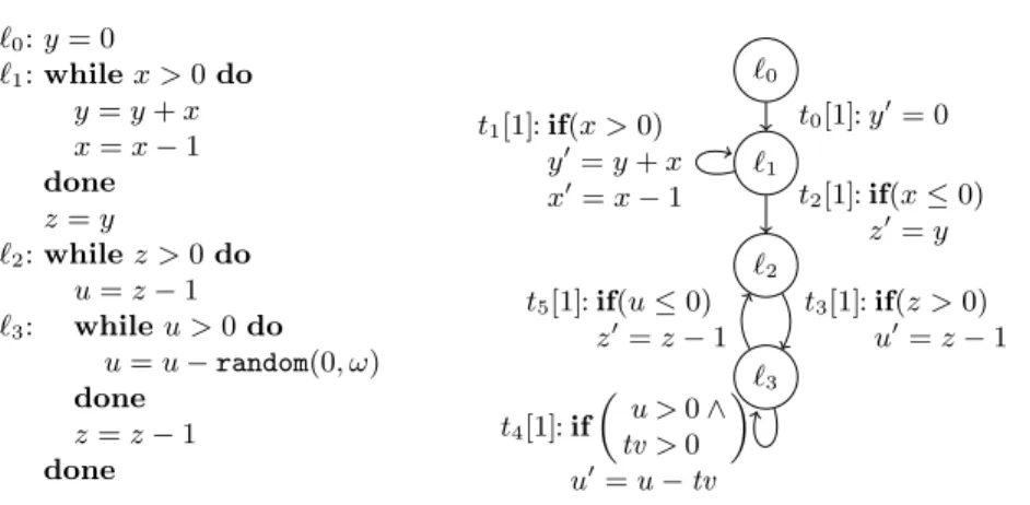
1≤i≤mki =k. Aprogramis a set of transitionsT. Fig. 1 shows an example, where the pseudo-code on the left corresponds to the program on the right. Here,random(x, y) returns a random integermwith x <
m < yand we fix−ω < m < ωfor all numbersm. The loop at location`1setsyto a value that is quadratic inx. Thus, the loop at`2is executed quadratically often where in each iteration, the inner loop at`3 may also be repeated quadratically often. Thus, the length of the program’s worst-case execution is a polynomial of degree 4 in x. Our technique can infer such lower bounds automatically.
In the graph of Fig. 1, we write the costs of a transition in [ ] next to its name and represent the updates by imperative commands. We usexto refer to the value of the variable xbefore the update andx0 to refer to x’s value after the update. Here,PV={x, y, z, u},T V`3 ={tv}, andT V`=∅for all locations
`6=`3. We have (`3,v)→t4(`3,v0) for all valuationsvwherev(u)>0,v(tv)>0, v0(u) =v(u)−v(tv), andv0(v) =v(v) for all v∈ {x, y, z}.
Our goal is to find a lower bound on the worst-case runtime of a programT. To this end, we define its derivation height [18] by a function dhT that operates on valuations v of the program variables (i.e.,v is not defined for temporary variables). The functiondhT mapsvto the maximum of the costs of all evaluation sequences starting in configurations (`0,v`0) wherev`0 is an extension of v to V`0. So in our example we havedhT(v) = 2 for all valuationsv wherev(x) = 0, since then we can only apply the transitionst0 andt2once. For all valuations v withv(x)>1, our method will detect that the worst-case runtime of our program is at least 18v(x)4+14v(x)3+78v(x)2+74v(x). From this concrete lower bound, our approach will infer that the asymptotic runtime of the program is inΩ(x4).
In particular, the runtime of the program depends onx. Hence, ifxis “secret”, then the program is vulnerable to side-channel attacks.
Definition 2 (Derivation Height).LetVal =PV →Z. Thederivation height dhT : Val → R≥0∪ {ω} of a program T is defined as dhT(v) = sup{k ∈ R |
∃v`0 ∈ Val`0, `∈ L,v`∈ Val`. v`0|PV =v ∧ (`0,v`0)→∗k (`,v`)}.
Since →∗k also permits evaluations with 0 steps, we always have dhT(v) ≥ 0.
Obviously,dhT is not computable in general, and thus our goal is to compute a lower bound that is as precise as possible (i.e., a lower bound which is, e.g., unbounded,5exponential, or a polynomial of a degree as high as possible).
3 Estimating the Number of Iterations of Simple Loops
We now show how to under-estimate the number of possible iterations of asimple loopt= (`, γ, η, c, `). More precisely, we infer a termb∈ A(V`) such that for allv
∈ Val` with v |=γ, there is av0 ∈ Val` with (`,v)→dv(b)et (`,v0). Here,dke= min{m ∈ N | m ≥ k} for all k ∈ R. Moreover, (`,v) →mt (`,v0) means that (`,v) = (`,v0)→t,k1 (`,v1)→t,k2 · · · →t,km (`,vm) = (`,v0) for some costsk1, . . . , km. We say that (`,v)→mt (`,v0)preservesT V` iffv(tv) =vi(tv) =v0(tv) for all tv ∈ T V` and all 0≤i ≤m. Accordingly, we lift the update η to arbi- trary arithmetic terms by leaving temporary variables unchanged (i.e., ifPV= {x1, . . . , xn}and b∈ A(V`), thenη(b) =b[x1/η(x1), . . . , xn/η(xn)], where [x/a]
denotes the substitution that replaces all occurrences of the variablexbya).
To find such estimations, we use an adaptation of ranking functions [2, 6, 25]
which we callmetering functions. We say that a term b ∈ A(V`) is a ranking function6fort= (`, γ, η, c, `) iff the following conditions hold.
γ =⇒ b >0 (1) γ =⇒ η(b)≤b−1 (2)
So e.g.,xis a ranking function fort1in Fig. 1. IfT V`=∅, then for any valuation v∈ Val,v(b)over-estimates the number of repetitions of the loopt: (2) ensures thatv(b) decreases at least by 1 in each loop iteration, and (1) requires thatv(b) is positive whenever the loop can be executed. In contrast, metering functions areunder-estimations for the maximal number of repetitions of a simple loop.
5 Programs withdhT(v) =ωresult from non-termination or non-determinism. As an example, consider the programx=random(0, ω);whilex >0dox=x−1done.
6 In the following, we often use arithmetic termsA(V`) to denote functionsV`→R.
Definition 3 (Metering Function). Lett= (`, γ, η, c, `) be a transition. We callb∈ A(V`)a metering functionfort iff the following conditions hold:
¬γ =⇒ b≤0 (3) γ =⇒ η(b)≥b−1 (4) Here, (4) ensures thatv(b) decreases at most by 1 in each loop iteration, and (3) requires thatv(b) is non-positive if the loop cannot be executed. Thus, the
loop can be executed at least v(b) times (i.e.,v(b) is an under-estimation).
For the transition t1 in the example of Fig. 1, x is also a valid metering function. Condition (3) requires¬x >0 =⇒ x≤0 and (4) requires x >0 =⇒ x−1≥x−1. While xis a meteringand a ranking function, x2 is a metering, but not a ranking function fort1. Similarly,x2 is a ranking, but not a metering function fort1. Thm. 4 states that a simple loop t with a metering functionb can be executed at leastdv(b)etimes when starting with the valuationv.
Theorem 4 (Metering Functions are Under-Estimations). Letbbe a me- tering function fort= (`, γ, η, c, `). Thenbunder-estimatest, i.e., for allv∈ Val`
with v|=γ there is an evaluation (`,v)→dv(b)et (`,v0)that preservesT V`. Our implementation builds upon a well-known transformation based on Farkas’ Lemma [6, 25] to find linear metering functions. The basic idea is to search for coefficients of a linear template polynomial b such that (3) and (4) hold for all possible instantiations of the variablesV`. In addition to (3) and (4), we also require (1) to avoid trivial solutions likeb= 0. Here, the coefficients ofb are existentially quantified, while the variables fromV`are universally quantified.
As in [6, 25], eliminating the universal quantifiers using Farkas’ Lemma allows us to use standard SMT solvers to search forb’s coefficients efficiently.
When searching for a metering function fort= (`, γ, η, c, `), one can omit con- straints from γ that are irrelevant for t’s termination. So if γ is ϕ∧ψ, ψ ∈ F(PV), andγ =⇒ η(ψ), then it suffices to find a metering functionbfort0 = (`, ϕ, η, c, `). The reason is that if v |= γ and (`,v)→t0 (`,v0), then v0 |= ψ (since v|=γentailsv|=η(ψ)). Hence, ifv|=γthen (`,v)→dv(b)et0 (`,v0) implies (`,v)
→dv(b)et (`,v0), i.e.,bunder-estimatest. So ift= (`, x < y∧0< y, x0 =x+1, c, `), we can considert0= (`, x < y, x0=x+1, c, `) instead. Whiletonly has complex metering functions like min(y−x, y),t0 has the metering functiony−x.
Example 5 (Unbounded Loops).Loopst= (`, γ, η, c, `) where thewholeguard can be omitted (sinceγ =⇒ η(γ)) do not terminate. Here, we also allowωas under- estimation. So forT ={(`0,true,id,1, `), t}witht= (`,0< x, x0=x+1, y, `)}, we can omit 0< xsince 0< x =⇒ 0< x+ 1. Hence,ω under-estimates the resulting loop (`, true, x0=x+ 1, y, `) and thus,ω also under-estimatest.
4 Simplifying Programs to Compute Lower Bounds
We now defineprocessorsmapping programs to simpler programs. Processors are applied repeatedly to transform the program until extraction of a (concrete) lower bound is straightforward. For this, processors should be sound, i.e., any lower bound for the derivation height ofproc(T) should also be a lower bound forT.
Definition 6 (Sound Processor).A mappingprocfrom programs to programs is sound iffdhT(v)≥dhproc(T)(v)holds for all programs T and allv ∈ Val .
In Sect. 4.1, we show how toacceleratea simple looptto a transition which is equivalent to applyingt multiple times (according to a metering function fort).
The resulting program can be simplified bychainingsubsequent transitions which may result in new simple loops, cf. Sect. 4.2. We describe a simplification strategy which alternates these steps repeatedly. In this way, we eventually obtain asimpli- fied program without loops which directly gives rise to a concrete lower bound.
4.1 Accelerating Simple Loops
Consider a simple loopt= (`, γ, η, c, `). Form∈N, letηmdenotemapplications of η. To accelerate t, we compute its iterated update and costs, i.e., a closed formηit of ηtv and an under-approximationcit ∈ A(V`) ofP
0≤i<tvηi(c) for a fresh temporary variable tv. Ifb under-estimatest, then we add the transition (`, γ ∧ 0<tv< b+ 1, ηit, cit, `) to the program. It summarizestv iterations of t, wheretv is bounded bydbe. Here,ηitandcitmay also contain exponentiation (i.e., we can also infer exponential bounds).
ForPV ={x1, . . . , xn}, the iterated update is computed by solving the re- currence equations x(1)=η(x) andx(tv+1)=η(x)[x1/x(tv)1 , . . . , xn/x(tv)n ] for all x∈ PVandtv≥1. So for the transitiont1from Fig. 1 we get the recurrence equa- tionsx(1)=x−1,x(tv1+1)=x(tv1)−1,y(1) =y+x, andy(tv1+1)=y(tv1)+x(tv1). Usually, they can easily be solved using state-of-the-art recurrence solvers [4].
In our example, we obtain the closed forms ηit(x) = x(tv1) = x−tv1 and ηit(y) =y(tv1)=y+tv1·x−12tv21+12tv1. Whileηit(y) contains rational coefficients, our approach ensures thatηit always maps integers to integers. Thus, we again obtain an integer program. We proceed similarly for the iterated cost of a transi- tion, where we may under-approximate the solution of the recurrence equations c(1) =c and c(tv+1) = c(tv)+c[x1/x(tv)1 , . . . , xn/x(tv)n ]. Fort1 in Fig. 1, we get c(1)= 1 andc(tv1+1)=c(tv1)+ 1 which leads to the closed formcit=c(tv1)=tv1. Theorem 7 (Loop Acceleration). Let t = (`, γ, η, c, `) ∈ T and let tv be a fresh temporary variable. Moreover, let ηit(x) = ηtv(x) for all x ∈ PV and let cit≤P
0≤i<tvηi(c). Ifb under-estimates t, then the processor mapping T to T ∪ {(`, γ ∧0<tv< b+ 1, ηit, cit, `)} is sound.
We say that the resulting new simple loop isaccelerated and we refer to all simple loops which were not introduced by Thm. 7 asnon-accelerated.
Example 8 (Non-Integer Metering Functions).Thm. 7 also allows metering func- tions that do not map to the integers. LetT ={(`0,true,id,1, `), t} witht = (`,0< x, x0 =x−2,1, `). Accelerating t with the metering function x2 yields (`,0<tv< x2 + 1, x0=x−2tv, tv, `). Note that 0<tv< x2 + 1 implies 0< x astv andxrange overZ. Hence, 0< xcan be omitted in the resulting guard.
Example 9 (Unbounded Loops Cont.).In Ex. 5,ω under-estimatest= (`,0< x, x0=x+1, y, `). The accelerated transition ist= (`, 0< x∧γ0, x0 =x+tv,tv·y,
`), where γ0 corresponds to 0<tv < ω+ 1 =ω, i.e.,tv has no upper bound.
`0
`1
`2
`3
t0[1]:y0= 0 t1[tv1]:
if(0<tv1< x+ 1) y0=y+tv1·x−12tv21+12tv1
x0=x−tv1
t2[1]:if(x≤0) z0=y t3[1]:if(z >0)
u0=z−1
t4[tv4]:if(0<tv4< u+ 1) u0=u−tv4
t5[1]:if(u≤0) z0=z−1
Fig. 2:Acceleratingt1andt4
`0
`1
`2
`3
t0.1[tv1+ 1]:
if(0<tv1< x+ 1) y0=tv1·x−12tv21+12tv1
x0=x−tv1
t2[1]:if(x≤0) z0=y t3.4[tv4+ 1]:
if(0<tv4< z) u0=z−1−tv4
t5[1]:if(u≤0) z0=z−1
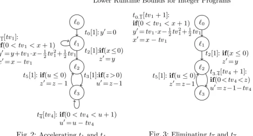
Fig. 3:Eliminatingt1andt4 If we cannot find a metering function or fail to obtain the closed formηit or citfor a simple loopt, then we can simplifytby eliminating temporary variables.
To do so, we fix their values by adding suitable constraints toguard(t). As we are interested in witnesses for maximal computations, we use a heuristic that adds constraintstv =afor temporary variablestv, wherea∈ A(V`) is a suitable upper or lower bound ontv’s values, i.e.,guard(t) impliestv≤aortv≥a. This is repeated until we find constraints which allow us to apply loop acceleration. Note that adding additional constraints to guard(t) isalways sound in our setting.
Theorem 10 (Strengthening). Let t = (`, γ, η, c, `0) ∈ T and ϕ ∈ F(V`).
Then the processor mappingT toT \ {t} ∪ {(`, γ∧ϕ, η, c, `0)} is sound.
Int4 from Fig. 1, γ contains tv > 0. Soγ implies the bound tv ≥1 since tv must be instantiated by integers. Hence, we add the constrainttv = 1. Now the updateu0 =u−tv of the transitiont4 becomesu0 =u−1, and thus,uis a metering function. So after fixingtv = 1,t4can be accelerated similarly to t1.
To simplify the program, we delete a simple looptafter trying to accelerate it. So we just keep the accelerated loop (or none, if acceleration of t still fails after eliminating all temporary variables by strengthening t’s guard). For our example, we obtain the program in Fig. 2 with the accelerated transitions t1,t4. Theorem 11 (Deletion).Fort∈ T, the processor mappingT toT \{t}is sound.
4.2 Chaining Transitions
After trying to accelerate all simple loops of a program, we canchainsubsequent transitionst1, t2by adding a new transitiont1.2that simulates their combination.
Afterwards, the transitionst1andt2can (but need not) be deleted with Thm. 11.
Theorem 12 (Chaining). Lett1= (`1, γ1, η1, c1, `2)andt2= (`2, γ2, η2, c2, `3) with t1, t2∈ T. Letrenbe an injective function renaming the variables inT V`2
to fresh ones and let7t1.2 = (`1, γ1∧ren(η1(γ2)),ren◦η1◦η2, c1+ ren(η1(c2)),
7 For allx∈ PV, ren◦η1◦η2(x) = ren(η1(η2(x))) =η2(x)[x1/η1(x1), . . . , xn/η1(xn), tv1/ren(tv1), . . . ,tvm/ren(tvm)] ifPV={x1, . . . , xn}andT V`2 ={tv1, . . . ,tvm}.
`0
`2
t0.1.2[x+2]:
if(x >0) y0=12x2+12x x0= 0 z0=12x2+12x
t3.4.5[z+1]:
if(z >1) u0= 0 z0=z−1 Fig. 4:Eliminating`1 and`3
`0
`2
t0.1.2[x+2]:
if(x >0) y0= 12x2+12x x0= 0 z0=12x2+12x
t3.4.5[tv·z−12tv2+32tv]:
if(0<tv< z) u0= 0 z0=z−tv
Fig. 5:Acceleratingt3.4.5
`0
`2
t[x2·tv+x·tv−tv2+3tv+2x+4
2 ]:
if(0<tv<12x2+12x) y0=12x2+12x x0= 0 u0= 0
z0= 12x2+12x−tv
Fig. 6:Eliminatingt
3.4.5
`3). Then the processor mapping T toT ∪ {t1.2} is sound. In the new program T ∪ {t1.2}, the temporary variables of`1 are defined to beT V`1∪ren(T V`2).
One goal of chaining isloop elimination of all accelerated simple loops. To this end, we chain all subsequent transitionst0, twheretis a simple loop andt0 is no simple loop. Afterwards, we deletet. Moreover, oncet0 has been chained with all subsequent simple loops, then we also removet0, since its effect is now covered by the newly introduced (chained) transitions. So in our example from Fig. 2, we chaint0 witht1 andt3with t4. The resulting program is depicted in Fig. 3, where we always simplify arithmetic terms and formulas to ease readability.
Chaining also allowslocation elimination by chaining all pairs of incoming and outgoing transitions for a location ` and removing them afterwards. It is advantageous to eliminate locations with just a single incoming transition first.
This heuristic takes into account which locations were the entry points of loops. So for the example in Fig. 3, it would avoid chainingt5andt3.4in order to eliminate
`2. In this way, we avoid constructing chained transitions that correspond to a run from the “middle” of a loop to the “middle” of the next loop iteration.
So instead of eliminating`2, we chaint0.1andt2as well ast3.4andt5to elimi- nate the locations`1and`3, leading to the program in Fig. 4. Here, the temporary variablestv1andtv4vanish since, before applying arithmetic simplifications, the guards oft0.1.2 resp.t3.4.5implytv1=xresp.tv4=z−1.
Our overall approach for program simplification is shown in Alg. 1. Of course, this algorithm is a heuristic and other strategies for the application of the pro- cessors would also be possible. The set S in Steps 3 – 5 is needed to handle locations`with multiple simple loops. The reason is that each transitiont0 with dest(t0) =`should be chained witheach of`’s simple loops before removingt0.
Alg. 1 terminates: In the loop 2.1 – 2.2, each iteration decreases the number of temporary variables in t. The loop 2 terminates since each iteration reduces the number of non-accelerated simple loops. In loop 4, the number of simple loops is decreasing and for loop 6, the number of reachable locations decreases.
The overall loop terminates as it reduces the number of reachable locations.
The reason is that the program does not have simple loops anymore when the algorithm reaches Step 6. Thus, at this point there is either a location` which can be eliminated or the program does not have a path of length 2.
According to Alg. 1, in our example we go back to Step 1 and 2 and applyLoop
Algorithm 1 Program Simplification While there is a path of length 2:
1. ApplyDeletion to transitions whose guard is proved unsatisfiable.
2. While there is a non-accelerated simple loopt:
2.1. Try to applyLoop Acceleration tot.
2.2. If 2.1. failed andtuses temporary variables:
ApplyStrengthening totto eliminate a temporary variable and go to 2.1.
2.3. ApplyDeletion tot.
3. LetS=∅.
4. While there is a simple loopt:
4.1. ApplyChaining to each pairt0, twheresrc(t0)6=dest(t0) =src(t).
4.2. Add all these transitionst0 toS and applyDeletion tot.
5. ApplyDeletion to each transition inS.
6. While there is a location`without simple loops but with incoming and outgoing transitions (starting with locations`with just one incoming transition):
6.1. ApplyChaining to each pairt0, twheredest(t0) =src(t) =`.
6.2. ApplyDeletion to eachtwheresrc(t) =`ordest(t) =`.
Acceleration to transitiont3.4.5. This transition has the metering functionz−1 and its iterated update setsuto 0 andz toz−tv for a fresh temporary variable tv. To computet3.4.5’s iterated costs, we have to find an under-approximation for the solution of the recurrence equationsc(1)=z+ 1 andc(tv+1)=c(tv)+z(tv)+ 1.
After computing the closed formz−tv ofz(tv), the second equation simplifies to c(tv+1) = c(tv)+z−tv+ 1, which results in the closed form cit = c(tv) = tv·z−12tv2+32tv. In this way, we obtain the program in Fig. 5. A final chaining step and deletion of the only simple loop yields the program in Fig. 6.
5 Asymptotic Lower Bounds for Simplified Programs
After Alg. 1, all program paths have length 1. We call such programssimplified and letT be a simplified program throughout this section. Now for anyv∈ Val`0,
max{v(cost(t))|t∈ T,v|=guard(t)}, (5) is a lower bound onT’s derivation heightdhT(v|PV), i.e., (5) is the maximal cost of those transitions whose guard is satisfied byv. So for the program in Fig. 6, we obtain the bound x2·tv+x·tv−tv2+3tv+2x+4
2 for all valuations withv |= 0<tv <
1
2x2+12x. However, such bounds do not provide an intuitive understanding of the program’s complexity and are also not suitable to detect possible attacks. Hence, we now show how to derive asymptotic lower bounds for simplified programs.
These asymptotic bounds can easily be understood (i.e., a high lower bound can help programmers to improve their program to make it more efficient) and they identify potential attacks. After introducing our notion of asymptotic bounds in Sect. 5.1, we present a technique to derive them automatically in Sect. 5.2.
5.1 Asymptotic Bounds and Limit Problems
While dhT is defined on valuations, asymptotic bounds are usually defined for
functions onN. To bridge this gap, we use the common definition of complexity as a function of the size of the input. So the runtime complexity rcT(n) is the maximal cost of any evaluation that starts with a configuration where the sum of the absolute values of all program variables is at mostn.
Definition 13 (Runtime Complexity).Let |v|=P
x∈PV|v(x)| for all valu- ationsv. The runtime complexity rcT :N→R≥0∪ {ω} is defined as rcT(n) = sup{dhT(v)|v∈ Val,|v| ≤n}.
Our goal is to derive an asymptotic lower bound forrcT from a simplified programT. So for the programT in Fig. 6, we would like to derivercT(n)∈Ω(n4).
As usual,f(n)∈ Ω(g(n)) means that there is anm > 0 and an n0 ∈ N such thatf(n) ≥m·g(n) holds for all n≥n0. However, in general, the costs of a transition do not directly give rise to the desired asymptotic lower bound. For instance, in Fig. 6, the costs of the only transition are cubic, but the complexity of the program is a polynomial of degree 4 (sincetv may be quadratic inx).
To infer an asymptotic lower bound from a transitiont∈ T, we try to find an infinite family of valuations vn ∈ Val`0 (parameterized by n ∈ N) where there is an n0 ∈Nsuch that vn |=guard(t) holds for all n≥n0. This implies rcT(|vn|)∈Ω(vn(cost(t))), since for alln≥n0we have:
rcT(|vn|)≥dhT(vn|PV) as |vn|PV|=|vn|
≥vn(cost(t)) by (5)
We first normalize all constraints inguard(t) such that they have the form a >0. Now our goal is to find infinitely many modelsvnfor a formula of the form V
1≤i≤k(ai >0). Obviously, such a formula is satisfied if all termsai are positive constants or increase infinitely towardsω. Thus, we introduce a technique which tries to find out whether fixing the valuations of some variables and increasing or decreasing the valuations of others results in positive resp. increasing valuations ofa1, . . . , ak. Our technique operates on so-calledlimit problems {a•11, . . . , a•kk} whereai ∈ A(V`0) and •i ∈ {+,−,+!,−!}. Here, a+ (resp. a−) means thata grows towardsω(resp.−ω) anda+! (resp.a−!) means thatahas to be a positive (resp. negative) constant. So we represent guard(t) by an initial limit problem {a•11, . . . , a•kk} where •i ∈ {+,+!} for all 1 ≤ i ≤ k. We say that a family of valuationsvn is asolution to a limit problemS iffvn “satisfies”S for large n.
To define this notion formally, for any function f : N → R we say that limn7→ωf(n) = ω (resp. limn7→ωf(n) = −ω) iff for every m ∈ Z there is an n0 ∈N such that f(n) ≥m (resp. f(n) ≤m) holds for all n ≥n0. Similarly, limn7→ωf(n) =miff there is ann0such thatf(n) =mholds for alln≥n0. Definition 14 (Solutions of Limit Problems).For any function f :N→R and any • ∈ {+,−,+!,−!}, we say thatf satisfies •iff
limn7→ωf(n) =ω, if•= + ∃m∈Z. limn7→ωf(n) =m >0,if •= +!
limn7→ωf(n) =−ω,if•=− ∃m∈Z. limn7→ωf(n) =m <0,if •=−!
A familyvn of valuations is a solutionof a limit problem S iff for every a•∈S, the functionλn.vn(a)satisfies•. Here, “λn.vn(a)” is the function fromN→R that maps anyn∈Ntovn(a).
Example 15 (Bound for Fig. 6).In Fig. 6 whereguard(t) is 0<tv < 12x2+12x, the family vn with vn(tv) = 12n2+ 12n−1,vn(x) = n, and vn(y) = vn(z) = vn(u) = 0 is a solution of the initial limit problem{tv+,(12x2+ 12x−tv)+!)}.
The reason is that the functionλn. vn(tv) that maps anyn ∈N to vn(tv) =
1
2n2+12n−1 satisfies +, i.e., limn7→ω(12n2+12n−1) =ω. Similarly, the function λn. vn(12x2+12x−tv) = λn. 1 satisfies +!. Sect. 5.2 will show how to infer such solutions of limit problems automatically. Thus, there is an n0 such that vn |=guard(t) holds for alln≥n0. Hence, we get the asymptotic lower bound rcT(|vn|)∈Ω(vn(cost(t))) =Ω(18n4+14n3+78n2+74n) =Ω(n4).
Theorem 16 (Asymptotic Bounds for Simplified Programs). Given a transition t of a simplified program T with guard(t) = a1 > 0∧ · · · ∧ak > 0, let the family vn be a solution of an initial limit problem {a•11, . . . , a•kk} with
•i∈ {+,+!} for all1≤i≤k. ThenrcT(|vn|)∈Ω(vn(cost(t))).
Of course, if T has several transitions, then we try to take the one which results in the highest lower bound. Moreover, one should extend the initial limit problem{a•11, . . . , a•kk}by cost(t)+. In this way, one searches for valuationsvn
wherevn(cost(t)) depends onn, i.e., where the costs are not constant.
The costs areunbounded (i.e., they only depend on temporary variables) iff the initial limit problem{a•11, . . . , a•kk,cost(t)+}has a solutionvnwherevn(x) is constant for allx∈ PV. Then we can even inferrcT(n)∈Ω(ω). For instance, after chaining the transitiontof Ex. 9 with the transition from the start location (see Ex. 5), the resulting initial limit problem{x+!,tv+,(tv·y+ 1)+}has the solution vn withvn(x) =vn(y) = 1 and vn(tv) =n, which impliesrcT(n)∈Ω(ω).
If the costs are not unbounded, we say that they depend on x ∈ PV iff the initial limit problem{a•11, . . . , a•kk,cost(t)+}has a solutionvnwherevn(y) is constant for ally∈ PV \{x}. Ifxcorresponds to a “secret”, then the program can be subject to side-channel attacks. For example, in Ex. 15 we havevn(cost(t)) =
1
8n4+14n3+78n2+74n. Sincevnmaps all program variables exceptxto constants, the costs of our program depend on the program variablex. So ifxis “secret”, then the program is not safe from side-channel attacks.
Thm. 16 results in bounds of the form “rcT(|vn|)∈Ω(vn(c))”, which depend on thesizes|vn|. Letf(n) =rcT(n),g(n) =|vn|, and letΩ(vn(c)) have the form Ω(nk) orΩ(kn) for ak∈N. Moreover for allx∈ PV, letvn(x) be a polynomial of at most degree m, i.e., let g(n) ∈ O(nm). Then the following observation from [15] allows us to infer a bound for rcT(n) instead of rcT(|vn|).
Lemma 17 (Bounds for Function Composition). Let f : N→ R≥0 and g : N→ N where g(n) ∈ O(nm) for some m∈ N\ {0}. Moreover, let f(n) be weakly and letg(n)be strictly monotonically increasing for large enoughn.
• Iff(g(n))∈Ω(nk)withk∈N, thenf(n)∈Ω(nmk).
• Iff(g(n))∈Ω(kn)withk∈N, thenf(n)∈Ω(km√n).
Example 18 (Bound for Fig. 6 Continued). In Ex. 15, we inferredrcT(|vn|)∈ Ω(n4) where vn(x) = n and vn(y) = vn(z) = vn(u) = 0. Hence, we have
|vn|=n∈ O(n1). By Lemma 17, we obtainrcT(n)∈Ω(n41) =Ω(n4).
Example 19 (Non-Polynomial Bounds).LetT={(`0, x=y2,id, y, `)}. By Def. 14, the familyvn with vn(x) =n2 and vn(y) =n is a solution of the initial limit problem{(x−y2+1)+!,(y2−x+1)+!, y+}. Due to Thm. 16, this provesrcT(|vn|)∈ Ω(n). As|vn|=n2+n∈ O(n2), Lemma 17 results inrcT(n)∈Ω(n12).
5.2 Transformation of Limit Problems
A limit problemSistrivial iff all terms inSare variables and there is no variable xwithx•1, x•2 ∈S and•16=•2. For trivial limit problemsS we can immediately obtain a particular solution vSn which instantiates variables “according toS”.
Lemma 20 (Solving Trivial Limit Problems). LetS be a trivial limit prob- lem. Then vSn is a solution ofS where for all n∈N,vSn is defined as follows:
vSn(x) = n,if x+∈S vSn(x) = 1,if x+!∈S vSn(x) = 0,otherwise vSn(x) =−n,if x−∈S vSn(x) =−1,if x−!∈S
For instance, ifV`0 ={x, y,tv} andS ={x+, y−!}, thenS is a trivial limit problem andvSn withvSn(x) =n,vSn(y) =−1, andvSn(tv) = 0 is a solution forS.
However, in general the initial limit problem S = {a•11, . . . , a•kk,cost(t)+} is not trivial. Therefore, we now define a transformation to simplify limit problems until one reaches a trivial problem. With our transformation,S S0 ensures that each solution ofS0 also gives rise to a solution of S.
IfS containsf(a1, a2)• for some standard arithmetic operationf like addi- tion, subtraction, multiplication, division, and exponentiation, we use a so-called limit vector (•1,•2) with •i ∈ {+,−,+!,−!} to characterize for which kinds of arguments the operation f is increasing (if• = +) resp. decreasing (if •=−) resp. a positive or negative constant (if • = +! or • = −!).8 Then S can be transformed into the new limit problemS\ {f(a1, a2)•} ∪ {a•11, a•22}.
For example, (+,+!) is an increasing limit vector for subtraction. The reason is thata1−a2is increasing ifa1is increasing anda2is a positive constant. Hence, our transformation allows us to replace (a1−a2)+ bya+1 anda+2!.
To define limit vectors formally, we say that (•1,•2) is anincreasing (resp.de- creasing)limit vector forf iff the functionλn. f(g(n), h(n)) satisfies + (resp.−) for any functionsgandhthat satisfy•1 and•2, respectively. Here, “λn. f(g(n), h(n))” is the function fromN→Rthat maps anyn∈Nto f(g(n), h(n)). Simi- larly, (•1,•2) is apositive (resp. negative)limit vector forf iffλn. f(g(n), h(n)) satisfies +!(resp.−!) for any functionsgandhthat satisfy•1and•2, respectively.
With this definition, (+,+!) is indeed an increasing limit vector for subtraction, since limn7→ωg(n) =ωand limn7→ωh(n) =mwithm >0 implies limn7→ω(g(n)− h(n)) =ω. In other words, ifg(n) satisfies + andh(n) satisfies +!, then g(n)− h(n) satisfies + as well. In contrast, (+,+) is not an increasing limit vector for subtraction. To see this, consider the functionsg(n) =h(n) =n. Bothg(n) and h(n) satisfy +, whereasg(n)−h(n) = 0 does not satisfy +. Similarly, (+!,+!) is
8 To ease the presentation, we restrict ourselves to binary operationsf. For operations of aritym, one would need limit vectors of the form (•1, . . . ,•m).
not a positive limit vector for subtraction, since forg(n) = 1 andh(n) = 2, both g(n) andh(n) satisfy +!, butg(n)−h(n) =−1 does not satisfy +!.
Limit vectors can be used to simplify limit problems, cf. (A) in the following definition. Moreover, for numbers m∈Z, one can easily simplify constraints of the formm+! andm−! (e.g., 2+! is obviously satisfied since 2>0), cf. (B).
Definition 21 ( ). Let S be a limit problem. We have:
(A) S∪ {f(a1, a2)•} S∪ {a•11, a•22} if• is+(resp. −,+!,−!) and(•1,•2)is an increasing (resp. decreasing, positive, negative) limit vector forf (B) S∪ {m+!} S if m∈Zwith m >0,S∪ {m−!} S ifm <0
Example 22 (Bound for Fig. 6 Continued). For the initial limit problem from Ex. 15, we have {tv+,(12x2 + 12x−tv)+!} {tv+,(12x2 + 12x)+!,tv−!} {tv+,(12x2)+!,(12x)+!,tv−!} ∗ {tv+, x+!,tv−!} using the positive limit vector (+!,−!) for subtraction and the positive limit vector (+!,+!) for addition.
The resulting problem in Ex. 22 is not trivial as it containstv+andtv−!, i.e., we failed to compute an asymptotic lower bound. However, if we substitutetv with its upper bound12x2+12x−1, then we could reduce the initial limit problem to a trivial one. Hence, we now extend by allowing to apply substitutions.
Definition 23 ( Continued). LetS be a limit problem and let σ : V`0 → A(V`0)be a substitution such thatxdoes not occur inxσ and v(xσ)∈Z for all valuationsv∈ Val`0 and all x∈ V`0. Then we have9
(C) S σSσ
Example 24 (Bound for Fig. 6 Continued). For the initial limit problem from Ex. 15, we now have10{tv+,(12x2+12x−tv)+!} [tv/12x2+12x−1]{(12x2+12x−1)+, 1+!} {(12x2+12x−1)+} {(12x2+12x)+,1+!} ∗{x+}, which is trivial.
Although Def. 23 requires that variables may only be instantiated by integer terms, it is also useful to handle limit problems that contain non-integer terms.
Example 25 (Non-Integer Metering Functions Continued). After chaining the accelerated transition of Ex. 8 with the transition from the start location, for the resulting initial limit problem we get {tv+,(12x−tv+ 1)+!,(tv+ 1)+} 2 {tv+,(12x−tv+ 1)+!} [x/2tv−1]{tv+,12+!} {tv+,1+!,2+!} 2{tv+}, using the positive limit vector (+!,+!) for division. This allows us to inferrcT(n)∈Ω(n).
However, up to now we cannot prove that, e.g., a transitiontwithguard(t) = x2−x > 0 and cost(t) = x has a linear lower bound, since (+,+) is not an increasing limit vector for subtraction. To handle such cases, the following rules allow us to neglect polynomial sub-expressions if they are “dominated” by other polynomials of higher degree or by exponential sub-expressions.
Definition 26 ( Continued).LetS be a limit problem, let± ∈ {+,−}, and leta, b, e∈ A({x})be (univariate) polynomials. Then we have:
(D)S∪ {(a±b)•} S∪ {a•}, if• ∈ {+,−}, and ahas a higher degree thanb
9 The other rules for are implicitly labeled with the identical substitutionid.
10σ= [tv/12x2+12x−1] satisfies the conditionv(yσ)∈Zfor allv∈ Val`0 andy∈ V`0.
(E) S∪ {(ae±b)+} S∪ {(a−1)•, e+}, if • ∈ {+,+!}.
Thus,{(x2−x)+} {(x2)+}={(x·x)+} {x+}by the increasing limit vector (+,+) for multiplication. Similarly, {(2x−x3)+} {(2−1)+!, x+} {x+}.
Rule (E) can also be used to handle problems like (ae)+ (by choosingb= 0).
Thm. 27 states that is indeed correct. When constructing the valuation from the resulting trivial limit problem, one has to take the substitutions into account which were used in the derivation. Here, (vn◦σ)(x) stands forvn(σ(x)).
Theorem 27 (Correctness of ). IfS σS0 and the familyvnis a solution ofS0, thenvn◦σis a solution of S.
Example 28 (Bound for Fig. 6 Continued).Ex. 24 leads to the solutionv0n◦σof the initial limit problem for the program from Fig. 6 whereσ= [tv/12x2+12x−1], v0n(x) =n, andv0n(tv) =v0n(y) =v0n(z) =v0n(u) = 0. Hence,v0n◦σ=vn where vn is as in Ex. 15. As explained in Ex. 18, this provesrcT(n)∈Ω(n4).
So we start with an initial limit problem S = {a•11, . . . , a•kk,cost(t)+} that represents guard(t) and requires non-constant costs, and transform S with into a trivialS0, i.e.,S σ1 . . . σmS0. For automation, one should leave the•i
in the initial problemS open, and only instantiate them by a value from{+,+!} when this is needed to apply a particular rule for the transformation . Then the resulting familyvSn0 of valuations gives rise to a solutionvSn0◦σm◦. . .◦σ1
ofS. Thus, we havercT(|vSn0◦σ|)∈Ω(vSn0(σ(cost(t)))), whereσ=σm◦. . .◦σ1, which leads to a lower bound forrcT(n) with Lemma 17.
Our implementation uses the following strategy to apply the rules from Def. 21, 23, 26 for . Initially, we reduce the number of variables by propagating bounds implied by the guard, i.e., ifγ =⇒ x≥aorγ =⇒x≤afor somea∈ A(V`0\{x}), then we apply the substitution [x/a] to the initial limit problem by rule (C). For example, we simplify the limit problem from Ex. 19 by instantiatingxwithy2, as the guard of the corresponding transition implies x= y2. So here, we get {(x−y2+ 1)+!,(y2−x+ 1)+!, y+} [x/y2]{1+!, y+} {y+}. Afterwards, we use (B) and (D) with highest and (E) with second highest priority. The third priority is trying to apply (A) to univariate terms (since processing univariate terms helps to guide the search). As fourth priority, we apply (C) with a substitution [x/m] if x+! orx−! inS, where we use SMT solving to find a suitablem ∈Z. Otherwise, we apply (A) to multivariate terms. Since is well founded and, except for (C), finitely branching, one may also backtrack and explore alternative applications of . In particular, we backtrack if we obtain a contradictory limit problem. Moreover, if we obtain a trivialS0wherevSn0(σ(cost(t))) is a polynomial, butcost(t) is a polynomial of higher degree or an exponential function, then we backtrack to search for other solutions which might lead to a higher lower bound.
However, our implementation can of course fail, since solvability of limit problems is undecidable (due to Hilbert’s Tenth Problem).
6 Experiments and Conclusion
We presented the first technique to infer lower bounds on the worst-case run-
time complexity of integer programs, based on a modular program simplification framework. The main simplification technique isloop acceleration, which relies onrecurrence solving andmetering functions, an adaptation of classical ranking functions. By eliminating loops and locations viachaining, we eventually obtain simplified programs. We presented a technique to inferasymptotic lower bounds from simplified programs, which can also be used to find vulnerabilities.
Our implementationLoAT(“Lower Bounds Analysis Tool”) is freely available at [23]. It was inspired byKoAT[8], which alternates runtime- and size-analysis to inferupper bounds in a modular way. Similarly,LoATalternates runtime-analysis and recurrence solving to transform loops to loop-free transitions independently.
LoAT uses the recurrence solverPURRS[4] and the SMT solverZ3[10].
We evaluatedLoATon the benchmarks [5] from the evaluation of [8]. We omit- ted 50 recursive programs, since our approach cannot yet handle recursion. As we know of no other tool to compute worst-case lower bounds for integer programs, we compared our results with the asymptotically smallest results of leading tools for upper bounds:KoAT,CoFloCo[14],Loopus[26],RanK[2]. We did not compare withPUBS[1], since the cost relations analyzed byPUBSsignificantly differ from the integer programs handled by LoAT. Moreover, asPUBS computesbest-case lower bounds, such a comparison would be meaningless since the worst-case lower bounds computed byLoATare no valid best-case lower bounds. We used a timeout of 60 seconds. In the following, we disregard 132 examples where rcT(n)∈ O(1) was proved since there is no non-trivial lower bound in these cases.
rcT(n) Ω(1)Ω(n)Ω(n2)Ω(n3)Ω(n4)EXP Ω(ω)
O(1) (132) – – – – – –
O(n) 45 125 – – – – – O(n2) 9 18 33 – – – – O(n3) 2 – – 3 – – – O(n4) 1 – – – 2 – –
EXP – – – – – 5 –
O(ω) 57 31 3 – – – 173
LoATinfers non-trivial lower bounds for 393 (78%) of the remaining 507 ex- amples. Tight bounds (i.e., the lower and the upper bound coincide) are proved in 341 cases (67%). Whenever an exponential upper bound is proved, LoATalso proves an exponential lower
bound (i.e.,rcT(n)∈Ω(kn) for somek >1). In 173 cases,LoATinfers unbounded runtime complexity. In some cases, this is due to non-termination, but for this particular goal, specialized tools are more powerful (e.g., wheneverLoATproves unbounded runtime complexity due to non-termination, the termination analyzer T2 [7] shows non-termination as well). The average runtime of LoAT was 2.4 seconds per example. These results could be improved further by supplementing LoATwith invariant inference as implemented in tools like APRON [20]. For a detailed experimental evaluation of our implementation as well as the sources and a pre-compiled binary of LoATwe refer to [16].
AcknowledgmentsWe thank S. Genaim and J. B¨oker for discussions and comments.
References
1. Albert, E., Genaim, S., Masud, A.N.: On the inference of resource usage upper and lower bounds. ACM Transactions on Computational Logic 14(3) (2013)
2. Alias, C., Darte, A., Feautrier, P., Gonnord, L.: Multi-dimensional rankings, program termination, and complexity bounds of flowchart programs. In: Proc. SAS ’10. pp.
117–133. LNCS 6337 (2010)