Sensitivity of the anomalous Hall effect to disorder correlations
I. A. Ado,1I. A. Dmitriev,2,3,4P. M. Ostrovsky,3,5and M. Titov1,6
1Radboud University, Institute for Molecules and Materials, NL-6525 AJ Nijmegen, The Netherlands
2University of Regensburg, Department of Physics, 93040 Regensburg, Germany
3Max Planck Institute for Solid State Research, Heisenbergstr. 1, 70569 Stuttgart, Germany
4A. F. Ioffe Physico-Technical Institute, 194021 St. Petersburg, Russia
5L. D. Landau Institute for Theoretical Physics RAS, 119334 Moscow, Russia
6ITMO University, Saint Petersburg 197101, Russia (Received 24 October 2017; published 27 December 2017)
Both longitudinal and anomalous Hall conductivities are computed in the model of two-dimensional Dirac fermions with a mass in the presence of weak Gaussian spin-independent disorder with an arbitrary correlation function. The anomalous Hall conductivity is shown to be highly sensitive to the correlation properties of the random potential, such as the correlation length, while it remains independent of the integral disorder strength.
This property extends beyond the Dirac model making the anomalous Hall effect an interesting tool to probe disorder correlations.
DOI:10.1103/PhysRevB.96.235148
I. INTRODUCTION
The anomalous Hall effect (AHE) is one of the most direct manifestations of spin-orbit interaction in magnetic conductors. The effect has been discovered as early as in 1881 by Edwin Hall who observed a transverse voltage in ferromagnetic iron as a reaction to electric current applied [1].
In that respect, the AHE is completely analogous to the usual Hall effect but can be observed in much weaker magnetic fields that are only needed to magnetize the conductor [2]. A closely related phenomenon of the AHE in antiferromagnetic and paramagnetic systems has, however, received a widespread attention only recently [3–5].
The interest to spin-orbit induced phenomena has increased dramatically following the discovery of topological insulators and Weyl semimetals [6–10]. Moreover, the on-going develop- ment in the fields of spintronics [11–14], cold atoms [15–17], chiral superconductivity [18–21], and magnetization dynamics [22–26] call for deeper understanding of the microscopic mechanisms of spin-orbit assisted transport [27–29]. The detailed interpretation of the AHE measurements may pro- vide valuable information regarding exchange and spin-orbit coupling that is of key importance for applications.
Despite the long and rich history of the field [2], it has been recently found by the authors [30,31] that previous treatments of AHE were fundamentally incomplete. Indeed, in many models and materials, the AHE conductivity is subleading in a large metal parameter εFτ compared to the longitudinal conductivity (hereεF is the Fermi energy). This is reflected in the fact that the anomalous Hall conductivity does not depend on the electron scattering timeτ and is of the order of intrinsic contribution, which is manifestly disorder- independent. It appears, nevertheless, that the presence of impurities essentially modify the AHE including its sign [31], even though the disorder strength is canceling out from the result.
It has been demonstrated in Refs. [30,31] that the conven- tional “noncrossing approximation” (NCA) employed in the diagrammatic calculation of longitudinal conductivityσxx is not applicable to AHE. In addition to ladder diagrams with
noncrossing impurity lines that describe electron diffusion, the AHE conductivityσxy requires additional terms that are represented by diagrams with two intersecting impurity lines (the so-called X and diagrams [30,31]). Very recently, the same crossed diagrams have been shown to play a key role for the AHE on the surface of topological Kondo insulators [32], for the Kerr effect in chiral p-wave superconductors [33], and for the spin Hall effect in the presence of strong impurities [34]. From the physics point of view, such terms represent an essential part of the full cross section describing skew scattering on pairs of closely positioned impurities. The important role of such rare impurity configurations in the theory of AHE calls for a detailed investigation of the effects of disorder correlations that is the main subject of the present publication.
For two basic microscopic models of AHE [2], the anomalous Hall conductivityσxy has been shown to depend dramatically on the inclusion of X and diagrams [30,31].
More specifically, in 2D Rashba ferromagnet, the AHE conductivity does not vanish in the metallic limit solely due to these contributions [31], in sharp contrast to the well-known vanishing NCA result [35,36]. In the case of massive Dirac fermions, which represent the simplest model featuring the AHE, the X and diagrams almost cancel out the NCA contribution [30]. In the model with weak white noise disorder, the anomalous Hall conductivityσxydecays asεF−3in the metal regime instead ofε−1F given by the NCA [37,38].
Given that the AHE is so sensitive to the scattering on rare impurity configurations, it is interesting to establish whether and how these results modify for more general disorder models with finite correlation length. Here we extend the analytic approach of Refs. [30,31,37] to massive Dirac fermions subject to weak spin-independent Gaussian disorder with an arbitrary pair correlator of the random potential [39]. In real systems, the disorder potential is almost always correlated on the scale of the Fermi wavelength (due to the Coulomb screening). At the same time, the AHE is proven to be greatly sensitive to such short distances due to the leading role of the skew scattering on closely positioned impurities [30,31]. Thus the sensitivity of
the AHE in metals to disorder correlations extends far beyond the model considered below.
As might have been expected, our results reveal strong sensitivity of the AHE conductivity to the correlation prop- erties of disorder. In particular, it turns out that a strong mutual cancellation of intrinsic and extrinsic contributions for the model of Dirac fermions [30] is a specific feature of uncorrelated disorder. In the opposite limit of smooth disorder, which corresponds to small-angle scattering, the intrinsic and extrinsic contributions toσxyhave the same sign. In this case, the total Hall conductivity at large energiesσxy∝ε−F1is given by the intrinsic conductivity multiplied by a factor of three.
Depending on the functional form of the pair correlator, the AHE conductivity may feature a nonmonotonic dependence on the correlation length and possess maximal values in the crossover region between the above limits of white-noise and smooth disorder.
The paper is organized as follows. In Sec. II, we intro- duce the model and calculate the disorder-averaged Green’s functions. In Sec.III, we obtain general expressions for the longitudinal and anomalous Hall conductivities in terms of the angular moments of the disorder correlation function. In Sec.IV, these general results are applied to generic limiting cases of white-noise and smooth disorder. SectionVillustrates the crossover between the two limits for two specific models of disorder. Section VI contains summary and conclusions.
Certain technical details of calculations and complementary information are presented in AppendicesAandB.
II. MODEL, DISORDER-AVERAGED GREEN’S FUNCTIONS
A. Model
The model of massive Dirac fermions in two dimensions has been proposed by Haldane [40] as the simplest toy model to illustrate the quantum anomalous Hall effect. The latter arises when the chemical potential is placed in the band gap. In this paper we focus on the metal regime, i.e., on the case of the chemical potential situated within the band. In particular, we compute both the longitudinal and Hall conductivity for the model of massive Dirac fermions in two dimensions, which is described by the Hamiltonian
H=H0+V(r), H0=vσp+mσz, (1) where V(r) denotes a weak correlated Gaussian random potential,σ =(σx,σy) stands for the vector of Pauli matrices, p=(px,py) is the momentum operator,vis the characteristic velocity, and m is the bare “mass” of relativistic fermions.
The random potential is shifted to a vanishing mean value V(r) =0. Its statistical properties are defined by the pair correlator
V(r)V(r) =2πα(r−r), (2) where the angular brackets denote the averaging over the disorder realizations. In diagrammatic language, such a cor- relator is visualized by a disorder line, which corresponds to the propagator 2π α(q)=2π
d2rα(r)e−iq rthat depends on the transferred momentum q. Throughout the paper we let
¯
h=v=1, hence all momenta are measured in the units of energy.
The model of Eq. (1) is characterized by the broken time- reversal invariance hence it gives rise to a finite Hall response.
In condensed matter context, the Hamiltonian of the type (1) can be used as an effective model [41–44] to describe the surface of the 3D topological insulator [24,45] (see, however, Ref. [46] for the detailed discussion). One may also view the model of Eq. (1) as the single-valley projection of the full Hamiltonian describing a graphene/hBN heterostructure [47].
In the latter case, however, the Pauli matricesσα act in the isospin space while the true time-reversal invariance of the Hamiltonian is preserved. This means that the AHE for the model of Eq. (1) corresponds to the valley Hall effect in a graphene/hBN bilayer.
The quantum anomalous Hall effect, studied by Haldane [40] in the model of Eq. (1), is manifestly independent of the disorder potential and is taking place for the chemical potential placed within the band gap. To study transport properties outside the gap, one needs to take into account the scattering on impurities both in the longitudinal and in the anomalous Hall conductivity [48]. The missing leading-order terms in the theory of AHE have been discovered by the authors only recently [30].
In what follows we compute the components of the conductivity tensor to the leading order inα. In order to do so, it is sufficient to know the disorder scattering probability only for the states belonging to the Fermi surface. The spectrum ofH0 consists of two branchesε±(p)= ±
p2+m2separated by a gap of size 2|m|. Without loss of generality, we assume that the Fermi energyεbelongs to the upper bandε > m >0 so that p0=√
ε2−m2is the corresponding Fermi momentum. The transferred momentum q =2p0sin(φ/2) is, then, uniquely expressed by the scattering angle φ. With these definitions we express the angle-dependent scattering probability as
α(φ)≡α[q →2p0sin(φ/2)]=α0+2 ∞ n=1
αncos(nφ), (3) where the parameters αn stand for the angular harmonics of the scattering probability. The notation α(φ) is used interchangeably withα(q) below. The particular limit of white- noise disorder, α(r)=αδ(r), which has been investigated in Ref. [30], corresponds to αn=αδn,0, where δn,m is the Kronecker symbol.
B. Self-energy and average Green’s functions
The main building block of diagrammatic calculations below is the Green’s function averaged over disorder con- figurations in the Born approximation. The latter is defined by the corresponding self-energy with a logarithmically diverging real part, which is absorbed in the renormalization of energy and mass, and with a finite imaginary part. The latter is set by the difference between the retarded and advanced self-energy
Rp −Ap = d2p
2π α(p− p)[GR(p)−GA(p)], (4) where the Green’s functions can be taken in the clean limit. The bare Green’s functions [which correspond to the Hamiltonian
H0in the Eq. (1)] yield
GR0(p)−GA0(p)= −2π i[ε+mσz+σp]δ
p2−p02 ,
(5) where the presence of delta-function bounds the particle momentum pto the Fermi surface.
We only need to know the self-energy for momenta at the Fermi surface,p=p0, consequently we find the result
Rp −Ap = −iπ dφ
2π α(φ−φ)
×(ε+mσz+p0σxcosφ+p0σysinφ)
= −iπ(α0(ε+mσz)+α1σp), (6) which depends only on the first two harmonics of the disorder correlator.
Using the self-energy of Eq. (6), we obtain the averaged Green’s function in the form
GR,A(p)=ε±iγ+(m∓iμ)σz+(1∓iζ)σp ε2−m2−p2±i , (7) where we introduce the parameters
=2(εγ+mμ+ζp2)=π(ε2(α0+α1)+m2(α0−α1)), γ =π α0ε/2, μ=π α0m/2, ζ =π α1/2, (8) with the expression for taken atp=p0. This is justified since the imaginary part of the Green’s function denominator is relevant only at the mass shell.
The singular part of the average Green function comes from the Fermi surface and can be obtained from Eq. (7) via projection on the corresponding spectral branch. For the Fermi energyε > m, it is given by
GR,A+ (p)= |φφ| ε−
m2+p2+i/2τ, (9) where we introduced the scattering rate 1/τ =|p=p0/εand the corresponding eigenstate
|φ = 1
√2ε
√ε+m
√ε−m eiφ
, (10)
where the angle φ specifies the direction of the momentum (taken at the Fermi surface).
The scattering rate 1/τ in Eq. (9) is expressed by the Fermi golden rule as
1/τ =2π ε[α(φ)(φ)]φ, (φ−φ)≡ |φ|φ|2, (11) where the square brackets denote the angular averaging
[u(φ)]φ ≡ dφ
2π u(φ), (12) and we introduce the so-called Dirac factor
(φ)=cos2φ 2 +m2
ε2 sin2φ
2, (13)
which reflects the structure of the eigenstates. The expressions (4)–(13) provide the basis for the diagrammatic analysis of the conductivity tensor, which we undertake in the next section.
III. CONDUCTIVITY TENSOR FOR CORRELATED WEAK GAUSSIAN DISORDER
A. General remarks
To compute the dc conductivity tensor for the system described by Eqs. (1)–(3), we employ the Kubo-Streda formula [49] in the limit of zero temperature and for the Fermi energy,ε > m >0, belonging to the conduction band. In this paper, we generalize the formalism developed in Ref. [30]
to the case of correlated weak disorder. Unlike Ref. [30], where the computation has been performed in the real space representation for the case of uncorrelated (white noise) disorder, we use here the momentum representation, which is more appropriate for dealing with correlated disorder.
The Kubo-Streda formula for the conductivity tensor consists of two terms traditionally denoted as ˆσI and ˆσII. The first term ˆσI describes the contribution of conduction electrons with momenta at the Fermi surface. The second term accounts for the contribution to the nondiagonal components of the conductivity tensor σxy= −σyx that stems from the entire Fermi sea. In particular, the second contribution can be expressed as σxyII =ec ∂n/∂B|B→0 as the derivative of the total electron concentrationnwith respect to an external perpendicular magnetic fieldBtaken in the limitB→0 [49].
For the Fermi energy inside the spectral gap,|ε|< m, the longitudinal conductivityσxx vanishes, while the entire Hall conductivity is given by [40,48,50],
σxy=σxyII = −e2/4π, (14) which remains insensitive to a weak disorder. The result of Eq. (14) is often referred to as the quantum anomalous Hall effect.
As the Fermi energy is increased above the gap,ε > m, the contributionσxyII quickly becomes negligible in comparison to the Fermi surface contribution σxyI . In this case, the conductivity tensor is given by
σijI = e2
2π TrσiGRσjGA, (15) where GA andGR stand for the exact Green’s functions in the presence of disorder. The angular brackets denote the averaging over disorder realizations defined by Eq. (2). Let us remind that in our units ( ¯h=1 andv=1), the conductance quantum e2/ h reads e2/2π, while the components of the current operator are given by the Pauli matrices σx,y. In the following, we compute the conductivity tensor (15) as a function of the angular harmonicsαnof the disorder potential correlator given in Eq. (3) to the leading order in the disorder strength.
We start in Sec. III B with the longitudinal conductivity σxx=σyy=O(α−n1) that is proportional to the scattering time τ. The averaging procedure in this case is reduced to the computation of the standard ladder diagrams with noncrossing impurity lines as illustrated in Figs.1(a)and1(e).
The dominant contribution toσxx is determined entirely by the states belonging to the Fermi surface. To perform the calculation in the leading order α−n1∝τ, it is sufficient to know only the singular part of the Green’s functions of Eq. (9), which is represented by thin lines in Fig.1.
x x
x y
x y
x y
(a)
(c)
(b)
(d)
(e)
FIG. 1. Diagrams representing the leading contributions to the longitudinal conductivityσxx=O(α−1n ) (a) and the anomalous Hall conductivityσxy=O(α0n) [(b), (c), and (d)]. The latter is the sum of the noncrossing contributionσxync[(b)] and crossing contributions represented by X (c) and (d) diagrams, which include a pair of crossed impurity lines (dashed lines). Thin solid lines correspond to Green’s functions (9) projected to the Fermi surface, while thick solid lines correspond to full disorder-averaged Green’s functions (7). Vertex correction (e) involves the sum of ladder diagrams with projected Green functionsG+only.
The same approximation applied to the anomalous Hall conductivityσxyreturns a vanishing result. This is intuitively clear since the full projection to one of the bands restores the time-reversal symmetry of the model. To obtain a finite result forσxy, one needs to take into account states that lay far from the Fermi surface. As a result, the AHE has a parametric smallnessσxy=O(α0n) as compared toσxx=O(αn−1). A part ofσxycomes from noncrossing diagrams in Fig.1(b), where, in comparison to Fig.1(a), any single pair of the projected Green functions (9) has to be replaced by full Green functions (7) (thick lines in Fig.1), which include contribution of states far away from the Fermi surface. The corresponding part of σxyis calculated in Sec.III C.
The noncrossing diagrams in Fig.1(b)do not exhaust all contributions to the AHEσxy even in the leading order with respect to the disorder strength. As demonstrated in Ref. [30], a complete description requires inclusion of additional diagrams in Figs.1(c)and1(d), which involve a single pair of crossed impurity lines. It is well known that crossing of impurity lines leads to a parametric smallness since the momentum conservation law does not enable bounding of all momenta to the Fermi surface. But in the case of anomalous Hall conductivity one of the momenta needs to be away from the Fermi surface even in the noncrossing diagrams, Fig.1(b). As discussed in more details in Refs. [30–33], in this situation, crossing of impurity lines in Figs. 1(c) and 1(d) does not produce any additional smallness with respect to Fig.1(b). The corresponding contribution toσxyis calculated in Sec.III D.
B. Longitudinal conductivity
The longitudinal conductivityσxxin the leading order inαn
is given by the sum of ladder diagrams illustrated in Fig.1(a).
The result can be written as σxx= e2
2π 2π
0
dφ 2π
∞
0
p dp
2π Tr(GA+(p) ¯σxGR+(p)σx), (16) where ¯σx represents the current operator, dressed by the impurity ladder as shown in Fig.1(e). In what follows, we often do not specify the integration limits explicitly since they are always the same as in Eq. (16).
As have been already mentioned, the calculation of the longitudinal conductivity to the leading order in disorder strength can be preformed entirely with projected Green’s functions given by Eq. (9). This is not the case for the AHE as will be explained in the next section.
Let us first compute the matrix elementφ|σ¯x|φ, which represents the disorder-dressed current vertex. The projected bare current operator reads
φ|σx|φ = p0
ε cosφ, (17) where the ratiop0/εis the Fermi velocity. This matrix element is transformed as
p0
ε cosφ→ p0 ε
p dp dφ 2π
φ|φα(φ−φ)φ|φcosφ (ε−
m2+p2)2+1/4τ2
=p0τ
dφα(φ−φ)(φ−φ) cosφ
= p0
ε cosφ[α(φ)(φ) cosφ]φ
[α(φ)(φ)]φ
, (18)
after dressing by a single impurity line. Summing up the entire ladder results in the fully dressed projected current,
φ|σ¯x|φ = p0
ε cosφ [α(φ)(φ)]φ
[α(φ)(φ)(1−cosφ)]φ
= p0τtr
ετ cosφ, (19)
which defines the transport scattering rate 1
τtr =2π ε[α(φ)(φ)(1−cosφ)]φ
= π
2ε(ε2(α0−α2)+m2(3α0−4α1+α2)), (20) which depends on the first three harmonics of the random potential. We shall remind here that the scattering timeτis the average time between two scattering events, while the transport timeτtris the characteristic time of momentum relaxation. In the limit of very smooth disorder, whenαnis a slow function of n, the transport time may exceed the scattering time by orders of magnitude since the small angle scattering dominates.
It is instructive to define the following object:
Jx(φ)=
p dp
2π GA+(p) ¯σxGR+(p)
= p0τtr ετ
p dp 2π
|φcosφφ| (ε−
m2+p2)2+1/4τ2
=p0τtr|φcosφφ|, (21) which is obtained by adding one extra pair of Green’s functions to the dressed current (19) and integration over the absolute
value of the momentum. The result of Eq. (21) helps evaluating Eq. (16) as
σxx = e2
2π Tr [Jx(φ)σx]φ= e2τtr
4π ε(ε2−m2)
= e2 2π2
ε2−m2
ε2(α0−α2)+m2(3α0−4α1+α2), (22) which provides the final result for the longitudinal conductivity σxx =σyy =O(αn−1) in the leading order with respect to the disorder strength, i.e., in the so-called Drude approximation.
C. Hall conductivity: contributions of noncrossing diagrams Replacing full two-band Green’s functions with the pro- jected ones GR,A+ (p) in the expression for σxx provides the correct result forσxxin the orderO(α−1n ), which is the leading order for the longitudinal conductivity. The same procedure [corresponding to diagrams in Figs. 1(a) and 1(e)], gives, however, a vanishing result forσxy, since the projected Green’s function does not contain information on the time-reversal symmetry breaking in the model. As a result, the AHE is subleading with respect toσxx, which is generally the case for a metal with vanishing single-impurity skew scattering (i.e., for spin-independent disorder). For the AHE virtual processes involving states that are far away from the Fermi surface become important. To get the NCA part of the leading order result forσxy, one should simply replace the projected Green’s function (9) with the full Green’s function (7) exactly once in each possible place in each of the ladder diagrams and sum up the results [38,51]. This yields the NCA diagrams illustrated in Fig.1(b), where both dressed vertices are still calculated on the mass shell using projected Green’s functionsGR,A+ (p), see Fig.1(e), while thick lines denote the full Green’s functions GR,A(p) given by Eq. (7). Note that in fact it is sufficient to keep a single unprojected Green’s function in either upper (retarded) or lower (advanced) part of the diagram in Fig.1(b) and then sum up the results. The diagrams in Fig.1(b)with two full Green’s functions are just a convenient way to collect the off-shell contributions from both retarded and advanced sectors.
The sum of NCA diagrams shown in Fig.1(b)gives rise to the leading-order contribution to the AHE conductivity
σxync= e2 2π
d2p
(2π)2Tr ¯σxGR(p) ¯σyGA(p), (23) which is calculated below. Another contribution toσxy, which corresponds to the diagrams in Figs.1(c)and1(d)not included in the NCA, is, however, of the same order. We postpone its analysis to the next section.
It is convenient to start the computation ofσxyncof Eq. (23) with the evaluation of the dressed current vertices ¯σx,yusing projected Green’s functions. These matrix vertices are given by
¯
σx,y =σx,y+
dφα(φ−φ)Jx,y(φ),
Jx(φ)=p0τtr|φcosφφ|, (24) Jy(φ)=p0τtr|φsinφφ|,
that are readily reconstructed from Eqs. (19)–(21). Explicit calculation of the integrals in Eq. (24) gives rise to the following results:
¯
σx(φ)=σx+(πp0τtr/2ε)[2α1(ε+mσz) cosφ
+p0α0σx+p0α2(σxcos 2φ+σysin 2φ)], (25)
¯
σy(φ)=σy+(πp0τtr/2ε)[2α1(ε+mσz) sinφ
+p0α0σy+p0α2(σxsin 2φ−σycos 2φ)], (26) where the transport time is given by Eq. (20). Performing the remaining integrations in Eq. (23), we obtain the final result for the NCA contribution to the anomalous Hall conductivity,
σxync= − e2
2π4εm(α0−α1)
× ε2(α0−α2)+m2(α0−2α1+α2)
[ε2(α0−α2)+m2(3α0−4α1+α2)]2, (27) which generalizes the NCA contribution obtained in Ref. [37]
for the limit of uncorrelated (white noise) disorder,αn=αδn,0, which is discussed in Sec.IV Ain more detail.
The set of diagrams in Fig.1(b)contains a single diagram with no disorder lines. This diagram represents the intrinsic Fermi surface contribution to the anomalous Hall conductivity [37]
σxyint= e2 2π
d2p
(2π)2 TrσxGR0(p)σyGA0(p)= −e2m 4π ε, (28) which is manifestly independent of disorder parametersαn. Note that the value of σxyint at ε=m matches the value of σxyII = −e2/4πin the gap|ε|< mgiven by the Fermi sea con- tribution (14). The intrinsic conductivity (28) can be measured independently at a finite frequencyτtr−1ωm, ε which is sufficiently large to exceed the relevant disorder scattering rates. In such a high-frequency limit, extrinsic contributions, which are sensitive to disorder, become parametrically small.
The extrinsic part ofσxyncis given by the difference between the results of Eqs. (27) and (28), σxyext-nc=σxync−σxyint, an auxiliary quantity that cannot, however, be measured in any experiment as a matter of principle. In the next section, we consider the remaining extrinsic contributions given by X and diagrams beyond the NCA that have to be added toσxyncto obtain the complete expression forσxy in the leading zeroth order with respect to the disorder strength.
D. Hall conductivity: Contributions of X anddiagrams From the technical point of view, the X and diagrams depicted in Figs.1(c)and1(d)consist of two dressed vertices (21), two crossed impurity lines, and two Green’s functions.
These diagrams correspond to the following two contributions to the AHE conductivity:
σxyX = e2 2π
dφ1dφ2
d2p3d2p4
(2π)2 δ(p1+p2− p3−p4)
×α1,3α2,3 Tr
J1xGR3J2yGA4
, (29a)
σxy = e2 2π
dφ1dφ2
d2p3d2p4
(2π)2 δ(p1−p2−p3+p4)
×α1,2α1,3 Tr
J1xGR3GR4J2y+J1xJ2yGA4GA3
, (29b)
where we use the short-hand notations αi,j =α(pi−pj), Jjx =Jx(φj),GR,Aj =GR,A(pj). The structure of the integrals is such that momentap1andp2are bound to the Fermi surface, while the momenta p3 and p4 span the entire momentum space.
From the physics point of view, the contributions of X and diagrams take into account an essential part of the full scattering cross-section on a pair of closely located impurities [30]. It will be clear from the analysis of the integrals that the characteristic distance between these impurities is of the order of the Fermi wavelength, hence such a pair represents a rare impurity fluctuation. Nevertheless, the contribution to the skew scattering from such a fluctuation is so large that is has to be taken into account in the leading order with respect to the disorder strength. Only part of this cross-section has been included in the NCA resultσxyext-nc. One cannot, however, think of an experiment that may differentiate between these two parts of the full scattering cross-section [30,31]. Consequently, only the sumσxyext-nc+σxyX+σxy corresponds to an experimentally measurable quantity.
In order to take the integrals in Eqs. (29), we first average the integrands with respect to simultaneous rota- tion of all four momenta. This is equivalent to averaging with respect to the following rotations of current operators, Jx →Jxcosφ+JysinφandJy →Jycosφ−Jxsinφ. Such averaging gives rise to the equivalent symmetrized form of the Hall conductivityσxy→(σxy−σyx)/2. Relabeling momenta as p1↔ p2andp3↔ p4, we cast the integrals in Eq. (29) in the following form:
σxyX = e2 4π
dφ1dφ2
d2p3d2p4
(2π)2 δ(p1+p2−p3−p4)
×α1,3α2,3 Tr
J1xGR3J2yGA4 −J1xGA3J2yGR4
, (30a) σxy = e2
4π
dφ1dφ2
d2p3d2p4
(2π)2 δ(p1−p2−p3+p4)
×α1,2α1,3 Tr
J1x(GR3GR4 −GA3GA4)J2y
−J1xJ2y
GR4GR3 −GA4GA3
, (30b)
where we use the same short-handed notations as in Eq. (29).
In order to compute the integrals in Eq. (30) to the leading (zeroth) order in disorder strength, it is legitimate [30] to neglect the self-energy in the Green’s functionsG3andG4by replacing them with the corresponding bare Green’s functions
GR,A0 (p)= N(p)
DR,A(p), (31) N(p)=ε+mσz+σp, DR,A(p)=p20−p2±i0, (32)
where there is no distinction between retarded and advanced numerators. At the next step, we can use the identity
1
D3RD4A− 1 D3AD4R
=1 2
1 D3R − 1
D3A 1 D4R + 1
DA4
−1 2
1 DR3 + 1
DA3 1 D4R − 1
D4A
=2π i δ
p32−p02 p24−p20 −δ
p24−p20 p32−p02
(33) and the closely related identity
1
DR3DR4 − 1 DA3DA4
= 1 2
1 DR3 − 1
DA3 1 D4R + 1
D4A
+1 2
1 D3R + 1
D3A 1 DR4 − 1
DA4
=2π i δ
p23−p20 p42−p02 +δ
p42−p02 p23−p20
, (34) in order to reorganize the integrals in Eq. (30).
The identities of Eqs. (33) and (34) used in Eq. (30) bound one of the momentap3orp4to the Fermi surface. Applying the transformation p1↔ p2and p3↔ p4to the second term we fix the absolute valuep3=p0, while the integration over p4
is removed due to the momentum-conserving delta function.
In this way, we obtain σxyX = ie2
16π2
dφ1dφ2dφ3α1,3α2,3
×Tr
J1xN3J2y−J1yN3J2x N(p1+ p2−p3) (p1+p2− p3)2−p20
, (35a) σxy = ie2
16π2
dφ1dφ2dφ3α1,2α1,3
×Tr
J2yJ1x−J2xJ1y
N3+N3
J1yJ2x−J1xJ2y
× N(p2+p3− p1) (p2+p3−p1)2−p02
, (35b)
where all integrals are now bound to the Fermi surface, hence the results are expressed entirely via the harmonics of disorder correlation function defined in Eq. (3). The traces in Eq. (35) are readily computed using Eq. (21) and the identities
N(p1+p2− p3)=N1+N2−N3, (36a) N(p2+p3− p1)=N2+N3−N1, (36b) where we definedNi =2ε|φiφi|.
For the X diagram, we further symmetrize the integrand with respect to the replacementφ1↔φ2and putφ3=0 since
only relative angles matter. This gives σxyX =ie2
4π ε2τtr2
dφ1dφ2α(φ1)α(φ2) sin(φ1−φ2)
×0|φ1φ1|φ2φ2|0 − 0|φ2φ2|φ1φ1|0 1+cos(φ1−φ2)−cosφ1−cosφ2
(37) or, more explicitly,
σxyX = e2
8π εm(ε2−m2)τtr2
dφ dφα(φ)α(φ)
×(1−cos(φ−φ)), (38)
where we have used Eq. (10). In terms of angular harmonics the result of Eq. (38) reads
σxyX = e2 2π
4εm(ε2−m2)
α02−α21
(ε2(α0−α2)+m2(3α0−4α1+α2))2, (39) where only the three first harmonics contribute.
The computation of diagram is slightly more involved.
First, we symmetrize Eq. (35b) with respect toφ2↔φ3and letφ1=0. As a result we obtain the expression
σxy = ie2 4π ε2τtr2
dφ2dφ3α(φ2)α(φ3) (sinφ2−sinφ3)
×0|φ3φ3|φ2φ2|0 − 0|φ2φ2|φ3φ3|0 1+cos(φ2−φ3)−cosφ2−cosφ3 ,
(40) which can be rewritten with the help of Eq. (10) as
σxy = − e2
8π εm(ε2−m2)τtr2
dφ dφα(φ)α(φ)
×(1−cos(φ−φ)) cos(φ/2+φ/2)
cos(φ/2−φ/2) , (41)
where all harmonics of the disorder correlation function play a role in contrast to the other contributions. Indeed, the expression of Eq. (41) can be cast in the following form:
σxy = − e2 2π
8εm(ε2−m2)
(ε2(α0−α2)+m2(3α0−4α1+α2))2
×
α0α1+2 ∞ n=1
(−1)nαnαn+1
, (42)
with the help of angular integrations in Eq. (41), which are relegated to AppendixA.
It is easy to see from the result of Eq. (42) that the contribution of the diagram is zero in the case of isotropic disorderαn=αδn,0 as has been found also in Ref. [30]. For the contribution to be finite, one needs to have at least two adjacent scattering harmonics, which are both nonzero.
It is instructive to combine the contributions of X anddi- agrams,σxyX+ ≡σxyX+σxy, since the result has a particularly
simple form:
σxyX+ = e2 2π
4εm(ε2−m2)
(ε2(α0−α2)+m2(3α0−4α1+α2))2
×
(α0−α1)2+2 ∞ n=1
(−1)n(αn−αn+1)2
, (43) which is readily evaluated for different disorder models.
E. General result for the AHE
Before considering specific examples of disorder potentials, we shall summarize the final results for the anomalous Hall conductivity σxy in the leading (zeroth) order in disorder strength. In the insulating gap region|ε|< m, the anomalous Hall conductivity is given by the Fermi sea intrinsic contribu- tionσxyII = −e2/4πof Eq. (14) [40].
In the metallic regimeε > m, the contribution of σxyII = O(αn) becomes negligible in comparison to the Fermi surface contributionsσxyI =O(αn0). The total anomalous Hall conduc- tivity above the gap reads
σxy=σxyI =σxync+σxyX+, (44) where the contribution of the noncrossing ladder diagrams in Fig.1(b)is given by Eq. (27), while the combined contribution of X anddiagrams in Figs.1(c)and1(d)is given by Eq. (43).
Alternatively,σxyI can be represented as a sum of intrinsic and extrinsic contributions as
σxy=σxyint+σxyext, σxyext=σxyext-nc+σxyX+, (45) whereσxyintis given by Eq. (28) andσxyext-nc=σxync−σxyint.
The extrinsic partσxyextcan be further divided into the side- jump and skew-scattering contributions. Within the present formalism such a division looks grossly redundant and artificial since it provides us with no additional physical insight. The side-jump and skew-scattering contributions are indistinguishable parametrically and cannot be measured independently in transport experiments. Therefore we do not make such a division in the main text of this paper.
On the other hand, the side-jump and skew-scattering contributions appear naturally if one performs the calculations in the eigenbasis of the clean Hamiltonian or constructs a generalized Boltzmann equation approach that refers to the eigenbasis of the clean Hamiltonian [37,38,51]. In AppendixB, we provide separate expressions for the side-jump and skew-scattering parts ofσxyext-nc. Within this classification, X and diagrams represent a part of skew-scattering contri- bution on the pairs of closely positioned impurities, which is not captured within the NCA and was overlooked in studies of the AHE preceding Refs. [30,31].
IV. LIMITING CASES A. White noise disorder
To the best of our knowledge, all previous calculations of the anomalous Hall conductivity in metals have been focused on the case of uncorrelated (white-noise) disorder, ˜α(r)∝δ(r), which corresponds to an isotropic correlator α(φ)=const.
In particular, for massive Dirac fermions, the corresponding
yx
] / [ h e
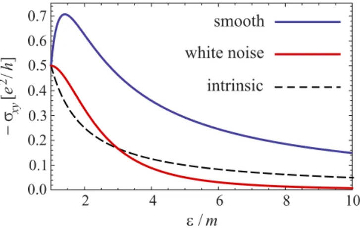
2m smooth white noise intrinsic
FIG. 2. The anomalous Hall conductivityσyx= −σxyin the units ofe2/2πh¯as a function of Fermi energy,ε > m, above the gap. The lower (red) solid line illustrates the result of Eq. (48) for the white- noise disorderα(φ)=α0. The upper (blue) solid line corresponds to the result of Eq. (53) for the case of smooth disorder defined in Eq. (49b). Dashed line refers to the intrinsic contribution which is given byσxyintin Eq. (28) in the absence of disorder.
result for the NCA contributionσxyncwas obtained in Ref. [37], while the full anomalous Hall conductivityσxyin the leading order with respect to disorder strength has been computed for the first time in Ref. [30].
The white-noise disorderα(φ)=α0 is characterized by a single Fourier componentα0in Eq. (3). In this case, the NCA contribution of Ref. [37] is readily reproduced from Eq. (27) as
σxync= −e2 2π
4εm(ε2+m2)
(ε2+3m2)2 , (46) which is manifestly independent of the white-noise disorder strength α0 and decays as m/ε for εm. The additional contribution of the crossed X and diagrams defined by Eq. (43) reads
σxyX+ = e2 2π
4εm(ε2−m2)
(ε2+3m2)2 , (47) in agreement with Ref. [30]. Note that this contribution is similarly independent ofα0and decays asm/ε. One can also see thatσxyX+andσxynchave opposite signs leading to a reduced value [30] of the totalσxywith respect to the NCA result [37].
Indeed, the total Hall conductivity σwhite noise
xy = −e2
2π
8εm3
(ε2+3m2)2, (48) demonstrates a much faster decay (m/ε)3 in the metal limit εm. We will see that such an essential cancellation of the AHE at large energies is a special property of the white-noise disorder.
The anomalous Hall conductivity of Eq. (48) is illustrated in Fig. 2 for the case of short-range white-noise disorder, α(φ)=α0, by red (lowest solid) line. The intrinsic contribution σxyint= −e2m/4π εfrom Eq. (28), which would remain in the absence of disorder, is plotted in the same figure with the dashed line. Note that none of the curves actually depend on the disorder parameterα0. Forεm, the extrinsic and
intrinsic contributions almost cancel each other such that the corresponding σxy decays as (m/ε)3 instead of the inverse linear decay of intrinsicσxyintand extrinsicσxyextcontributions.
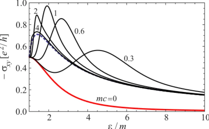
The monotonous decay of σxy with energy ε, as well as the cancellation of the leading terms∝m/εbetween intrinsic and extrinsic contributions at high energies, are not generic features of a weakly disordered system, but rather a specific property of the short range white-noise disorder corresponding to isotropic correlator α(φ)=α0. Despiteσxy is insensitive to the overall strength of a (weak) disorder, i.e., it does not change when all harmonicsαnare simultaneously multiplied by an arbitrary numerical factor, it turns out to be very sensitive to the correlation properties of disorder in general, i.e., to the relative magnitudeof the angular harmonicsαn. This interesting property is not at all limited to the model of massive Dirac fermions considered in the present paper, but extends to any metal system where the AHE conductivity is subleading (with respect to disorder strength) as compared to the longitudinal one.
B. Smooth disorder
The limit of smooth disorder is characterized by small angle scattering with the functionα(φ) peaked aroundφ=0.
A natural model for such long-range correlated disorder is provided by the angular diffusion. The latter is specified by the angular harmonics in Eq. (3) of the following form:
αn=a−bn2, (49a)
a = dφ
2πα(φ), b=1 2
dφ
2πφ2α(φ)a, (49b) where the parameter a represents the forward scattering probability, while the parameterbis the diffusion coefficient in the space of momentum angles (we remind that the absolute value of the momentum is pinned to the Fermi surface).
One observes immediately that the forward-scattering parametera does enter neither the diagonal nor anomalous Hall conductivity. Indeed, the transport rate of Eq. (20), which definesσxxin Eq. (22), and both the NCA (27) and the crossed (43) contributions to the Hall conductivity in Eq. (44) depend only on the angular harmonics differences βn=αn−αn−1 withn1. Consequently, the forward scattering parametera is manifestly canceling out from all transport quantities. We stress, however, that the forward scattering enters explicitly to the quantum scattering rateτ−1=π(a ε−b p20/ε) as is readily seen from Eq. (11). This rate describes the decay of a given quantum state, which remains finite even in the limit b→0.
From Eqs. (20)–(22), we obtain the longitudinal conduc- tivityσxx ∝τtr=1/2π εb, which is inversely proportional to the diffusion parameterb. In contrast, the Hall conductivity σxy=O(αn0) is again a function of ε/monly and does not depend explicitly on disorder strength. Upon substitution of Eq. (49b) into Eq. (27), we obtain the NCA contribution in the form
σxync= −e2 2π
m ε − m3
2ε3
, (50)
![FIG. 1. Diagrams representing the leading contributions to the longitudinal conductivity σ xx = O (α −1 n ) (a) and the anomalous Hall conductivity σ xy = O (α 0 n ) [(b), (c), and (d)]](https://thumb-eu.123doks.com/thumbv2/1library_info/3942658.1533606/4.911.77.443.103.352/diagrams-representing-leading-contributions-longitudinal-conductivity-anomalous-conductivity.webp)