Team decision-making

(1)

Team decision-making

Martin Kocher

University of Munich

Course in Behavioral and Experimental

Economics

(2)

(c) M. Kocher and M. Sutter 2

Motivation

The ‘decision maker’ is usually modeled as an individual in economics, but many real-life decisions are team

decisions.

Think of (hiring) committees, executive boards, advisory boards, households, etc. deciding on job offers,

monetary policy, corporate business strategy, judicial questions, household savings ...

(3)

Motivation

• (Social) Psychology has long been interested in

comparing team decisions to individual decisions, but has provided rather mixed results (see Levine and

Moreland, 1998, in Handbook of Social Psychology).

• Team decision making has captured vivid interest in (behavioral) economics only in recent years (see the top ten open research questions of Camerer, 2003).

(4)

Some open questions

• Do teams make different decisions than individuals – and under which circumstances?

• Which decision maker is more ‘successful‘ in strategic interaction?

• What drives team decision-making?

(5)

Preview

- Bargaining and social preferences

+ Ultimatum game (Bornstein and Yaniv, 1998) + Centipede game (Bornstein et al., 2004)

- Price competition (Bornstein and Gneezy, 2002) - Signaling game (Cooper and Kagel, 2005)

- Guessing game (Kocher and Sutter, 2005)

- Coordination games (Feri, Irlenbusch and Sutter, 2010)

(6)

Bargaining

• Bargaining often takes place between teams (think of negotiations on company mergers, peace treaties,

…).

• The seminal paper that studies differences between individuals and teams in simple bargaining games is by Bornstein and Yaniv (1998).

• They use the ultimatum game by Güth et al. (1982).

(7)

The ultimatum game

• 2 players (proposer and responder) bargain how to split an amount X.

• 2 stages:

• Proposer offers s to responder, keeping X – s.

• Responder has 2 options

– Responder accepts the offer s:

payoffs Proposer: X-s

Responder: s

– Responder rejects the offer s:

payoffs Both receive zero (0)

(8)

They conduct two treatments of the ultimatum game – Individuals: Both proposer and responder are

individuals.

– Teams: Teams of three subjects each are either in the role of proposer or responder.

Per-capita incentives constant.

Team decision made after 10 minutes of discussion.

One-shot game.

Control-treatment with double-blind procedure.

Bornstein and Yaniv (1998) – Design

(9)

Three main hypotheses

1. Teams are more competitive (discontinuity-effect of Insko and Schopler, 1992).

 Lower offers and higher rejection rates of teams.

2. Teams make less mistakes and are, thus, more rational.

 Lower offers, but no difference in rejection rates.

3. Teams are more normative (a bit vague in the paper).

 Identical offers, but lower rejection rates.

Bornstein and Yaniv (1998) - Hypotheses

(10)

Bornstein and Yaniv (1998) – Results

Single-blind

Double-blind

• Teams offer significantly less. There are almost no rejections.  Teams are “more rational”.

• There is no significant difference between single- and double-blind.

(11)

Additional evidence on bargaining

• Cason and Mui (1997): Dictator game – Teams give more.

• Luhan et al. (forthcoming): Dictator game – Teams give less.

• Kocher and Sutter (2007): Gift exchange game – Teams choose higher wages, but less effort.

• Cox (2002) and Kugler et al. (2007): Trust game – Teams give less and give back less.

(12)

They test team vs. individual behavior in two versions of the centipede game, where two players alternate in moves.

The increasing-sum centipede game

Another test on “rationality” – Bornstein,

Kugler and Ziegelmeyer (2004)

(13)

The constant-sum centipede game

Bornstein et al. (2004)

(14)

Two treatments

– Individuals: Both players are individuals.

– Teams: Both players are teams of three subjects.

Constant per-capita incentives, and free-form communication.

One-shot game.

Standard equilibrium is to “Take” at first node.

Bornstein et al. (2004) – Design

(15)

Bornstein et al. (2004) – Results

∅ node 5.22

∅ node 4.44

2.56 2.00

p < 0.01

p < 0.05

(16)

Social psychology offers some explanations for the earlier exit of the game by teams (called “groups” in Bornstein et al., 2004).

Among them are

- Stronger concerns for own payoffs in teams - Less identifiability in teams

- More competitiveness of teams because they expect other teams to be more competitive.

Bornstein et al. (2004) – Results

(17)

The previous papers – and the final ones – compared

individual and team decision-making where the payoffs in teams were identical across members.

Yet, it seems natural to ask what happens to team decisions if a team’s decision may yield different payoffs for its

members, hence when conflict is possible.

Think of two conglomerates of firms competing against each other (in building a new airplane, for instance). Then there might be internal conflicts within a conglomerate.

Team decision-making from a different

angle – Bornstein and Gneezy (2002)

(18)

• They study duopolistic price competition.

• Teams consist of 3 members (10 cohorts of 12 subjects).

• Team composition changes in each of 100 rounds.

• Two teams compete in prices.

• Each team member submits an integer bid from {2, …, 25}.

• The team with the smaller sum of bids wins the game and earns its sum of bids. The losing team earns nothing.

• Two treatments

+ Non-cooperative. Each member receives his bid.

+ Cooperative. Equal division of sum of bids.

Bornstein and Gneezy (2002) – Design

(19)

Cooperative team decisions lead to lower bids  less free- riding on other team members. Internal conflicts in non-

cooperative condition have impact on competition.

Bornstein and Gneezy (2002) – Results

Mean bid per round

(20)

Consider a situation where a monopolist faces a possible entrant. The entrant does not know the monopolist’s cost type (either high or low), but can only observe the

monopolist’s choice of quantities. What shall the monopolist do? Which signal should he send, and how should the

possible entrant react?

Such a situation has been modeled as an “entry limit pricing game” by Milgrom and Roberts (1982).

Cooper and Kagel (2005) have observed individual and team play in such a game.

Signaling games – Strategic play

(21)

Strategic play in such a game takes place through limit pricing, which means to choose larger quantities than would prevail in the absence of asymmetric information.

Cooper and Kagel were interested in testing how the “type of decision-maker” affects strategic play in such games.

Signaling games – Strategic play

(22)

• Monopolist (M)

– Type: high cost (MH) or low cost (ML) with equal probability

– Chooses output level

• Possible entrant (E) – Knows probability of

ML or MH

– Receives signal

through chosen output level

– Enters the market or not (IN or OUT)

Basic game

(23)

Monopolist‘s payoffs

• Monopolists prefer OUT over IN.

• MLs prefer generally higher outputs than MHs. (Myopic best choice would be 4 for ML, and 2 for MH.)

• “6” and “7” are dominated choices for MH. Thus, choosing “6”

may distinguish an ML from an MH.

(24)

Entrant‘s payoffs

Entrants have either high costs (top) or low costs (bottom). Costs are exogenously determined.

(25)

For high-cost entrants (the expected value of OUT is larger than the expected value of IN) there are both pooling and separating equilibria.

• In the pooling equilibria both types of monopolists choose any quantity from “1” to “5”, and the entrant stays OUT.

• In the separating equilibria the MLs choose “6”, and MHs choose “2”, since they cannot benefit from imitating an ML.

The entrant enters against MH, but stays out against ML.

For low-cost entrants (IN has higher expected value as OUT) only the separating equilibria from above remain.

Predictions for the game

(26)

They run three conditions - Only high-cost entrants.

- Only low-cost entrants.

- First high-cost entrants and then low-cost entrants (crossover-treatments to examine transfer learning).

All conditions are run both with - Individuals.

- Teams of two subjects who can communicate via chat. In case of no agreement on quantity within 3 minutes, one member is determined as “leader” who can decide.

Cooper and Kagel (2005) – Design

(27)

Hypothesis 1: There will be more strategic play of teams than of individuals.

Strategic play is defined as MHs choosing “3” to “5”, and

MLs choosing “5” to “7”. These levels are above the myopic best choice of “2” for MHs, and “4” of MLs.

Hypothesis 2: The level of strategic play of teams will meet or beat a truth-wins norm.

Let p (P) be the probability of an individual (team) playing strategically, then teams beat the truth wins-norm if

P ≥ 1 – (1 – p)².

Cooper and Kagel (2005) – Hypotheses

(28)

- Teams in the role of MH act a bit more strategically (p < 0.1 in cycle 1), but a truth wins norm is not reached.

High-cost entrants – Results

Proportion of strategic play of MHs.

Individuals Teams

Simulated teams

(29)

- Teams in the role of ML act significantly more often strategically (p < 0.05 in all cycles).

Low-cost entrants – Results

Proportion of strategic play of MLs.

Individuals Teams

Simulated teams

(30)

Monopolists start facing high-cost entrants (for 2 cycles, i.e. 24 periods, in inexperienced mode, and 1 cycle, i.e. 8 periods, in experienced mode).

Then there is a switch to low-cost entrants (for another 3 cycles, i.e. 24 periods).

This crossover treatment allows examining the transfer of knowledge acquired in a specific strategic situation to a similar one.

In particular, it allows to analyse whether teams are better in learning transfer. The answer is clearly “Yes” (contrary to the authors’ Hypothesis 3).

Cooper and Kagel (2005) –

The crossover treatments

(31)

- After the crossover, teams play much more strategically than individuals.

Crossover treatment – Results

Individuals Teams

Simulated teams

(32)

- After the crossover, teams play more strategically, but individuals less.  Better learning transfer in teams.

Transfer – Results

Teams after crossover (CO) Teams before CO

Individuals before CO

Individuals after CO

(33)

Analyzing the team dialogues (one of the novel parts of this paper for an economics audience!) reveals that strategic play and learning in the crossover-games depend critically on teams discussing how the strategic situation is viewed from the entrant’s perspective! Putting yourself in the shoes of the entrant reveals the possibility of pooling or separating equilibria.

(One note on limitation: It would be desirable to have access also to individuals’ stream of thinking to compare it to the team dialogues. However, …)

Some insights from the team dialogues

(34)

Team behavior in the guessing game

The guessing game

• N decision makers simultaneously choose a real number from the interval [0, 100].

• The winner is the decision maker whose number is closest to 2/3 of the average number.

• The game’s unique equilibrium is to choose zero.

(35)

Hypotheses

(based on information load theory; Chalos and Pickard, 1985)

1. Convergence to equilibrium

– Teams apply more steps of reasoning and pick lower numbers than individuals.

2. Relative performance

– Teams win more often than individuals when competing against each other (or are teams prone to the ‘curse of sophistication’?)

3. Influence of team size

– Larger teams should be more successful and converge faster to the equilibrium.

(36)

Kocher and Sutter (2005) – Design

Experiment 1

• Teams compete against teams (2 sessions; N = 35 in total)

• Individuals compete against individuals (2 sessions; N = 35 in total)

• 4 round

• Winner takes all (about 10 Euro)

• Feedback on all numbers.

• Paper and pen in large classes

(37)

Kocher and Sutter (2005) – Convergence to equilibrium

Median number

0 5 10 15 20 25 30 35

1 2 3 4

Round

Teams Individuals

Teams choose significantly lower numbers, except for round 1.

(38)

Relative performance in the

guessing game (Kocher, Strauß and Sutter 2006, GEB)

Part I:

N = 3 individuals play the game once  no feedback Self-selection phase:

Subjects can decide whether to play alone or in a team of three subjects (about 60% want to play in a team)

Part II:

2 individuals and 1 team paired for 4 rounds  regular feedback on others‘ numbers

(39)

Kocher et al. (2006) – Results

0 5 10 15 20 25 30 35 40 45

Part One Round 1 Round 2 Round 3 Round 4

Individuals Team members

Individual choices part I

Teams

Individuals

Team members choose significantly higher numbers in part I (as individuals), but significantly lower numbers in part II (as teams).

(40)

0 0.5 1 1.5 2 2.5 3 3.5 4 4.5

Round 1 Round 2 Round 3 Round 4

Average profits in euros

Individuals Teams

Kocher et al. (2006) – Results

Average profits in Euro

Individuals Teams

Teams earn significantly larger amounts

(41)

• Subjects select into teams because of the (ex post

correct!) expectation of earning higher profits in teams.

• Subjects’ main motive for individual decision-making is a preference for deciding alone, without the need for

compromise and discussion.

• Individual decision-makers correctly guess (after the

experiment) that teams won more money, however they indicate to be as happy with their role as team members do.

• Thus, subjects are willing to pay a price for their preference to decide alone.

Kocher et al. (2006) – Self-selection

(42)

• No study has ever considered more than two ‘sizes’

of decision makers.

• However, team size may affect (the quality of) decision making (see information load theory).

• 3 different decision makers interact for 4 rounds – 1 individual

– 1 team with 2 members – 1 team with 4 members

Sutter (2005, EL) – Influence of team size

(43)

(c) M. Kocher and M. Sutter 43 Average numbers

0 5 10 15 20 25 30 35 40 45

Individual 2 members 4 members

Sutter (2005) – Results

Larger teams choose smaller numbers (significant in all rounds)

(44)

(c) M. Kocher and M. Sutter 44 Absolute win frequency

0 2 4 6 8 10 12 14 16 18

number of wins

Individual 2 members 4 members

Sutter (2005) – Profits

Larger teams win more often.

(45)

Surprisingly, so far there have only been (experimental) studies that investigate the coordination behavior of

individuals, whereas the behavior of teams has not been examined (see the excellent survey of Devetag and

Ortmann, 2007).

However, team decision-making and coordination across teams is a widespread phenomenon. For instance, Knez and Simester (2001) illustrate in a very nice field study the need for coordination among teams at Continental Airlines to manage on-time departures and arrivals.

Teams in coordination games

(46)

Feri, Irlenbusch and Sutter (2010) – Design

- 2 weakest-link games (alias minimum-games) - 4 average-opinion games (alias median-games)

- 5 decision makers constitute a “group”: either 5 individuals or 5 teams á three subjects (chat communication)

- 20 periods with partner-matching

- Feedback: Minimum/Median in particular period - Computerized (Fischbacher, 2007)

- Average duration: 45-65 minutes

- Average payoff: 9€, plus 2.5€ show-up fee

(47)

The weakest-link game WL-GAME

Table 1: Payoffs in weakest-link game WL-GAME Smallest number chosen in your group

7 6 5 4 3 2 1

7 130 110 90 70 50 30 10

6 120 100 80 60 40 20

5 110 90 70 50 30

4 100 80 60 40

3 90 70 50

2 80 60

1 70

Your number

Payoff-dominance: “7” Risk-dominance: “1”

(48)

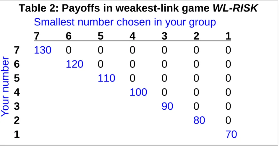
The weakest-link game WL-RISK

Table 2: Payoffs in weakest-link game WL-RISK Smallest number chosen in your group

7 6 5 4 3 2 1

7 130 0 0 0 0 0 0

6 120 0 0 0 0 0

5 110 0 0 0 0

4 100 0 0 0

3 90 0 0

2 80 0

1 70

Your number

(49)

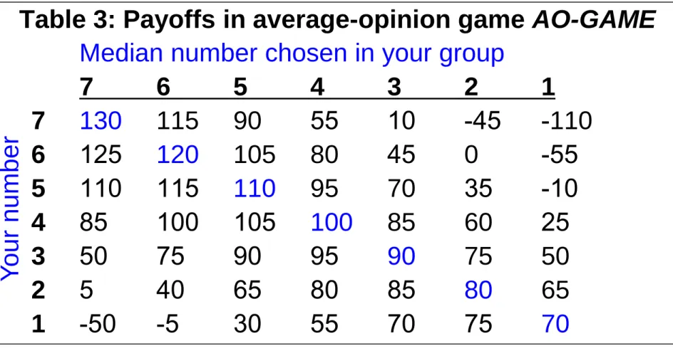
The average-opinion game AO-GAME

Table 3: Payoffs in average-opinion game AO-GAME Median number chosen in your group

7 6 5 4 3 2 1

7 130 115 90 55 10 -45 -110

6 125 120 105 80 45 0 -55

5 110 115 110 95 70 35 -10

4 85 100 105 100 85 60 25

3 50 75 90 95 90 75 50

2 5 40 65 80 85 80 65

1 -50 -5 30 55 70 75 70

Your number

(50)

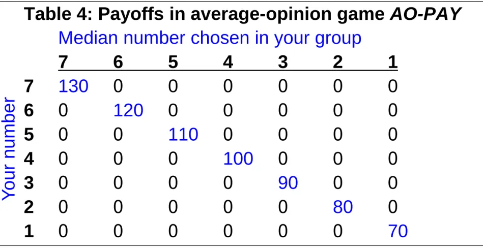
The average-opinion game AO-PAY

Table 4: Payoffs in average-opinion game AO-PAY Median number chosen in your group

7 6 5 4 3 2 1

7 130 0 0 0 0 0 0

6 0 120 0 0 0 0 0

5 0 0 110 0 0 0 0 4 0 0 0 100 0 0 0

3 0 0 0 0 90 0 0

2 0 0 0 0 0 80 0

1 0 0 0 0 0 0 70

Your number

Payoff-dominance: “7” Risk-dominance: n.a.

(51)

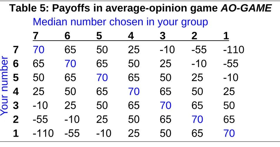
The average-opinion game AO-RISK

Table 5: Payoffs in average-opinion game AO-GAME Median number chosen in your group

7 6 5 4 3 2 1

7 70 65 50 25 -10 -55 -110 6 65 70 65 50 25 -10 -55

5 50 65 70 65 50 25 -10

4 25 50 65 70 65 50 25

3 -10 25 50 65 70 65 50

2 -55 -10 25 50 65 70 65

1 -110 -55 -10 25 50 65 70

Your number

Payoff-dominance: n.a. Risk-dominance: “4”

(52)

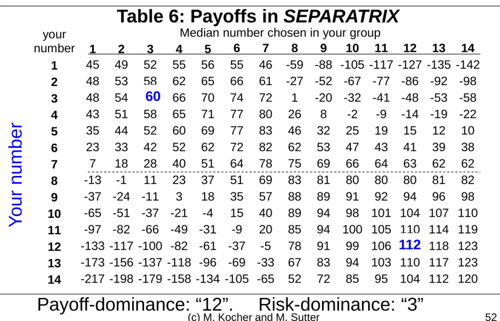
The average-opinion game SEPARATRIX

Your number

Payoff-dominance: “12”. Risk-dominance: “3”

Median number chosen in your group your

number 1 2 3 4 5 6 7 8 9 10 11 12 13 14 1 45 49 52 55 56 55 46 -59 -88 -105 -117 -127 -135 -142 2 48 53 58 62 65 66 61 -27 -52 -67 -77 -86 -92 -98 3 48 54 60 66 70 74 72 1 -20 -32 -41 -48 -53 -58 4 43 51 58 65 71 77 80 26 8 -2 -9 -14 -19 -22 5 35 44 52 60 69 77 83 46 32 25 19 15 12 10 6 23 33 42 52 62 72 82 62 53 47 43 41 39 38 7 7 18 28 40 51 64 78 75 69 66 64 63 62 62 8 -13 -1 11 23 37 51 69 83 81 80 80 80 81 82 9 -37 -24 -11 3 18 35 57 88 89 91 92 94 96 98 10 -65 -51 -37 -21 -4 15 40 89 94 98 101 104 107 110 11 -97 -82 -66 -49 -31 -9 20 85 94 100 105 110 114 119 12 -133 -117 -100 -82 -61 -37 -5 78 91 99 106 112 118 123 13 -173 -156 -137 -118 -96 -69 -33 67 83 94 103 110 117 123 14 -217 -198 -179 -158 -134 -105 -65 52 72 85 95 104 112 120

112 60

Table 6: Payoffs in SEPARATRIX

(53)

Experimental procedure

Experiments run in academic year 2006/07

- Weakest-link games at University of Cologne

- Average-opinion games at University of Innsbruck Participants # groups (N) Game Ind. Teams Ind. Teams

WL-GAME 90 135 18 9

WL-RISK 30 90 6 6

AO-GAME 30 90 6 6

AO-PAY 30 90 6 6

AO-RISK 30 90 6 6

SEPARATRIX 30 90 6 6

Σ = 825

(54)

Feri, Irlenbusch and Sutter (2010) – Results

Table 7: Average numbers in 1^st period and overall

1^st period All periods

Coordination game Individual Team Individual Team

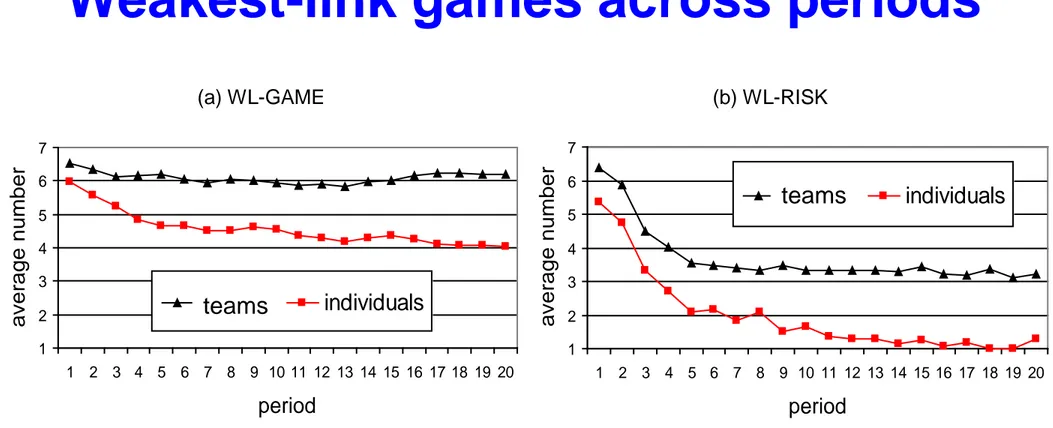
WL-GAME (Tab. 1) 5.98 <** 6.53 6.06 <* 6.56 WL-RISK (Tab. 2) 5.37 <*** 6.37 1.97 < 3.70

AO-GAME (Tab. 3) 5.67 < 6.17 6.57 <** 6.94

AO-PAY (Tab. 4) 5.33 <*** 6.43 6.04 <** 6.95

AO-RISK (Tab. 5) 4.43 ≈ 4.40 4.07 ≈ 4.03

SEPARATRIX (Tab. 6) 7.90 <*** 11.03 9.80 <** 12.63

Observations 1: Teams choose higher numbers.

Observations 2: Teams get significantly higher payoffs.

(except in AO-RISK where payoff-dominance does not apply)

(55)

Weakest-link games across periods

Figure 1: Average numbers chosen in the weakest-link games

(a) WL-GAME (b) WL-RISK

1 2 3 4 5 6 7

1 2 3 4 5 6 7 8 9 10 11 12 13 14 15 16 17 18 19 20

period

average number

groups individuals

1 2 3 4 5 6 7

1 2 3 4 5 6 7 8 9 10 11 12 13 14 15 16 17 18 19 20

period

average number

groups individuals

teams

(56)

Average-opinion games across periods

(a) AO-GAME (b) AO-PAY

1 2 3 4 5 6 7

1 2 3 4 5 6 7 8 9 10 11 12 13 14 15 16 17 18 19 20

period

average number

groups individuals

1 2 3 4 5 6 7 8 9 10 11 12 13 14

1 2 3 4 5 6 7 8 9 10 11 12 13 14 15 16 17 18 19 20

period

average number

groups individuals

1 2 3 4 5 6 7

1 2 3 4 5 6 7 8 9 10 11 12 13 14 15 16 17 18 19 20

period

average number

groups individuals

1 2 3 4 5 6 7

1 2 3 4 5 6 7 8 9 10 11 12 13 14 15 16 17 18 19 20

period

average number

groups individuals

(c) AO-RISK (d) SEPARATRIX

teams

(57)

Miscoordination and adjustments across periods

Observation 3: Teams are more successful in avoiding miscoordination and settle quicker in an equilibrium.

Table 8: Coordination and adjustment

Miscoordination Adjustment

Coordination game Individual Team Individual Team

WL-GAME (Tab. 1) 0.65 >** 0.30 0.60 >* 0.29 WL-RISK (Tab. 2) 0.39 >* 0.29 0.53 >** 0.21 AO-GAME (Tab. 3) 0.14 >*** 0.06 0.09 >** 0.03

AO-PAY (Tab. 4) 0.25 >** 0.03 0.34 >* 0.02

AO-RISK (Tab. 5) 0.12 > 0.04 0.10 > 0.01

SEPARATRIX (Tab. 6) 0.84 >*** 0.51 0.98 >*** 0.56

(58)

What drives team behavior?

In psychology, team decision-making is often related to a so-called “truth wins”-norm (in demonstrable tasks). I.e., if one team member advocates the “true” solution, then the others are easily convinced for that.

We examine whether the observed team behavior can be explained by a

- “payoff-dominance wins”-norm, or a - “risk-dominance wins”-norm.

(59)

A simulation approach

We take the observed individual data (in a given game and period) and randomly assign three individuals into a

team. If one of the individuals has chosen the payoff-

dominant (or the risk-dominant) action, then we assume that the team would have chosen that action as well.

We run 100,000 simulations (per game and period) and calculate from that the expected frequency of playing either the payoff-dominant or the risk-dominant action.

We also calculate confidence-intervals to check whether the actually observed team-decisions lie within these

intervals.

(60)

Simulation results on payoff-dominance in weakest-link games

0 0.2 0.4 0.6 0.8 1

1 2 3 4 5 6 7 8 9 10 11 12 13 14 15 16 17 18 19 20 period

proportion of payoff dominant play

simulated groups individuals groups

0 0.2 0.4 0.6 0.8 1

1 2 3 4 5 6 7 8 9 10 11 12 13 14 15 16 17 18 19 20 period

proportion of payoff dominant play simulated groups individuals groups

(a) WL-Game (b) WL-RISK

Rel. freq. payoff-dominant choice

Individuals Teams Simulated teams (with confidence intervals)

(61)

Simulation results on payoff-

dominance in average-opinion games

0 0.2 0.4 0.6 0.8 1

1 2 3 4 5 6 7 8 9 10 11 12 13 14 15 16 17 18 19 20 period

0 0.2 0.4 0.6 0.8 1

1 2 3 4 5 6 7 8 9 10 11 12 13 14 15 16 17 18 19 20 period

0 0.2 0.4 0.6 0.8 1

1 2 3 4 5 6 7 8 9 10 11 12 13 14 15 16 17 18 19 20 period

(a) AO-GAME (b) AO-PAY

(c) SEPARATRIX

Observation 4: The more efficient coordination in teams can be explained by a “payoff-dominance wins”-norm.

(62)

Simulation results on risk- dominance

0 0.2 0.4 0.6 0.8 1

1 2 3 4 5 6 7 8 9 10 11 12 13 14 15 16 17 18 19 20 period

proportion of risk dominant play

0 0.2 0.4 0.6 0.8 1

1 2 3 4 5 6 7 8 9 10 11 12 13 14 15 16 17 18 19 20 period

proportion of risk dominant play

(a) WL-GAME (b) WL-RISK

0 0.2 0.4 0.6 0.8 1

1 2 3 4 5 6 7 8 9 10 11 12 13 14 15 16 17 18 19 20 period

proportion of risk-dominant play

(c) AO-RISK

Observation 5: Teams are significantly less likely to follow a “risk- dominance wins”-norm (if payoff-dominance applies).

(63)

Could our findings have been expected?

Relation to team decision-literature

1) Teams have been found to be closer to standard game theoretic predictions (in bargaining games, signaling games, …, see Kocher and Sutter, 2005, for a review).

 However, this regularity does not solve the equilibrium selection problem.

2) Teams care more for own payoffs (and exhibit less social preferences, see Bornstein and Yaniv, 1998).

 This might explain why payoff-dominance is relatively more important for teams.

3) Teams are not per se more risk-averse or risk-loving (see Shupp and Williams, 2007).

 This might explain the results in AO-RISK.