Research Collection
Report
System Analysis of Mesoscale and Microscale Urban Climate Simulation Workflows
Author(s):
Li, Shiying; Aydt, Heiko Publication Date:
2020-08
Permanent Link:
https://doi.org/10.3929/ethz-b-000432258
Rights / License:
In Copyright - Non-Commercial Use Permitted
DELIVERABLE TECHNICAL REPORT
Version 04/08/2020
D3.1 – System Analysis of Mesoscale and Microscale Urban Climate Simulation Workflows
Project ID NRF2019VSG-UCD-001
Project Title Cooling Singapore 1.5:
Virtual Singapore Urban Climate Design
Deliverable ID D3.1 – System Analysis of Mesoscale and
Microscale Urban Climate Simulation Workflows
Authors Shiying Li, Heiko Aydt
DOI (ETH Collection)
Date of Report 04/08/2020
Version Date Modifications Reviewed by
1 11/06/2020 Version 1 Prof. Dr. Leslie Norford, Dr. Jimeno Fonseca
Abstract
The Cooling Singapore project studies the urban climate of Singapore and, in particular, evaluates measures to mitigate urban heat. For this purpose, Cooling Singapore utilises a variety of tools for modelling, simulation, data processing and analysis. Some of these tools are off-the-shelf software (e.g., MATLAB, ANSYS Fluent), while others are third-party open-source software modified to meet the needs of the project (e.g., WRF), or software that has been developed in-house specifically for the purpose of the project. The resulting ecosystem of tools is thus highly diverse, requiring a diverse set of skills and operating environments in order to perform integrated studies across multiple domains. At the moment, such integrated studies are carried out in a collaborative manner involving the contributions from various researchers.
The ability to carry out integrated what-if scenario analysis is important to investigate the potential impact of mitigation measures on the urban climate. This ability is not only important for researchers but also for practitioners, such as urban planning authorities for example. Manual workflow execution, involving the contributions of several researchers, represents a significant constraint. Not only is this process time-consuming, it is also prone to human error. A better approach would be to clearly specify the individual steps needed to carry out a particular what-if scenario analysis and automate (as far as possible) the entire process. This would not only reduce the amount of manual work (thus freeing researchers’ time to focus on other things) but also vastly improve the reproducibility of results and reduce the likelihood of human error.
The first steps towards automated workflow execution are to analyse the workflows to better understand the various steps that are needed in order to carry out integrated studies and what-if scenario analyses.
This document represents a systematic analysis of the primary workflows and their principal components in the context of the Cooling Singapore project. In particular, this document provides an overview of all principal components, as well as their input and output data. The information provided in this document is not meant to be a detailed documentation for each of the various model components.
Instead, it is a system-level analysis that focuses on the flow of data from one model to another. It should also be noted that the information provided here is valid as of the time of writing. However, as the project evolves, so will the workflows and the components of the system.
Table of Content
Abstract ... 2
1 Introduction ... 4
1.1 Background ... 4
1.2 Objectives ... 5
1.3 Methodology ... 5
1.4 Limitations ... 7
2 Workflows and Principal Components ... 8
2.1 Mesoscale Urban Climate Model ... 11
2.2 Microscale Urban Climate Model ... 18
2.3 Mesoscale Traffic Model ... 30
2.4 Building Energy Model ... 37
2.5 Power Plant Dispatch Model ... 44
2.6 Industry Heat Model ... 46
2.7 Microscale Traffic Model ... 49
2.8 Weather Types Clustering ... 52
3 Concluding Remarks ... 55
List of Acronyms ... 56
References ... 58
Annex A – General Mesoscale Workflow ... 60
Annex B – General Microscale Workflow ... 61
1 Introduction
1.1 Background
The Cooling Singapore project utilises a variety of tools for modelling, simulations, data processing and analysis. Some of these tools are off-the-shelf software (e.g., MATLAB, ANSYS Fluent), while others are third-party open-source software (e.g., WRF) which are modified to meet the needs of the project.
In addition, the Cooling Singapore project also uses software which has either been developed by a participating project partner (e.g., CityMoS, CEA) or as part of the Cooling Singapore project itself (e.g., Power Plant Dispatch Model). The resulting tool ecosystem is thus highly diverse. Operational requirements are just as diverse. Some tools require very specific execution environments (e.g., high- performance computing environments) while others can be operated in standard desktop/laptop environments.
Most researchers are specialised in using a small set of tools for a specific purpose. For example, while one researcher specialises in using urban climate models to perform urban climate simulations, he/she is not an expert for building energy simulation which, in turn, is the domain of someone else. In addition to such domain-specific research activities, Cooling Singapore also concerns itself with integrated studies and what-if scenario analyses. Integrated studies span multiple domains in a highly- interdependent manner. At the moment, such integrated studies are carried out in a collaborative manner. Integrity and reproducibility, as well as analysis and interpretation of results, have to be manually ensured.
The ability to carry out integrated what-if scenario analysis is important to investigate the potential impact of mitigation measures on the urban climate. This ability is not only important for researchers but also for practitioners, such as urban planning authorities for example. A manual workflow, involving the contribution of several researchers, represents a significant constraint. It is not only time-consuming, but it is also prone to human error. A better approach would be to clearly specify the individual steps needed to carry out a particular what-if scenario analysis and automate (so as far as possible) the entire process. This would not only reduce the amount of manual work (thus freeing researchers’ time to focus on other things) but also vastly improve the reproducibility of results and reduce the likelihood of human error.
The first steps towards automated workflow execution are to analyse the workflows to better understand the various steps that are needed in order to carry out integrated studies and what-if scenario analyses.
The second step is to develop the necessary infrastructure for automating these steps and to combine
them into automated workflows. This document represents a systematic analysis of the primary workflows and their principal components in the context of Cooling Singapore.
1.2 Objectives
One important aspect of this work is to clearly identify and describe the individual steps, their inputs and outputs as well as how the output of one model is used as input for another model as part of the larger workflow. The result of this work is an overview of (1) the principal components needed to conduct integrated urban climate what-if scenario analysis; as well as (2) the important data objects consumed and produced by these components. This report represents a system analysis and the foundation for implementing the necessary infrastructure for automated workflow execution.
1.3 Methodology
Workflow analysis is the process of breaking down a complex process into its components and identifying the flow of information or data between them. This allows us to gain more insights into the individual components and how they interact with each other. Analysis of the workflows in the Cooling Singapore project has been done primarily by interviewing the individual researchers to better understand what they do, what tools they are using for modelling, what input data is needed by their models to simulate a scenario and what output data are ultimately generated by the simulations.
Data flow diagrams1 aid in the analysis process. This kind of diagram provides information about the inputs and outputs of the various entities in a system. In the context of the workflow analysis, we will use the term workflow diagram to refer to the data flow diagrams featuring the following three basic elements: processor, function and data object. Figure 1.3.1 shows a generic example of these elements. They are further explained in the remainder of this section.
1 Data flow diagram: see (Ibrahim, 2010) and (Li and Chen, 2009, page 85).
Figure 1.3.1: Basic elements in a workflow diagram.
Processor
A processor is a complex process which processes input data and produces output data. It typically requires significant computational resources, memory, or storage to perform. Due to its complexity, a processor is expected to require a longer period of time to generate a response to requests. Execution of a processor is thus assumed to be asynchronous, i.e., the requesting entity will not wait for a processor to respond immediately. Instead, it will check in regular intervals if the processor has finished and if the processor’s response is now available. Examples for processors include computationally heavy urban climate simulations using WRF and computational fluid dynamics simulations using Ansys Fluent. In the workflow diagram, a processor is indicated by a rectangular box with double vertical edges such as the one illustrated in Figure 1.3.2.
Figure 1.3.2: Processor element as used in a workflow diagram.
Function
A function is similar to a processor in the sense that it processes input and generates output just as a processor. However, it has only limited computational requirements and is expected to require only a relatively short and limited amount of time to generate a response to requests. Execution of a function is thus assumed to be synchronous, i.e., the requesting entity will wait for the function to respond. It is commonly found in the data pre- and post-processing stages. In the workflow diagram, a function is indicated by a rectangular box (without double vertical edges) such as the one illustrated in Figure 1.3.3.
Figure 1.3.3: Function element as used in a workflow diagram.
Data Object
A data object is a well-defined and well-structured representation of the data that is used as input and generated as output by processors and functions. Data objects may come in any kind of format (e.g., JSON, CSV) and may be small (e.g., a few bytes) or large (e.g., many gigabytes). We assume data objects to come in the form of files (either used as input for or output of processors and functions) or streams (i.e., data that is being sent to or received from processors and functions). In-memory data objects would be expected to be made accessible either as files or streams. However, these are implementation-specific aspects which we are not further concerned with as part of the workflow analysis. Instead, we will focus on the nature of the content they entail. In the workflow diagram, a data object is indicated by a parallelogram such as the one illustrated in Figure 1.3.4.
Figure 1.3.4: Data object element as used in a workflow diagram.
1.4 Limitations
The findings presented in this document represent our understanding of the various workflows at the time of writing. As new use cases are emerging and existing use cases change, so do their corresponding workflows. At the time of writing, the workflows as well as details of their principal components are not fully defined yet. Nevertheless, the findings of our analyses provide a good overview of the complexity involved in carrying out integrated studies and provide sufficient information in order to proceed with the second step towards workflow automation, i.e., infrastructure development.
2 Workflows and Principal Components
Cooling Singapore utilises a number of models and tools for studying what-if scenarios concerned with the Urban Heat Island (UHI) and Outdoor Thermal Comfort (OTC) in Singapore. The same models and tools are also used to assess strategies to mitigate urban heat. Depending on the nature of the analysis, the exact workflow and selection of models and tools may vary. Automated workflow execution requires the execution of a number of models in a specific sequence. For this purpose, a workflow controller is needed that manages the execution of a workflow, i.e., triggering the various model components as well as managing the various data objects that are needed in the process. Conceptually, the overall system consists of three areas (as illustrated in Figure 2.0.1): parameters for defining what-if scenarios, a federation of models that carries out the workflow, and applications for decision support.
Figure 2.0.1: Conceptual overview of the three areas: parameters for what-if scenarios, federation of models, and decision support applications. Workflows involve the execution of a series of model components that use input data, provided by a given what-if scenario, and produce intermediate data which is used as input for other model components that are part of the workflow. Model components may be compositions of other components. The output of a workflow is ultimately used for analysis and decision support.
In Cooling Singapore, we generally distinguish between meso- and microscale workflows. While the former is used for city-wide studies, typically concerned with the UHI, the latter is used for neighbourhood and district-wide studies, typically concerned with OTC. Although the exact models and
tools used by the various workflows are different, they have in common that there are a number of models that estimate anthropogenic heat emissions by relevant sources, such as industry, building cooling systems and transport, whose simulation outputs are ultimately used as input for an urban climate model. These urban climate models use additional information about land-use (mesoscale) and information about geometry and materials used (microscale), as well as the information about anthropogenic heat emissions provided by the other models, to estimate climatic variables (e.g., air temperature, humidity, wind flow) in the area of interest.
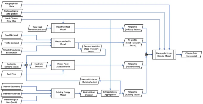
The general mesoscale workflow is illustrated in Figure 2.0.2. Anthropogenic Heat (AH) Profiles, generated by multiple anthropogenic heat emission models (industrial heat dispatch model, road transport, power plant dispatch model, building energy model) are used as input for the mesoscale urban climate model which produces mesoscale climate data. Evaluating a scenario of interest is done by using input data objects that sufficiently reflect the nature of the scenario.
Figure 2.0.2: General mesoscale workflow (see Annex A for full-page diagram).
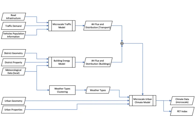
The general microscale workflow is illustrated in Figure 2.0.3. Similar to the mesoscale workflow, the microscale workflow consists of a number of models to estimate anthropogenic heat emissions (agent- based traffic model and building energy model) which is used as input for the urban climate model. In addition, the microscale urban climate model also takes meteorological data into consideration that reflects specific weather types as well as information about the urban geometry and properties of the area of interest.
Figure 2.0.3: General microscale workflow (see Annex B for full-page diagram).
In general, both workflows can be used to evaluate what-if scenarios. This is done by providing necessary input data when executing the workflows. For example, on the mesoscale, studying the impact of switching to all-electric vehicles can be done by using corresponding input data for vehicle population information. On the microscale, how well different urban geometries can mitigate heat can be studied using the microscale workflow with corresponding information that reflect different urban design scenarios. Furthermore, different model implementations can be used to reflect a particular scenario. For example, studying the impact of district cooling can be done by using a corresponding implementation of the 'building energy model’.
The remainder of Section 2 will provide further details about the principal components of the model federation that are needed for workflow execution.
2.1 Mesoscale Urban Climate Model
Urbanisation impacts the local weather and is responsible for the Urban Heat Island (UHI) effect, which is characterised by warmer temperatures in city areas compared to surrounding rural areas. A mesoscale urban climate model is used to study the city-wide UHI effect and climate development in different urban scenarios. The principal inputs and output of this component are illustrated in Figure 2.1.1.
Figure 2.1.1: Principal inputs and output of the mesoscale urban climate model component.
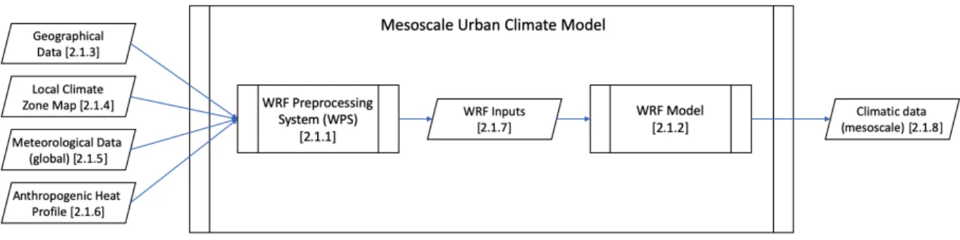
Cooling Singapore uses the Weather Research and Forecasting (WRF) model as its mesoscale urban climate model component in the mesoscale workflow. Figure 2.1.2 shows the two main components of WRF-related modelling and processing: the WRF Preprocessing System (WPS) and the actual WRF model, which will be explained in Section 2.1.1 and 2.1.2, respectively.
Figure 2.1.2: WPS and WRF components used as part of the mesoscale urban climate model.
WRF Preprocessing System (WPS)
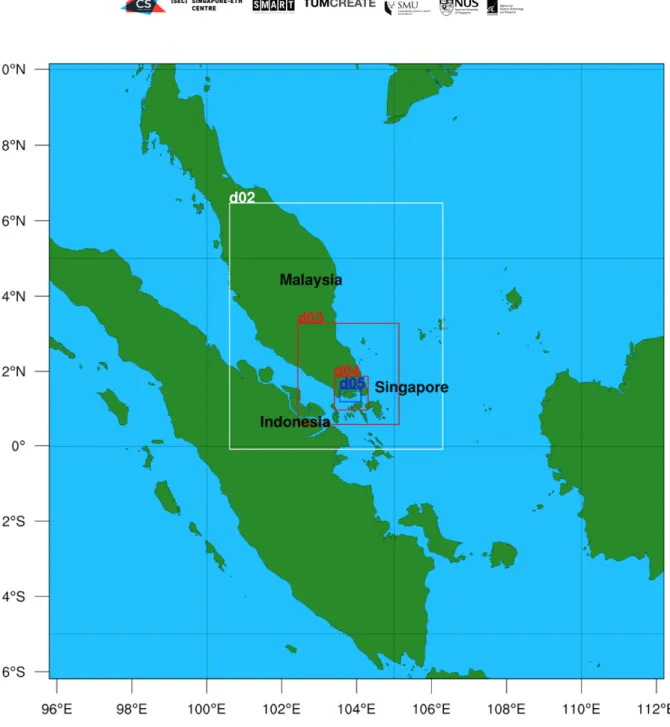
WRF Preprocessing System (WPS) illustrated in Figure 2.1.2 is a pre-processing processor that prepares the input data to the WRF model for real-data simulations. It consists of the initial WPS with a set of three programs (‘geogrid’, ‘ungrib’ and ‘metgrid’) and the WRF initialisation program ‘real’. The pre-processing processor is responsible for defining the simulation domain, extracting terrestrial and meteorological data from a global dataset, and interpolating the extracted data horizontally and vertically into the simulation domain. The WRF model used in Cooling Singapore has been configured with five simulation domains as illustrated in Figure 2.1.3, whereby the region of interest is the fifth domain containing the island of Singapore. As initial WPS completes the two-dimensional interpolation of input data, the WRF initialisation program ‘real’ will then interpolate the two-dimensional data vertically. The interpolated three-dimensional data (WRF inputs - see Section 2.1.7) provides the initial boundary conditions for the WRF model.
Weather Research and Forecasting (WRF) Model
The Weather Research and Forecasting (WRF) Model is a numerical urban climate model used to simulate the atmospheric development over an urban area and to study the interaction between urbanisation and the atmosphere in horizontal dimensions ranging from several hundred metres to hundreds of kilometres. It is mainly used for atmospheric research and operational forecasting applications. The WRF model can produce simulations based on actual atmospheric conditions (i.e., from observations) or idealised conditions (MMM, 2019-b). In Cooling Singapore, we simulate based on actual atmospheric conditions using the Advanced Research WRF dynamics core (WRF-ARW) and multi-layer urban canopy Building Effect Parameterization (BEP) and Building Energy Modelling (BEM)2. The BEP and BEM model are part of the urban canopy model and provide an estimation of energy consumption of buildings in the urban area. Modifications to the original WRF v3.8.1 source code have been made to support Local Climate Zones (Stewart and Oke, 2012) and allow for the integration of the various anthropogenic heat sources used by Cooling Singapore (see Figure 2.0.2).
2 BEP: Building Effect Parameterisation (Martilli et al., 2002) BEM: Building Energy Modelling (Salamanca and Martilli, 2010)
Figure 2.1.3: WRF model configuration with five domains. The whole illustration corresponds to Domain 1 (d01), whereby the Domain 5 (d05) is the region of interest for Cooling Singapore. (Source: Mughal et al., 2019)
The remainder of this section describes the principal inputs and output for the mesoscale urban climate model component and the WRF-related internal data objects.
Geographical Data
The geographical data is a static data set which contains time-invariant terrestrial data in various spatial resolutions. It contains static information about land use/land cover and its utilisation, such as soil types,
terrain height, monthly vegetation fraction land use categories and more. For more information refer to (Mughal et al., 2019) and the WRF V3 User’s Guide3. The data consists of two parts: the mandatory global terrestrial data set and an additional dataset, consisting of region-specific land surface information. The data is stored and distributed in the geogrid binary format that can be visualised and edited using GIS software. The complete, uncompressed global dataset can be up to 50 Gigabytes and is accessible via the WRF download page4.
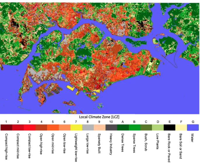
Local Climate Zone Map
The concept of the Local Climate Zone (LCZ) classification, as introduced by (Stewart and Oke, 2012), was developed to study the UHI phenomenon. The LCZ classification was primarily developed to describe the impact of land-use features on the near-surface local climate and the UHI. The scheme consists of 17 basic types which were characterised by different properties of the surface structure and the surface cover. LCZ maps are created using GIS software and stored as images in GeoTIFF format (a TIFF image file with embedded georeferencing information). Before this image can be processed by WPS, it has to be converted into the geogrid binary format.
Cooling Singapore developed an LCZ map for Singapore by adopting the World Urban Database and Access Portal Tools (WUDAPT) methodology based on satellite remote sensing imageries and building height data (Mughal et al., 2019). See Figure 2.1.4 for an illustration of the LCZ map that is created based on the cloud-free satellite images from the year 2015 to 2017. This LCZ map is used to represent present-day Singapore. It contains land surface information of Singapore in a 30 m spatial resolution (which is the same resolution as the satellite images used). The LCZ map provides additional land surface information (e.g., Land Use/Land Cover) that increases the accuracy of the WRF model.
In the mesoscale urban climate modelling, it is crucial to provide accurate parameterisation that describes urban complexity. Besides the fundamental characteristic of the LCZ types, for each of the 10 urban LCZ categories, the region-specific building height distribution and urban morphology information are also needed as urban parameters for the modelling.
3 WRF V3 User’s Guide: https://www2.mmm.ucar.edu/wrf/users/docs/user_guide_V3.8/contents.html
4 WPS V4 Geographical Static Data Downloads Page:
https://www2.mmm.ucar.edu/wrf/users/download/get_sources_wps_geog.html (MMM, 2019-a)
Figure 2.1.4: Local Climate Zone map of Singapore. (Source: Mughal et al., 2019)
Meteorological Data (global)
The meteorological data is a dynamic dataset which contains time-varying information about several atmospheric variables including air temperature, relative humidity and geopotential height, amongst others. The meteorological data used by WRF is stored using the Gridded Binary (GRIB) format5 and can be accessed and analysed using NetCDF6. Cooling Singapore uses a meteorological dataset with
5 GRIB (GRIdded Binary or General Regularly-distributed Information in Binary form) is a data format commonly used in meteorology to store historical and forecast weather data (GRIB, 2020).
6 Network Common Data Form (NetCDF) is an interface to a library of data access functions for storing and retrieving data in the form of arrays (NetCDF, 2019).
a grid resolution of 0.25˚ x 0.25˚ (which is approximately 27.75 km x 27.75 km) and a temporal resolution of six hours. This dataset contains meteorological information from the entire Earth. During preprocessing of the data by WPS, the corresponding information for the defined model domains are extracted from this dataset and prepared for the WRF simulation. The entire public dataset contains climatic data from 2015 until the present time (Commerce and NCEP et al., 2015)7. Only a subset of this data is typically used to run simulations. Figure 2.1.5 shows an example of the dataset.
Figure 2.1.5: Sample visualisation of regional temperature map in Celsius with data extracted from Global Data Assimilation System (GDAS) 6‐hourly final analysis data on a 0.25° × 0.25° grid (GDAS/FNL, National Centers for
7 NCEP GDAS/FNL 0.25 Degree Global Tropospheric Analyses and Forecast Grids dataset:
https://rda.ucar.edu/datasets/ds083.3/
Environmental Prediction, National Weather Service, National Oceanic and Atmospheric Administration NOAA, 2015). This illustration showing a part of South-East Asia with Singapore in the centre represents the domain 1 (d01) in the WRF configuration. (Source: Muhammad Omer Mughal, Cooling Singapore, 2020)
Anthropogenic Heat Profile (AH Profile)
Anthropogenic Heat (AH) is produced by human activity (more specifically by processes that consume energy) and released into the environment. Cooling Singapore uses the WRF model to assess the impact of anthropogenic heat on the urban climate, which is mainly released by industry, power plants, buildings (primarily air conditioning) and road transport. The AH Profile describes the spatial and temporal variability of heat emissions in the fifth domain (i.e., the island of Singapore). An AH profile consists of multiple two-dimensional AH maps in the temporal resolution of one hour, each of them shares the same grid resolution of 300 m as the fifth domain in the WRF configuration. Each grid cell is identified by the geolocation (i.e., longitude and latitude) of its cell centre. The AH map is also referred to as heat flux map, whereby the heat flux (W/m2) value for each cell is calculated by dividing the amount of heat released within the cell for the corresponding hour by the total cell area (i.e., 90000 m2).
In addition to geospatial information of the heat sources, the height information of heat release is also important as heat released at different heights has different impacts on the urban climate. For example, power plants release their heat on chimney stacks ranging from 80 m to 150 m, while the heat emission of transportation is mainly distributed on the ground surface. The Cooling Singapore WRF model is capable of simulating the impact of anthropogenic heat emissions at different heights.
WRF Inputs
The WRF Inputs are produced by the processor WPS and provide the initial boundary conditions for the WRF model. The Cooling Singapore WRF model uses a configuration with five simulation domains, each with a different grid resolution. WRF inputs contain the three-dimensional interpolated atmospheric and terrain information appropriate to the defined grid resolution for the five model domains (see Figure 2.1.3).
Climate Data (mesoscale)
WRF simulates the urban climate on the mesoscale level over time and computes all climatic variables depending on model configuration and its inputs. WRF output consists of the initial conditions and simulated geographical and meteorological climatic variables. For example, geographical variables include the conditions of the earth layer such as land-use category, various characteristics of soil layers, soil temperature, vegetation fraction and many more. The meteorological variables include air temperature, relative humidity, wind speed and diverse atmospheric components. WRF can store
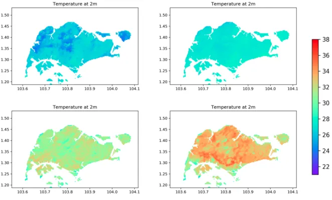
climatic variables at any temporal resolution in NetCDF format with the defined grid resolution. The grid is regular on a horizontal plane and uses pressure levels in the vertical direction. Therefore, the output can be expressed as a three or four-dimensional spatio-temporal matrix, whereby each entry in the matrix represents a grid cell of the WRF grid. For example, Figure 2.1.6 shows near-surface air temperature at 2 m for different times during a simulated day.
Cooling Singapore is using WRF to simulate Singapore’s urban climate and examine the UHI effect at a temporal resolution of one hour and a spatial resolution of 300 m. From the various climatic variables, Cooling Singapore uses predominantly the near-surface air temperature at 2 m for further analysis.
Figure 2.1.6: Example visualisation of a meteorological climate variable - near-surface air temperature at 2 m - at selected times (from top left to bottom right: 6 am, 9 am, 12 pm, 3 pm) extracted from the output of a WRF simulation of 2 April 2016. (Data source: Muhammad Omer Mughal, Cooling Singapore, 2020)
2.2 Microscale Urban Climate Model
Outdoor Thermal Comfort (OTC) is known as an important contributor to health and wellbeing. Studying OTC requires an understanding of the relationship between human physiology, climate and urban spaces. For quantitative assessment of different strategies on OTC improvement, Cooling Singapore conducts various microscale urban climate simulations using two different computational fluid dynamics
(CFD) modelling tools: ENVI-met and ANSYS Fluent. Both tools complement each other for assessing the impact of various mitigation strategies on urban climate. Cooling Singapore uses the Physiological Equivalent Temperature (PET) as the OTC index for the evaluation of different design scenarios. While ENVI-met facilitates the calculation of PET index, ANSYS Fluent can model heat transfer, such as anthropogenic heat dispersion.
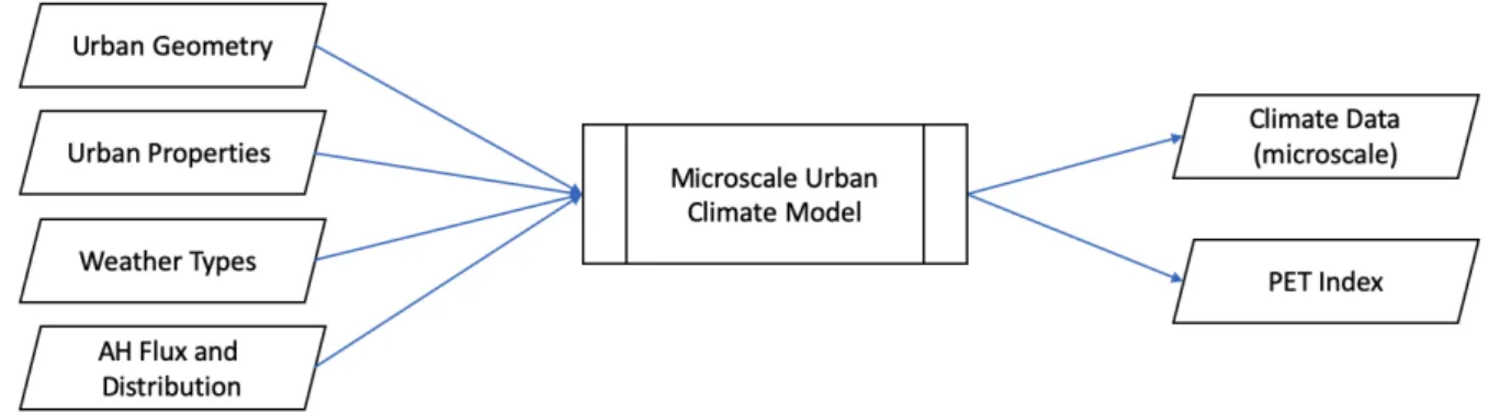
In the context of Cooling Singapore, the Microscale Urban Climate Model requires four main inputs:
Urban Geometry, Urban Properties, Weather Types and AH Flux and Distribution. It returns two output data objects: Climate Data (microscale) and the PET index. The inputs and outputs are visualised in Figure 2.2.1.
Figure 2.2.1: Principal inputs and outputs of the microscale urban climate model.
CFD simulations can generally run in two different modes: steady-state and transient. Simulations using steady-state mode compute the fully developed solution that does not change in time. Simulations using transient mode compute the temporal development of the climate over time. The latter has a higher demand for computational resources (primarily CPU time and disk storage). Depending on the goal of assessment and the availability of computational resources, simulations are conducted in different modes with different tools. In Cooling Singapore, simulations in transient mode are primarily conducted with ENVI-met for assessing the passive mitigation strategies such as urban form and vegetation cover.
Simulations in ANSYS Fluent are mainly run in the steady-state mode for evaluating the impact of AH.
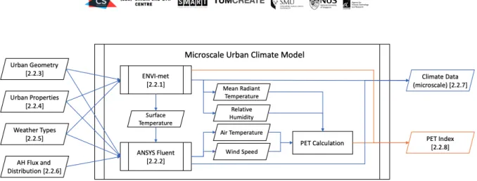
Due to the complexity of the ANSYS Fluent model, its computational time is much longer than ENVI- met for the same scenario and same simulation setting. In order to reduce the simulation time, researchers of Cooling Singapore aim to develop a coupling method between both models, which is visualised in Figure 2.2.2.
Figure 2.2.2: Illustration of the coupling of ENVI-met and ANSYS Fluent for calculating the PET index with the consideration of anthropogenic heat. ENVI-met provides surface temperature which is used by ANSYS Fluent as an initial condition. Using this method, the computational time of ANSYS Fluent can be reduced significantly.
(Source: adapted from Adelia et al., 2020)
The coupling method is still under development at the time of writing. See (Adelia et al., 2020) for details on the coupling approach. The remainder of this section describes the input and output data objects for the microscale urban climate model component. In addition, the two model sub-components, ENVI-met and ANSYS Fluent, are also explained. The function of PET calculation is still under development and thus not further explained here.
ENVI-met
ENVI-met8 is a three-dimensional CFD model designed to simulate the surface-vegetation-air interaction in an urban environment with a typical resolution of 0.5 - 10 m in space and 1 - 5 s in time (ENVImet, 2020). It calculates the temporal and spatial development of various climatic variables, such as air temperature, wind speed/direction, and relative humidity in outdoor spaces. This model has a built-in post-processing tool (BioMet9) that calculates the human thermal comfort indices directly from the climatic output of the simulated data. For example, this includes calculation of the Physiological Equivalent Temperature (PET) which is widely used for evaluating OTC. PET is calculated mainly using the following climatic variables: air temperature, mean radiant temperature, wind speed and relative humidity. Cooling Singapore uses ENVI-met primarily to evaluate the influence of mitigation strategies concerned with urban form and vegetation cover on the microclimate and OTC.
8 ENVI-met: https://www.envi-met.com
9 ENVI-met BioMet: http://www.envi-met.info/doku.php?id=apps:biomet
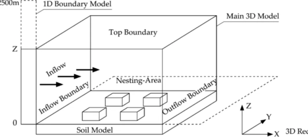
The ENVI-met model is composed of a one-dimensional boundary model, a 3D model of the area of interest and a soil model (see Figure 2.2.3). The one-dimensional boundary model is responsible for preparing the inflow and top boundary of the 3D model (Jin et al., 2017). The 3D model is divided into regular grid cells for the simulation. Despite being considered as one of the most comprehensive microclimate models, ENVI-met also has limitations. For example, it is unable to account for anthropogenic heat. Therefore, Cooling Singapore uses ANSYS Fluent to address this limitation.
Figure 2.2.3: Basic model layout of ENVI-met. (Source: Jin et al., 2017)
ANSYS Fluent
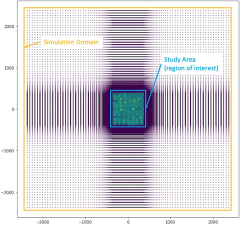
ANSYS Fluent10 is a more generic and widely used commercial CFD tool with the focus on modelling airflow, turbulence and heat transfer. Similar to ENVI-met, ANSYS fluent is widely used in urban climate studies and is capable of simulating climatic parameters such as relative humidity, air temperature and wind speed for outdoor spaces. However, unlike ENVI-met, ANSYS Fluent can incorporate anthropogenic heat sources requiring a much larger simulation domain than ENVI-met (Adelia et al., 2020). Figure 2.2.4 illustrates the simulation domain of ANSYS Fluent.
Due to the increasing model precision and domain size, ANSYS Fluent requires significantly higher computational resources and longer runtimes for the same design scenario. In Cooling Singapore, ANSYS Fluent is primarily used to assess the impact of AH release from various urban scenarios, such as different traffic scenarios and building cooling technologies. However, the calculation of PET index
10 ANSYS Fluent: https://www.ansys.com/products/fluids/ansys-fluent
with ANSYS Fluent is not straightforward since one of the main climatic variables mean radiant temperature, is not directly provided in the outputs of the simulation. Additional post-processing procedure for the PET calculation is developed within the project of Cooling Singapore.
Figure 2.2.4: Top view of the simulation domain in ANSYS Fluent. This simulation domain has a size of 5000 m x 5000 m while the study area is only around 500 m x 500 m.
Urban Geometry
Urban geometry directly affects local climatic conditions and thermal performance of urban spaces. This includes the building and canyon layout, the location of urban elements, the building height and geometry, and surface coverage. The arrangement of urban elements (e.g., buildings, canyons, trees) can affect the spatial coverage of the shadowed areas as well as the wind environment. These two aspects, in particular, are important for improving OTC and reducing the UHI in Singapore which generally experiences low wind speeds due to its geographical locations near the equator. Adequate wind flow can help remove accumulated heat (Ruefenacht and Acero, 2017). Cooling Singapore
developed various design scenarios with the objective to improve OTC at the pedestrian level (which is usually considered as 1 m above ground).
Information about urban geometry is provided by the 3D model of the study area. It is created using computer-aided design software and placed in the centre of the simulation domain (see Figure 2.2.4).
Prior to simulating, meshing is performed on the whole model domain (i.e., the main 3D model in Figure 2.2.3). Meshing is a process of dividing a large geometric space into a finite number of regions, namely grids or cells, in which the fluid dynamic equations are solved. The mesh quality is a key factor to determine the accuracy of the solutions generated (Adelia et al., 2020). Although ENVI-met and ANSYS Fluent can generate hexahedral structured mesh, each CFD tool applies its meshing algorithm based on user-defined parameters. Thus, the resulting meshes in different CFD tools have different representations.
ENVI-met creates a regular horizontal grid while the growth ratio only applies vertically. This creates a pixel-like grid with the same size for every grid cell on a horizontal plane (Adelia et al., 2020). Figures 2.2.5 shows the 3D model before and after the meshing process. It is important to note that not only the building objects will be discretised by the meshing, but the whole three-dimensional model domain including outdoor space will also be divided into grid cells (not shown in Figure 2.2.5). For Cooling Singapore, the horizontal grid size is defined as 3 m x 3 m and the cell height of the first 5 vertical levels is 2 m for each, while the resting cell height increases after every level. This finer cell height close to the ground surface can provide a more accurate and detailed solution on the pedestrian's level in OTC assessment. This type of grid allows OTC assessment on a horizontal plane at the selected height by creating a two-dimensional matrix where every entry corresponds to the grid cell on the domain and describes the simulated value of the cell in the output.
Figure 2.2.5: Urban geometry for a scenario of the elevated podium before (top) and after (bottom) the meshing.
The 3D model for the simulation can be created by using computer-aided design software or CFD tools. The top image visualises a 3D model of the scenario in Rhinoceros 3D. The bottom image shows the mesh of the same scenario in ENVI-met whereby the geometry of the scenario consists of mesh cells. (Source: Rhinoceros 3D (upper), ENVI-met Spaces (below))
The ANSYS Fluent grid, in contrast to ENVI-met, is irregular, as the mesh is generated based on user- defined parameters such as maximum size, growth ratio, initial cell size, the minimum number of cells for a surface, etc (Adelia et al., 2020). The evolved mesh consists of different sizes of cells on a
horizontal plane since the mesh is adjusted to the objects’ geometry, unlike the ENVI-met, where the objects’ geometry might be slightly adjusted to the mesh, as the ENVI-met mesh contains only cells with whole numbers. The ANSYS Fluent mesh is described by a list of point coordinates denoting the centres of the cells, described by its x, y, z coordinates. The data format of the mesh also defines the format of the simulation result (xi, yi, zi, Ti), where each mesh point (xi, yi, zi) is assigned with a simulated value Ti.
Urban Properties
Urban properties provide detailed information about the characteristics of urban elements (e.g., buildings, streets and open spaces) within the simulation domain, such as surface materials of the pavement and buildings, vegetation type, and soil type. These properties of the urban elements play an important role in the interaction with the boundary climate conditions and strongly influence the building energy demand for cooling, which is an important factor for tropical cities like Singapore. Appropriate surface materials can improve OTC and reduce UHI in an urban space, as it can lower the surface temperature of urban elements as well as surrounding air temperature and reduce the cooling energy consumption in buildings.
Weather Types
In microclimate CFD simulation, climatic boundary conditions initialise the model and specify the climatic behaviour and properties at the boundaries of the model domain. The assessment of OTC is generally conducted for a whole year to capture the effects of different seasons and variations in the climatic conditions. Rather than simulating an entire year, which is time-consuming and computationally expensive, Cooling Singapore uses representative climatic conditions, further referred to as weather types, instead. Weather types are obtained by applying a clustering method on the meteorological data of an entire year (Acero et al., 2020). After clustering, the characteristics of each weather type, including air temperature, wind speed and direction, relative humidity and cloud cover and frequency of occurrence, is derived from the data points of that cluster. In addition to using observation data from local weather stations, weather types can also be obtained by using EnergyPlus weather data11. Since ENVI-met simulations are transient and conducted for a period of 24 hours, the weather type file contains an hourly profile of air temperature and relative humidity which is fed into the 1D boundary model for creating the boundary conditions. In order to conduct the ANSYS Fluent simulation under the
11 EnergyPlus Weather Data: https://energyplus.net/weather
same climatic condition, which is steady, the inlet boundary condition for the ANSYS Fluent simulation is derived from the ENVI-met 1D boundary model at a chosen hour.
AH Flux and Distribution
In contrast to ENVI-met, ANSYS Fluent is capable of modelling the dispersion of anthropogenic heat released from different urban activities. It allows the users to import a heat flux profile that describes the amount of emitted heat per square metre (W/m2) and to specify the location of the emission. In Cooling Singapore, the estimation of anthropogenic heat is performed by other components, such as a building energy model (Section 2.4) or microscopic traffic model (Section 2.7). Those results need to be processed and converted into heat flux profile before being used by the ANSYS Fluent model, as the outputs from different models have different representations. For example, a building energy model, such as City Energy Analyst (Section 2.4), only calculates the total electricity consumed by each building in hourly resolution. Additional information such as Gross Floor Area and numbers of floors of the selected building is required for calculating the heat flux released by this building. Depending on the configuration of the design scenario, the heat is uniformly distributed over a surface where the heat is released. Figure 2.2.6 shows two examples of the spatial distribution of the released heat in ANSYS Fluent.
Figure 2.2.6: Illustrations of scenarios with a decentralised cooling system (left) and centralised cooling with cooling towers on rooftops (right). While a decentralised cooling system releases the heat over the facade of the buildings, a cooling tower releases the heat only on the rooftop. (Source: Aye Sukma Adelia and Lea Ruefenacht, Cooling Singapore, 2020)
Climate Data (microscale)
Climate models such as ENVI-met and ANSYS Fluent simulate the evolution of atmospheric variables in urban environments with the consideration of the influence of architecture, vegetation, surface characteristics, soils and climatic conditions. The outputs of these climate simulations include a range of climatic and environmental variables such as air temperature, relative humidity, ground surface temperature and wind speed, etc. In the OTC assessment, Cooling Singapore is specifically interested in the following climatic variables: air temperature, relative humidity, wind speed and direction and mean radiant temperature. These variables are the key parameters for the calculation of the PET value. The simulation output includes the state of these climatic variables with the defined mesh grid representation at each hour.
Each ENVI-met simulation generates a comprehensive state about the 3D model domain for each hour within the simulation period, therefore a large amount of simulation data is created and stored in binary format. For OTC assessment, the climatic variables of interest are extracted on the pedestrian level at the level of the grid cell closest to the ground and stored in a two-dimensional matrix. Figure 2.2.7 shows the extracted ENVI-met data for wind speed and direction at the pedestrian level at 12 pm.
Figure 2.2.7: Visualisation of wind speed and direction at 12 pm extracted from the simulation results of ENVI-met.
The wind speed is visualised with the colour field and its direction with black arrow. (Data source: Juan Angel Acero, Cooling Singapore, 2020)
Unlike ENVI-met, the ANSYS Fluent grid is irregular on a horizontal plane as shown in Figure 2.2.8, whereby the cell size varies in different locations. The grid cells are represented by point coordinates (x, y, z) of the cell centres, therefore, the simulation results are stored in the same format (x, y, z, T).
Due to the irregularity of the grid additional steps are needed to translate the data for comparison and evaluation.
Figure 2.2.8: Visualisation of simulated air temperature at 2 m from ANSYS Fluent. Shown are colour-coded points (centre of the mesh cell), indicating the air temperature. The distance between points increases the further points are from the origin mesh point, which makes the mesh irregular. (Data source: Aye Sukma Adelia, Cooling Singapore, 2020)
PET Index
Physiological Equivalent Temperature (PET) is a commonly used thermal index for measuring how thermal changes in an outdoor environment affects the health of humans. It is calculated based on a thermo-physiological heat balance model. PET calculation requires not only meteorological parameters such as air temperature, relative humidity, wind velocity and the mean radiant temperature but also individual parameters like clothing level and human activity (Höppe, 1999). Since PET index has a unit of temperature (°C), which is comprehended and easy to understand, it is widely used by urban planners for evaluating different design scenarios. Cooling Singapore is primarily using PET to measure the OTC performance of various design scenarios. As one of the important products of ENVI-met, PET is calculated by the ENVI-met Biomet model directly from its simulation output and is expressed as a four-dimensional spatio-temporal matrix (i.e., three spatial dimensions and time), similar data structure as the Climate Data (refer to Section 2.2.7).
2.3 Mesoscale Traffic Model
Rapid urbanisation and population growth lead to growth in traffic demand and the number of vehicles on the road. According to (Kayanan et al., 2019), the transport sector is a significant contributor to anthropogenic heat release based on its energy consumption. The mesoscale traffic model is built on a fluid-like model of traffic flow and is used to estimate the spatio-temporal distribution of AH emission caused by the traffic on the city-scale level. In the context of Cooling Singapore, the AH emission from the traffic is directly derived from the energy consumption of the moving vehicles on the roads. City Mobility Simulator (CityMoS) is a microscopic agent-based mobility simulator that allows for the evaluation of vehicle travel patterns and decision-making processes of the mobile entities. Cooling Singapore uses the flow-based mode of CityMoS to estimate the spatio-temporal energy consumption distribution caused by vehicles on the roads. CityMoS can be used to estimate the energy consumption by different transportation modes in Singapore, such as a mix of vehicles with various combustion engines (current state as baseline) or electrification of vehicles as well as autonomous vehicles (future scenarios).
The mesoscale traffic model requires three principal inputs (see Figure 2.3.1): Road Network, Traffic Demand and Vehicle Population Information. The model produces two major outputs: AH profile and Demand Variation. The generated AH Profile is used by the mesoscale urban climate model (Section 2.1) as input for the UHI assessment and the Demand Variation in electricity is used by the power plant dispatch model (Section 3.5) for additional AH assessment.
Figure 2.3.1: Principal inputs and outputs of the mesoscale traffic model.
The mesoscale traffic model component consists of two parts: the CityMoS model and the post- processing procedure required for transforming CityMoS simulation outputs into the required input data of the mesoscale climate model. The main components of the mesoscale traffic model are illustrated in Figure 2.3.2.
Figure 2.3.2: CityMoS and post-processing components as part of the mesoscale traffic model.
In the remainder of this section, the CityMoS model and its post-processing components will also be explained. In addition, each of the inputs and outputs illustrated in Figure 2.3.2 will also be explained in detail.
City Mobility Simulator (CityMoS)
CityMoS is a general-purpose agent-based road transport model with the microscopic level of detail which pertains to modelling the movement decisions of every single agent (vehicle) in the simulation as well as all kinds of interactions that arise from those movements. For the city-scale AH estimation, two submodules of CityMoS, Traffic Assignment Model and Vehicular Energy Consumption Model, have been mainly used for estimating the spatial distribution of released heat by the vehicles at each time step. CityMoS can execute the simulation in high temporal resolution defined by the user (Cooling Singapore uses an hourly resolution).
Traffic is simulated in a time-stepped fashion. At each time step, the traffic assignment model of CityMoS estimates the distribution of agents (i.e., road occupancy) on road segments as well as the road occupancy based on the traffic demand. Each agent is assigned vehicle characteristics (e.g., engine type, vehicle weight) defined by the Vehicle Population Information. Given the vehicle characteristics and the travel speed (subject to prevailing traffic conditions), the model can estimate the energy consumption of each agent. For scenarios with electric vehicles, CityMoS also simulates the additional demand for electricity which is needed for the assessment of AH emissions by the power generation sector.
Road Network
The road network represents the model domain and identifies the system of roads on which vehicles can travel. It does not include the rail network. The road network is structured as a directed graph
G(E,N) where the edges E represent the road segments and the nodes N connect two road segments.
In the simulation, the road network is divided into multiple road segments. Each road segment is a subregion of a road and is characterised with maximum allowed speed, length, road width and the number of lanes. Additionally, the road network contains shape information of the roads called lane information, such as the starting and ending point of the lane in the network, the lane shape, speed limit, and the neighbour road segment id. Figure 2.3.3 visualises the road transport network of Singapore used in CityMoS.
Figure 2.3.3 Road transport network of Singapore. (Source: Jordan Ivanchev, Cooling Singapore, 2020)
Traffic Demand
Traffic demand refers to the movement of people, vehicles and goods to satisfy a need such as work, education and economic activity. Travel demand used by Cooling Singapore is based on data from Singapore’s Household Interview Travel Survey, collected through the Public Transport Council. The dataset consists of trip information of about 50,000 commuters describing their movements for a single day, including walking, cycling, taking public transportations, being a passenger in a vehicle or driving a vehicle (Ivanchev and Fonseca, 2020). Only a subset of this data is thus relevant to determine road traffic demand. Trip information, including origin and destination postal codes, starting time and estimated trip duration, is used to construct an origin-destination matrix that is used by CityMoS to
generate traffic. At each time step, CityMoS can determine the locations of the agents and the occupancy of each road segment.
Vehicle Population Information
Vehicle Population Information describes the distribution of different vehicle types used by traffic simulation. Five major vehicle types are considered: private cars, lorries/vans, taxis, public buses, and motorcycles. Every vehicle type is characterised by physical attributes, such as mass, frontal area, drag coefficient, length, fuel type and vehicle engine type. In CityMoS, each vehicle is represented by an agent and is equipped with an energy consumption model defined by the vehicle type. Based on the vehicles’ velocity and acceleration, as well as the slope of the road segment, the energy consumption and heat emitted by the vehicle is calculated for each time step. The vehicle type for each agent or each trip is either defined by traffic demand or derived from the vehicle population information. This allows simulating scenarios with a certain mix of vehicle types (e.g., 50% private cars, 10% lorries, 15%
taxis, 15% public buses, and 10% motorcycles).
Energy Consumption per Road Segment
The energy consumption per road segment is an intermediate output of the mesoscale traffic model. It is the direct output of CityMoS that stores the simulated energy consumption of each road segment. In order to use this information for the urban climate simulation, this simulation output needs to be transformed into the correct data format.
Heat Conversion and Resampling
Heat Conversion and Resampling transforms Energy Consumption per Road Segment into an AH profile with the spatio-temporal resolution required by the mesoscale urban climate model. Cooling Singapore uses an hourly profile with a 300 m x 300 m spatial resolution. This function resamples the consumed energy on the road network into a grid. For each hour and grid cell, the total consumed energy for the road segments within the cell is aggregated and converted to heat flux (W/m2).
Anthropogenic Heat Profile (Road Transport Sector)
An Anthropogenic Heat Profile (AH Profile) for the road transport sector consists of multiple two- dimensional heat flux maps in hourly resolution. Each heat flux map represents the spatial AH emissions released by the vehicles for the corresponding hour of the day. As mentioned in Section 2.1.6, heat flux maps contain the height information of the heat sources. The heat produced by vehicles is assumed to be always released on the ground. In Cooling Singapore, mesoscale traffic simulations are conducted
for 24 hours and hence the resulting AH profile consists of 24 two-dimensional heat flux maps with a spatial resolution of 300 m defined by the mesoscale urban climate model. The AH profile is the product of the post-processing step described in section 2.3.6. Figure 2.3.4 visualises two examples of heat maps at different times of the day.
Figure 2.3.4 Anthropogenic heat flux maps for the whole city during the peak hour in the morning (a) and a non- peak hour at noon (b). Each pixel represents a WRF grid cell. (Source: Ivanchev and Fonseca, 2020)
Electricity Demand per Road Segment
Another intermediate output of the mesoscale traffic model is electricity demand per road segment. In a traffic scenario with electrified vehicles, the consumed energy is electricity. The electric vehicles require electricity supply provided by the power plants that release additional AH during electricity generation. This additional AH is not negligible. In the assessment of an electrification scenario, CityMoS simulates with electric vehicles on the roads and calculates the required electricity for each road segment. The required electricity by the vehicles determines the electricity demand of the traffic.
Aggregation
Another post-processing function involved in the mesoscale traffic model is the aggregation function. It transforms the electricity demand per road segment (Section 2.3.8) into an hourly electricity demand profile of the assessed scenario. For each hour, it aggregates the electricity demand on the road segments caused by the electrified vehicles over the island and creates a demand profile of electricity.
Figure 2.3.5 illustrates an example of the electricity demand profile for an electrification scenario.
Demand Variation (Road Transport Sector)
While the anthropogenic heat profile indicates the direct heat emitted on the roads, the indirect heat emission from the generation of the electricity consumed by electric vehicles also needs to be considered. A shift to electric vehicles also shifts the energy consumption from petrol/diesel fuel to electricity, consequently increasing heat emissions of the power plants due to additional electricity generation. In Singapore, electricity is mainly generated using natural gas which is more efficient than internal combustion engines. A shift to electric vehicles thus results overall in a net reduction of heat emissions. For assessing the impact of an electrification strategy, in which the vehicles in the simulation are replaced with electric vehicles, the temporal variation in electricity demand is calculated by comparing the electricity demand of the assessed scenario with the base scenario for each hour. This temporal variation in electricity demand will be considered by the power plant dispatch model (Section 2.5) for AH assessment. Electric vehicles have charging behaviour models that determine the moment charging will occur and the duration of the charging itself. This creates varying demand patterns for the hours of a day.
Figure 2.3.5: Electricity demand profile of a fully-electrified road transportation scenario with 20-kW charging stations for Singapore in 2016. (Source: Ivanchev and Fonseca, 2020)
2.4 Building Energy Model
As a high-density tropical city, the energy consumption by the building sector in Singapore constitutes approximately 12% of the country’s total energy consumed (Kayanan et al., 2019). The building sector covers residential, commercial and service buildings. A large portion of the building electricity consumption is caused by the use of air conditioning for cooling. While the use of air conditioning makes the heat of the tropics more bearable, the heat produced from the cooling systems (including waste heat due to cooling system inefficiencies) is released into the environment causing an increase in local air temperature. Cooling Singapore uses City Energy Analyst (CEA) to quantify the amount of heat released by buildings with different cooling systems, such as decentralised cooling systems, cooling tower and district cooling. The principal inputs and outputs of the mesoscale building energy model are illustrated in Figure 2.4.1.
Figure 2.4.1: Principal inputs and outputs of the mesoscale building energy model.
Due to the nature of the CEA model, simulations with CEA can only be conducted on a district scale.
To utilise the CEA model for mesoscale assessment on the city-scale level, additional post-processing procedures have been developed by Cooling Singapore. Figure 2.4.2 shows the major components of post-processing components within the mesoscale building energy model.
Figure 2.4.2: Illustration of the incorporation of district-scale CEA model and CEA-specific post-processing procedure for mesoscale assessment.
The application of the CEA model for mesoscale and microscale assessments in Cooling Singapore is very similar, thus both will be explained in this section. For the mesoscale assessment, the generated AH Profile and Demand Variation will be fed into mesoscale urban climate model and power plant dispatch models respectively. For the microscale assessment, the direct output of CEA District Heat Emission will be included into microscale urban climate models (i.e., ANSYS Fluent).
The remainder of this section will describe the CEA model and its main inputs/outputs in detail.
Furthermore, the description of the post-processing steps for transforming the simulation results from the district-level into city-scale level is also included.
City Energy Analyst (CEA)
CEA is a computational tool employed for the analysis and optimisation of energy systems from a single building to district scale. It applies energy balance and physical models of heat and mass flows to analyse the amount of energy consumed, carbon emissions and economic benefits among multiple design scenarios (Fonseca et al., 2016). The CEA tool is equipped with a user-friendly interface to guide its users from creating simulation scenarios and specifying the model inputs to analysing the simulation outputs. For the convenience of data inspection, all the inputs and outputs are saved in CSV format.
Due to the nature of CEA, simulations can only be conducted on district scale. The simulation with CEA requires three main inputs: District Geometry, District Properties and Meteorological Data as illustrated in Figure 2.4.2. CEA simulates the building energy usage that is emitted as heat into the environment and returns District Heat Emission data. In order to assess the impact of anthropogenic heat released by the building sector, an island-wide anthropogenic heat profile is required for mesoscale urban climate models. Instead of examining every building in Singapore which is computationally expensive, building energy simulations are only conducted on representative districts that are selected based on the LCZ map and building occupancy rates. Simulation data is then extrapolated (see Section 2.4.9).
District Geometry
District Geometry describes the spatial information of the district of interest, such as the shape and size of buildings, the geolocation of the district, its topography and morphology. This information is essential to construct a simple 3D model and can be extracted from OpenStreetMap12. CEA can also be applied to building models that have not yet been built by importing the corresponding shapefiles of the buildings. Compared to the urban geometry used in the microclimate simulation, the 3D model used in CEA is relatively simple. The energy consumption of buildings is also affected by their surrounding environment because of shading. Tall buildings in the surrounding cast more shade over the area of interest. The more the buildings in the area of interest are shaded, the less energy will be consumed.
Therefore, the complete model domain includes the buildings in the area of interest and their surrounding buildings, as illustrated in Figure 2.4.3.
12 OpenStreetMap: https://www.openstreetmap.org/
Figure 2.4.3. 3D building geometry of the simulation domain visualised in City Energy Analyst. The simulation domain contains the studied buildings (coloured in black) and the surrounding buildings (coloured in grey).
District Properties
District Properties contain architectural properties of all the buildings within the district, such as building materials, conditioned floor area and window-to-wall ratios, etc. It also includes general information, such as the construction year, renovation dates and functionality of the building, and the cooling technology used in the buildings. With the built-in OpenStreetMap API in CEA and its enriched database, this information is automatically extracted by CEA or specified by the users. Additional information would include the energy systems used in the buildings, indoor comfort properties, internal loads (e.g., water and electricity demand for various services) and the occupancy schedule (Mosteiro- Romero et al., 2019). The more information provided by the users, the more accurate the estimation of energy demand can be.
Meteorological Data (local)
Building energy demand is strongly influenced by ambient climatic conditions, such as solar radiation, relative humidity and wind. Local meteorological data for CEA is stored in EnergyPlus Weather13 format, a common data format for weather data used to run energy usage simulations. This data can be downloaded from the EnergyPlus website or generated using the Meteonorm14 software based on meteorological data that is either captured from weather stations or generated from microclimate modelling (Tsoka et al., 2019). These files contain meteorological data for one calendar year in hourly temporal resolution, same as the default simulation period of CEA.
Local Climate Zone Map
As explained in Section 2.1.2, an LCZ map provides land surface information and can be used to locate the building districts in Singapore. Most of Singapore’s LCZ types (8 of 10) correspond to buildings (i.e., LCZs 1-6, LCZ 8 and LCZ 9). Through the preliminary study of public available energy usage data of several districts, Cooling Singapore found that high variability in energy consumption pattern exists within the same LCZ type due to different occupancies. For example, LCZ 1 (compact high-rise) with dominating residential buildings has shown different energy usage than LCZ 1 with dominating commercial buildings. Therefore, subdivision of the same LCZ type is needed.
Cooling Singapore has developed a method to categorise an LCZ type into multiple district groups utilising additional land use information retrieved from the URA master plan15. The considered land-use information for buildings include commercial, residential (public and private). Each LCZ on the LCZ map is assigned additional land-use information and forms a new district group (LCZ type, land-use type) that creates a cluster of districts with lower variability in energy usage.
Conducting simulation for every building in Singapore is computationally expensive and practically not feasible. In order to create an island-wide AH profile using a district-scale model like CEA, Cooling Singapore conducts simulations on a selection of representative districts and later extrapolate the results to the entire city through the finer categorisation of LCZs. This approach can reduce the computational load and generate a city-wide anthropogenic heat profile. Therefore, a good selection of
13 EnergyPlus Weather Data: https://energyplus.net/weather
14 Meteonorm: https://meteonorm.com/
15 The masterplan of Singapore provided by URA: https://www.ura.gov.sg/maps/?service=mp
sample districts is crucial for an accurate estimation of the island-wide AH profile. From all categories of district groups, around 50 sample districts have been carefully chosen (see Figure 2.4.4).
Figure 2.4.4 Selection of representative sample districts, whereby different colours represent different LCZ types.
(Source: Luis Santos, Cooling Singapore, 2020)
District Heat Emission
District Heat Emission describes the amount of heat released by each building within the study district based on their electricity consumption profiles calculated by the CEA model. The CEA model calculates the electricity usage of each building in hourly resolution for a simulation period of one year and stores the results in CSV format. Depending on the occupancy patterns of the buildings and weather conditions throughout a year, electricity consumption of a building can vary between different months throughout the year and different times during the day. As a single-zone model, CEA calculates the total consumed electricity of a building without differentiating different usage between floors. Therefore, in the microscale assessment, additional processing of this simulation output is needed (refer to Section 2.2.6).