arXiv:1302.2936v1 [quant-ph] 12 Feb 2013
A quantum lens
Arseni Goussev1,2 and Klaus Richter3
1Department of Mathematics and Information Sciences,
Northumbria University, Newcastle Upon Tyne, NE1 8ST, United Kingdom
2Max Planck Institute for the Physics of Complex Systems, N¨othnitzer Straße 38, D-01187 Dresden, Germany
3Institute for Theoretical Physics, University of Regensburg, D-93040 Regensburg, Germany (Dated: February 14, 2013)
We consider the problem of quantum scattering of a localized wave packet by a weak Gaussian potential in two spatial dimensions. We show that, under certain conditions, this problem bears close analogy with that of focusing (or defocusing) of light rays by a thin optical lens: Quantum interference between straight paths yields the same lens equation as for refracted rays in classical optics.
PACS numbers: 03.65.Nk, 03.65.Sq, 42.25.Fx
I. INTRODUCTION
The intrinsic connection between the motion of classi- cal particles on one hand and the propagation of quantum matter waves on the other has occupied minds of scien- tists since the early days of quantum theory. De Broglie was one of the first to realize that “for both matter and radiations . . . it is necessary to introduce the corpuscle concept and the wave concept at the same time” [1].
Subsequently, invaluable contributions of Ehrenfest, Van Vleck, Feynman, Gutzwiller, Maslov, among many oth- ers, shaped our current understanding of quantum wave propagation in terms of interference of classical trajec- tories. However, a number of important questions con- cerning quantum-classical correspondence remain open.
These questions fall under the scope of the area of math- ematical physics known asquantum chaos [2–4].
The motion of a classical particle can be conveniently described by means of a phase-space trajectory. The Heisenberg’s uncertainty principle however does not al- low for the notion of the classical trajectory to be directly carried over to quantum theory: the particle’s position and momentum can not be specified simultaneously.
One natural extension of the classical concept of a point in the phase space is provided by a localized quan- tum wave packet that can be parametrized by its mean position and momentum, and dispersion quantifying the phase-space extent of the wave packet. According to the Ehrenfest theorem [5], the time evolution of the mean position and momentum is governed, for short enough times, by the classical equations of motion. In other words, the wave packet center follows the corresponding classical trajectory.
An issue of the wave packet spreading, i.e., how the dis- persion depends on time, is however much more complex.
Loosely speaking, there are two main mechanisms of the spreading: (i) a classical-like broadening of the wave packet due to forces exerted by an external potential, and (ii) an intrinsically quantum-mechanical spreading dictated by the uncertainty principle. Due to the inter-
ference nature of quantum dynamics, the overall spread- ing is not a simple “sum” of the two contributions, but rather a more intricate process.
A natural question arises: is there anintuitiveand, at the same time,quantitativetheoretical description of the phenomenon of quantum spreading? In this paper, we de- velop such a description, based on the short-wavelength approximation to quantum dynamics, for the simple sys- tem of a two-dimensional quantum wave packet scattered by a weak Gaussian potential. In particular, we show that the quantum scattering process bears a close math- ematical analogy with the phenomenon of focusing (or defocusing) of light rays by a thin lens, and can be de- scribed using the “language” of geometrical optics. In- terestingly, on the quantum side the use of the Eikonal approximation [6], i.e. including interference ofstraight paths, yields the same thin lens equation as derived in classical optics fromrefractedlight rays.
Our theoretical approach provides an intuitive picture of the wave packet spreading [7, 8], and its quantita- tive predictions are found in good agreement with results of an “exact” numerical solution of the time-dependent Schr¨odinger equation.
II. THEORY
We consider a quantum particle of massmthat evolves in the two-dimensional position space under the influence of the external potential
V(q) =V0e−q·Aq. (1) Here,V0 quantifies the strength of the potential, q is a column vector representing the particle’s position, and Ais a 2-by-2 orthogonal matrix with eigenvaluesa1and a2 corresponding, respectively, to orthonormal (column) eigenvectorse1 ande2. In other words,
A= (e1e2) diag(a1, a2) (e1e2)T, (2)
where|e1|=|e2|= 1 ande1·e2= 0. Hereinafter, the dot
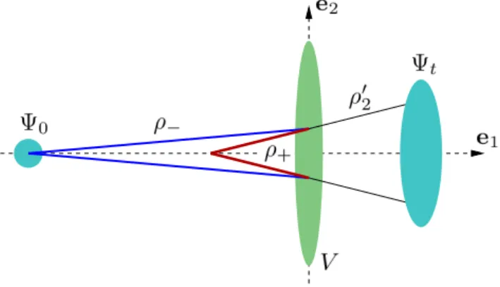
“·” stands for the scalar product, and the superscript “T” denotes the matrix transposition. Equation (1) describes a Gaussian potential “island” centered at q = 0, see Fig. 1. The spatial extent of the island is characterized by the lengthl1 = 1/√a1 in the direction of the vector e1 and byl2= 1/√a2in the direction ofe2.
FIG. 1: (Color online) Schematic illustration of the scattering system under consideration.
The dynamics of the quantum particle is fully de- scribed by its time-dependent wave function, Ψt(q). The latter is related to the initial wave function, Ψ0(q), by means of a propagatorKin accordance with
Ψt(q) = Z
dq′K(q,q′;t)Ψ0(q′). (3) Here, the q′-integration runs over the whole two- dimensional plane. In general, the propagatorKis deter- mined by solving the time-dependent Schr¨odinger equa- tion,
i~∂
∂t + ~2
2m∇2q−V(q)
K(q,q′;t) = 0, (4) subject to appropriate boundary and initial conditions, e.g., see Ref. [9]. Generally, this task is analytically formidable, and one is left to resort to numerical com- putations. In certain cases however analytical progress is made possible by constructing “sensible” approximations to the propagator. In this paper, we focus on one such approximation commonly referred to assemiclassics.
The semiclassical (or short-wavelength) approximation of the propagator K(q,q′;t) is formulated in terms of classical trajectories γ that start at the point q′ at time 0 and end at q at time t. More precisely, γ = {r(τ), τ∈[0, t]}, such that mdτd2r2 +∇V(r) = 0 with r(0) = q′ and r(t) = q. The approximate propagator, commonly referred to as the Van Vleck-Gutzwiller prop- agator, can be written as [2]
K(q,q′, t) = pDγ
2πi~ exp i
~Sγ−iπ 2νγ
, (5)
where
Sγ ≡S[r](t) = Zt
0
dτ (m
2 dr
dτ(τ) 2
−V r(τ) )
(6) is Hamilton’s principle function along the trajectoryγ,
Dγ=|det(−∇q′∇qSγ)| (7) is the stability factor ofγ, andνγ is the so-called Maslov index, counting the number of conjugate points alongγ;
as far as our problem is concerned, the Maslov index is identically zero,νγ = 0.
The approximation (5) is known to be reliable when applied to wave functions Ψ0(q) representing a quantum particle of sufficiently high kinetic energy E0. We ad- ditionally assume that the Gaussian potential, given by Eq. (1), is weak compared to the particle’s kinetic en- ergy, |V0| ≪ E0. The validity of this condition is at the heart of our “shallow potential island” approximation corresponding to the Eikonal approximation in scatter- ing theory [6]. In this case (see Appendix A),Sγ can be well approximated bySγ0, whereγ0is the straight, free- particle trajectory leading from q′ to q in time t, i.e., γ0={qτ /t+q′(1−τ /t), τ ∈[0, t]}. Thus, we write
Sγ ≃Sγ0 = m
2t|q−q′|2− Z t
0
dτ V q′+τ
t(q−q′) . (8) The integral in the right-hand side of Eq. (8) can be straightforwardly evaluated to equal
√πV0t 2A exp
−(q·Aq)(q′·Aq′)−(q·Aq′)2 A2
×
erf
q·A(q−q′) A
−erf
q′·A(q−q′) A
(9) with
A ≡p
(q−q′)·A(q−q′). (10) Expression (9), and therefore Eq. (8), can be further sim- plified by taking into account the identity
(q·Aq)(q′·Aq′)−(q·Aq′)2=|q×q′|2detA, (11) where “×” denotes the vector product. This yields
Sγ ≃ m
2t|q−q′|2−
√πV0t 2A exp
−|q×q′|2detA A2
×
erf
q·A(q−q′) A
−erf
q′·A(q−q′) A
. (12) A substitution of Eq. (12) into Eq. (5) leads to an ex- plicit, closed-form expression for the semiclassical prop- agator,K(q,q′, t), and, therefore, provides the complete solution of the time-dependent scattering problem in the short-wavelength regime.
The expression for the propagator,K(q,q′, t), becomes especially simple and allows for an intuitive interpreta- tion in the following special case. Let us consider a setup, in which the “receiver”qand the “source”q′ lie on the opposite sides of and at almost the same distance, large compared tol1, from the center of the Gaussian scatter- ing potential, and in which the vector (q−q′) is nearly aligned with one of the principal directions (taken, for concreteness, to bee1) of the potential island. In other words, we are interested in the asymptotic form of the functionK(q,q′, t) in the case that
q=Le1+ξ, q′=−Le1+ξ′ (13) and
|ξ|,|ξ′|, l1≪L . (14) Substituting Eq. (13) into Eqs. (10) and (12), taking into account that erf(±z)→ ±1 asz→+∞, and keeping only terms to the leading order in|ξ|/Land|ξ′|/Lin the argument of the exponential function, we obtain
Sγ ≃m
2t|2Le1+ξ−ξ′|2
−
√π 2
l1
LV0texp
−|e1×(ξ+ξ′)|2 (2l2)2
. (15) Then, using the basis representationsξ=ξ1e1+ξ2e2and ξ′=ξ′1e1+ξ2′e2 in Eq. (15), and further assuming that
ξ2, ξ2′ ≪l2, (16) we write, approximately,
Sγ ≃ −
√π 2
l1
LV0t+Sγ(1)+Sγ(2), (17) where
Sγ(1)= m
2t(2L+ξ1−ξ1′)2 (18) and
Sγ(2)= m
2t(ξ2−ξ2′)2+
√π 8
l1
L(l2)2V0t(ξ2+ξ2′)2. (19) In view of Eqs. (17–19), the stability factor (7) along the trajectoryγ can be written asDγ ≃D(1)γ Dγ(2), with Dγ(1)=|−∂ξ1∂ξ′1Sγ(1)|=m/tandDγ(2)=|−∂ξ2∂ξ′2Sγ(2)|= m/t−√πl1V0t/(4L(l2)2), provided that
t2≪ m(l2)2
|V0| L l1
. (20)
In fact, Eq. (20) states a necessary condition for Eq. (19) to constitute a “healthy” perturbative expansion ofSγ(2)
in powers ofV0.
The full semiclassical propagator, Eq. (5), can now be written as
K(q,q′,t)≃exp
−i
√π 2
l1
L V0t
~
×K0(L+ξ1,−L+ξ′1;t)KV(ξ2, ξ2′;t), (21) where
K0(z, z′, τ)≡ r m
2πi~τ exp i m
2~τ(z−z′)2
(22) is the free-particle propagator describing the motion of the particle in thee1-direction, while
KV(z, z′, τ)≡K0(z, z′, τ) s
1−
√π 4
l1
L V0τ2 m(l2)2
×exp
i
√π 8
l1
L V0τ
~
(z+z′)2 (l2)2
(23) accounts for the wave function spreading in the orthogo- nal,e2-direction. Clearly,KV →K0 as V0→0, recover- ing the free-particle limit.
We now observe that KV(z, z′, τ) =
Z +∞
−∞
dζ K0(z, ζ, τ /2)
×exp
"
i
√π 2
l1
L V0τ
~
1−
√π 4
l1
L V0τ2 m(l2)2
−1 ζ2 (l2)2
#
×K0(ζ, z′, τ /2). (24)
Equation (24) is an identity, and can be verified straight- forwardly by evaluating the Gaussian integral in the right-hand side. Then, after Eq. (20) is taken into ac- count, Eq. (24) reduces to
KV(z, z′, τ)≃ Z +∞
−∞
dζ K0(z, ζ, τ /2)
×exp
i
√π 2
l1
L V0τ
~ ζ2 (l2)2
K0(ζ, z′, τ /2). (25) The physical picture offered by Eq. (25) is as follows.
The propagator KV, evolving a quantum state during timeτ, can be view as a result of three consecutive opera- tions: (i) a free-particle propagation during timeτ /2, (ii) an instantaneous phase change, or “kick”, of the quantum state, and (iii) another free-particle propagation during τ /2. This interpretation, and the physical meaning of the kick operator, becomes apparent when the evolving quantum state is given by a Gaussian wave packet. To this end, we consider as initial state the two-dimensional wave packet
Ψ0(ξ1′, ξ2′)≡ψ0(1)(ξ1′;ρ1)ψ(2)0 (ξ′2;ρ2) (26) with
ψ0(1)(z;ρ)≡ 1
πσ2 14
exp
imv
~ z2
2ρ+z
, (27) ψ0(2)(z;ρ)≡
1 πσ2
14
exp
imv
~ z2 2ρ
. (28)
Here,ρ1 and ρ2 (usually termed radii of curvature [10]) are two, generally complex-valued, parameters. The real- valued functionσ=σ(ρ), defined in accordance with
1 σ2 ≡ mv
~ ℑ 1
ρ
=−mv
~ ℑρ
|ρ|2, (29) quantifies the position-space dispersion of the wave packet. Furthermore, v specifies the average velocity (andmv the average momentum) of the particle.
Now, acting with the propagator (21) on the initial state (26), which is assumed to be spatially localized around the position vector q′ = −Le1 (or around the origin in the ξ′-coordinate frame), we obtain the quan- tum state after timetlocally, in the vicinity of the point q=Le1(or around the origin in theξ-coordinate frame):
Ψt(ξ1, ξ2)≃e−i
√π 2
l1 L
V0t
~ ψ(1)t (ξ1;ρ1)ψt(2)(ξ2;ρ2), (30) where
ψ(1)t (z;ρ)≡ Z +∞
−∞
dζ K0(L+z,−L+ζ, t)ψ0(1)(ζ;ρ), (31) ψ(2)t (z;ρ)≡
Z +∞
−∞
dζ KV(z, ζ, t)ψ(2)0 (ζ;ρ). (32) As we are concerned with the semiclassical limit, it is rea- sonable to expect that, in the course of its time evolution, the quantum wave packet remains concentrated around the corresponding classical trajectory. This means that the center of the wave packet, starting from the point
−Le1 at time 0, reaches the point Le1 in time t, such that
vt= 2L . (33)
It is at this instant that Ψt(ξ1, ξ2) is localized around the origin in theξ-coordinate frame, and that the propagator approximation, given by Eq. (21), proves the most useful.
Fixing the timetin accordance with Eq. (33) and eval- uating the Gaussian integral in Eq. (31), we obtain
ψt(1)(z;ρ1) =eiφ1ψ0(1)(z;ρ1+vt), (34) whereφ1=E0t/~−(1/2) arg(1 +vt/ρ1), and
E0≡ mv2
2 , (35)
denoting the kinetic energy of the corresponding clas- sical particle. The physical interpretation of Eq. (34) is that the e1-component of the wave packet retains its Gaussian shape, as its center travels in space on top of the corresponding classical trajectory (and in agreement with the Ehrenfest theorem). The spreading of the e1- component of the wave packet is entirely described by the linear transformation of the corresponding radius of curvature,ρ1→ρ1+vt, and, in the weak potential limit, this spreading is not affected by the external potential.
We now focus on the time evolution of the e2- component of the wave packet. As before, we keep the time t fixed in accordance with Eq. (33). Substituting Eq. (25) into Eq. (32), and successively evaluating two Gaussian integrals, we obtain
ψt(2)(z;ρ2) =eiφ2ψ0(2)(z;ρ′2), (36) whereρ′2=ρ++vt/2,
1 ρ+
= 1 ρ−
+ 1
f , (37)
ρ− =ρ2+vt/2,
f ≡ 1
√π E0
V0
(l2)2 l1
, (38)
andφ2=−(1/2)
arg(ρ′2/ρ+) + arg(ρ−/ρ2) .
The physical picture of the wave packet spreading, offered by the central Eqs. (36–38), bears close anal- ogy with the focusing (or defocusing) of light rays by a thin optical lens. Indeed, the well-known thin lens equation, [object distance]−1+ [image distance]−1= [focal length]−1, can be readily recovered from Eq. (37) by interpreting−ρ− andρ+ as the “distances” from, re- spectively, the object and its image to a lens of the focal lengthf; the role of the lens is played here by the Gaus- sian potential island, see Fig. 1.
It is important to point out that the above analogy between the wave packet scattering in quantum mechan- ics and the ray focusing in optics is not a trivial one: in the quantum-mechanical case, the “distances”−ρ− and ρ+ are intrinsically complex-valued and can only be re- lated to the true distances, encountered in optics, in a nonlinear way.
Finally, we note that our simple wave-packet- propagation construction can be generalized to arbitrary times t. This generalization can be summarized as fol- lows. Suppose that the initial wave packet is centered around a point with coordinates (Q,0), where Q < 0, and that the initial wave function is given by the prod- uctψ0(1)(q1−Q;ρ1)ψ0(2)(q2;ρ2). Then, at a later time t, the wave function is given, up to an overall phase factor, byψ0(1)(q1−Q−vt;ρ1+vt)ψ(2)0 (q2;ρ′2), where
ρ′2=
ρ2+vt , t <|Q|/v
ρ++v(t− |Q|/v), t≥ |Q|/v (39) andρ+ is determined from Eq. (37) withρ−=ρ2+|Q|.
III. NUMERICAL CONFIRMATION We now confirm the validity of the “quantum lens”
formulae, given by Eqs. (37), (38), and (39), by com- paring their predictions to results of numerical simula- tions. The latter were performed by solving the time- dependent Schr¨odinger equation, governing the evolu- tion of the wave packet, numerically, using the method
of expanding the propagator in a series of Chebyshev polynomials of the Hamiltonian. The reader is referred to Refs. [11–13] for a comprehensive description of the method and its implementations.
The concrete system that we consider is schemati- cally illustrated in Fig. 1 and described by the following set of parameters. Hereinafter, we adopt atomic units,
~ = m = 1. The external Gaussian potential, Eq. (1), is characterized by l1 = 0.1 and l2 = 1, and the po- tential strength V0 plays the role of a variable param- eter, with values ranging between 10 and 40. The ini- tial state of the particle is given by the wave function ψ(1)0 (q1−Q;ρ1)ψ0(2)(q2;ρ2) withQ=−0.8,v = 60, and ρ1=ρ2=−i(mv/~)(σ0)2, whereσ0= 0.1 quantifies the initial position-space dispersion of the wave packet, cf.
Eq. (29). Note that the kinetic energy of the classical particle E0 = mv2/2 = 1800 is large compared to the strength of the external potential.
0 0.005 0.01 0.015 0.02 0.025 0.03 0.035 0
1 2 3 4 5 6 7 8x 10⁻⁴
t
∆σ2
V0= 40 (exact) V0= 40 (lens) V0= 30 (exact) V0= 30 (lens) V0= 20 (exact) V0= 20 (lens) V0= 10 (exact) V0= 10 (lens)
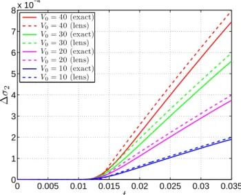
FIG. 2: (Color online) Spreading of the wave packet in the direction orthogonal to the direction of propagation. See text for details.
Our aim is to study the wave packet spreading in the direction orthogonal to the propagation direction. This spreading is given by the time-dependence of the disper- sion along thee2-axis,
σ2= s
2 Z
dq(q2)2|Ψt(q)|2. (40)
(Note that, due to the symmetry of Ψt(q) under the re- flection q2 → −q2, the expectation value of q2 is zero, i.e., R
dqq2|Ψt(q)|2 = 0.) For our choice of the initial state, σ2 =σ0 at t = 0, and σ2 increases as a function of time. In the limitV0= 0, this increase is determined by the free-particle spreading, σfree2 =σ(ρ2+vt), with the functionσ(ρ) defined by Eq. (29). A straightforward
calculation yields
σ2free= s
(σ0)2+ ~t
mσ0
2
. (41)
In the caseV0 6= 0, the external potential causes addi- tional spreading that can be quantified by
∆σ2≡σ2−σfree2 . (42) Figure 2 shows the dependence of ∆σ2 on time t for four different potential strengths, V0 = 10 (blue), 20 (magenta), 30 (green), and 40 (red). The solid curves represent the results of the “exact” numerical solution of the time-dependent Schr¨odinger equation, while the dashed curves show the analytical “lens” approximation, namely σ(ρ′2)−σfree2 with ρ′2, calculated in accordance with Eqs. (39), (37), and (38). As expected, ∆σ2 ≃ 0 for t . |Q|/v ≃ 0.013, corresponding to the time that it takes for the classical particle to reach the potential island. Figure 2 shows the theoretical predictions to be in a reasonable agreement with the numerical results. It also confirms that the agreement improves as the poten- tial strength is decreased.
IV. DISCUSSION AND CONCLUSIONS In this paper, we have constructed an approximate an- alytical solution to the problem of a scattering of a lo- calized quantum wave packet by a weak Gaussian poten- tial. Our solution is valid in the semiclassical regime, in which the particle’s de Broglie wavelength can be con- sidered short compared to all other length scales of the system. We have shown that the quantum scattering process is closely analogous to the phenomenon of focus- ing (or defocusing) of light rays by a thin optical lens.
In particular, the mathematical formula quantifying the wave packet spreading, Eq. (37), is largely equivalent to the thin lens formula of geometrical optics. The main difference between the thin lens formula in optics and Eq. (37) is that the former operates with true real-valued distances from the lens to the object and to the image, while the “distances” ρ− and ρ+ entering Eq. (37) are intrinsically complex-valued. It is only in the classical limit,mv/~→ ∞, that ρ− and ρ+ become real-valued, and that the optical thin lens formula is recovered.
It is instructive to further compare the ray optics pic- ture with our quantum mechanical result. The thin lens formula in optics, which is the classical limit of Eq. (37), effectively describes the deflection, or bending, of light rays (classical trajectories), induced by the lens (external potential). However, only straight, unbent trajectories have been used in our semiclassical derivation of Eq. (37).
This seeming paradox is resolved by the following ar- gument, originally presented in Ref. [14] and for read- ers’ convenience reproduced in Appendix A. The main building block of the semiclassical propagator, Eq. (5),
is the Hamilton’s principal function along the classical trajectory connecting the initial and final points of the propagation. However, in a sufficiently weak external potential, the value of the Hamilton’s principal function along the true (generally bent) classical trajectory is very close to that along the corresponding straight (unbent) trajectory, making the precise geometrical shape of the trajectory unsubstantial.
The approach taken in this paper is conceptually sim- ilar to the one used in Ref. [10] to analyze the spreading of quantum wave packets in the Lorentz gas. The latter consists of a particle moving in an array of fixed elastic scatterers, taken to be hard disks (spheres) in two (three) spatial dimensions. However, it is important to point out that in the Lorentz gas, unlike in the system addressed in the present paper, one must take into account deflections of classical trajectories in order to obtain the quantum- mechanical equivalent of the circular (spherical) mirror formula.
Acknowledgments
The authors thank Tobias Kramer for useful discus- sions. A.G. acknowledges the hospitality of the Uni- versity of Regensburg during a two-month visit where much of this work was done. K.R. thanks the Deutsche Forschungsgemeinschaftfor financial support within Re- search Unit FOR 760.
Appendix A: Expansion of Hamilton’s principal function
The following discussion is based on the argument that was, e.g., presented in Ref. [14].
Let us consider the Lagrangian Lǫ[r](τ) = m
2 dr
dτ(τ) 2
−ǫV r(τ)
(A1) along a trajectoryr(τ). Hereǫ ≪1 serves as a dimen- sionless strength of the potential. The corresponding Hamilton’s principal function is given by
Sǫ[r](t) =
t
Z
0
dτLǫ[r](τ). (A2)
We now denote by rǫ(τ) a trajectory that satisfies the boundary conditionsrǫ(0) =q′andrǫ(t) =q, and makes the actionSǫ[r](t) stationary, i.e.,
δSǫ
δr [rǫ](τ) =0. (A3) Then, for a trajectory r0(τ), that satisfies the same boundary conditions,r0(0) =q′ andr0(t) =q, and that is the stationary trajectory ofS0[r](t), we have
Sǫ[r0](t) =Sǫ[rǫ](t) + Z t
0
dτδSǫ
δr [rǫ]·(r0−rǫ) +1
2 Zt
0
dτ(r0−rǫ)·δ2Sǫ
δr2 [rǫ] (r0−rǫ) +. . . . (A4) Substituting Eq. (A3) into (A4) and taking into account rǫ=r0+O(ǫ) we obtain
Sǫ[rǫ](t) =Sǫ[r0](t) +O(ǫ2). (A5)
[1] L. de Broglie,The wave nature of the electron, Nobel Lec- ture (1929), avaliable onlinehttp://nobelprize.org.
[2] M. C. Gutzwiller,Chaos in Classical and Quantum Me- chanics (Springer-Verlag, New York, 1990).
[3] H.-J. St¨ockmann, Quantum Chaos: An Introduction (Cambridge University Press, Cambridge, 1999).
[4] F. Haake, Quantum Signatures of Chaos (Springer, Berlin, 2010).
[5] See, e.g., D. J. Tannor, Introduction to Quantum Mechanics: A Time-Dependent Perspective (Palgrave Macmillan, 2007).
[6] J. J. Sakurai, Modern Quantum Mechanics (Addison- Wesley, Reading, MA, 1994), pp. 392–394.
[7] For related work see: G. Vandegrift, Am. J. Phys. 72, 404 (2004).
[8] For an account of various semiclassical Gaussian wave
packet approaches see, e.g., E. J. Heller, Acc. Chem. Res.
39, 127 (2006).
[9] G. Barton,Elements of Green’s Functions and Propaga- tion(Clarendon Press, Oxford, 1989).
[10] A. Goussev and J. R. Dorfman, Phys. Rev. E71, 026225 (2005).
[11] H. Tal-Ezer and R. Kosloff, J. Chem. Phys. 81, 3967 (1984).
[12] H. De Raedt, J. S. Kole, K. F. L. Michielsen, and M. T.
Figge, Comp. Phys. Comm.156, 43 (2003).
[13] W. van Dijk, J. Brown, and K. Spyksma, Phys. Rev. E 84, 056703 (2011).
[14] O. Bohigas, M.-J. Giannoni, A. M. O. de Almeida, and C. Schmit, Nonlinearity8, 203 (1995).