a Signature of Quantum Many-Body Interference in Interacting Bosonic Systems

(1)

a Signature of Quantum Many-Body Interference in Interacting Bosonic Systems

Thomas Engl,¹ Julien Dujardin,² Arturo Arg¨uelles,² Peter Schlagheck,² Klaus Richter,¹and Juan Diego Urbina¹

1Institut f¨ur Theoretische Physik, Universit¨at Regensburg, D-93040 Regensburg, Germany

2Département de Physique, Université de Liège, 4000 Liège, Belgium

We predict a generic manifestation of quantum interference in many-body bosonic systems resulting in a coherent enhancement of the average return probability in Fock space. This enhancement is both robust with respect to variations of external parameters and genuinely quantum insofar as it cannot be described within mean-field approaches. As a direct manifestation of the superposition principle in Fock space, it arises when many-body equilibration due to interactions sets in. Using a semiclassical approach based on interfering paths in Fock space, we calculate the magnitude of the backscattering peak and its dependence on gauge fields that break time-reversal invariance. We confirm our predictions by comparing them to exact quantum evolution probabilities in Bose-Hubbard models, and discuss the relevance of our findings in the context of many-body thermalization.

PACS numbers: 03.65.Sq, 05.45.Mt, 67.85.-d, 72.15.Rn

The existence of a superposition principle for quantum states is a cornerstone in our picture of the physical world, with observable implications in the form of coherent phenomena that have been experimentally demon- strated with impressive precision during the last century [1–3]. Within the context of linear wave equations, quantum superposition effects represent particular cases of the general phenomenon of wave coherence. For quantum systems described by the single-particle Schr¨odinger equation, this analogy between quantum and classical waves was exploited to demonstrate coherent quantum effects, such as Anderson localization in disordered metals [4] or coherent backscattering (CBS) [5], by using classical (in particular electromagnetic) wave analogues [6–8].

In the quantum description of many-body systems, such an analogy between quantum dynamics and classical wave phenomena does not hold. Within a first-quantized approach, the quantum mechanical description of a system of N interacting particles inD dimensions requires us to extend the space in which the Schr¨odinger field ψ(~r1, . . . , ~rN, t) is defined to N D dimensions. We can still identify the quantum superposition principle with the linearity of the many-body Schr¨odinger equation, but the latter does no longer describe a classical wave in real D-dimensional space: Many-body quantum interference is a high-dimensional phenomenon.

This observation remains true even if we adopt a real- space description in terms of the quantum field ˆψ(~r, t).

Indeed, ˆψ(~r, t) is an operator instead of a complex amplitude and does not represent a quantum state. Nev- ertheless, quantum fields are a suitable starting point to implement approximations to the full many-body problem in terms of classical wave equations for single particles, which effectively amounts to the substitution ψ(~ˆ r, t) → ψ(~r, t) at the level of the Heisenberg equations of motion for ˆψ(~r, t). This approach leads to the mean-field Gross-Pitaevskii equation (GPE) [9] and also to the Truncated Wigner method [10–13] with its quan-

n⁽ⁱ⁾ n^(f)

n^(f)=n⁽ⁱ⁾

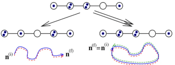
FIG. 1. (Color online) Illustration of Coherent Backscatter- ing in Fock space. A many-body system, represented here by a Bose-Hubbard chain withL= 5 sites andN = 6 particles, is prepared in a well-defined initial Fock state n⁽ⁱ⁾ = (n⁽ⁱ⁾₁ , . . . , n⁽ⁱ⁾_L) (upper part). After a given evolution time t, the final populations are found to be n^(f) (lower parts). A solutionγ of the Gross-Pitaevskii equation joiningn⁽ⁱ⁾ with n^(f)contributes with an amplitudeKγ'Aγe^iR^γ to this pro- cess, whereRγ is a classical action. Under averaging, only pairs of identical Fock space trajectories yield a systematically nonvanishing contribution to the probabilityP =|P

γKγ|² whenn^(f)6=n⁽ⁱ⁾(left column). Forn^(f)=n⁽ⁱ⁾(right column), however, constructive interference additionally arises if trajectories are paired with their time-reversed counterparts (dot- dashed green line). This gives rise to a coherent enhancement of the probability to detect the system in the initial Fock state after the evolution, as compared to other states with comparable distributions of the population.

tum (Wigner-Moyal) corrections [14]. Since the GPE is a classical field equation, its nonlinearity does not pose a conflict with the linearity of quantum evolution. For the same reasons, however, theψ(~r, t) field cannot represent a quantum state and its physical meaning requires further interpretation as a condensate fraction or order parame- ter. In particular, interference effects resulting from the (weakly nonlinear) GPE arenota consequence of many- body interference; they areclassical waveeffects proper of a classical field equation and are generically suppressed already for small interactions [15–18].

In this paper we report a semiclassical description

arXiv:1306.3169v1 [cond-mat.quant-gas] 13 Jun 2013

(2)

of the quantum mechanism responsible for many-body interference phenomena in interacting bosonic systems, which is schematically illustrated in Fig. 1. Our approach is based on coherent sums overmultiple solutionsof the GPE in occupation number space. It predicts quantum coherence effects which are in quantitative agreement with numerical simulations of Bose-Hubbard models describing cold atoms in optical lattices.

Since many-body interference is most visible in genuine many-body observables (i.e., which cannot be writ- ten as sums of expectation values of single-particle operators), we will study, as a representative example, the microscopic evolution probability from one many-body state to another one. Following standard techniques [19], we introduce a discrete and orthogonal but otherwise arbitrary set of Lsingle-particle states (”orbitals”) χ1, . . . , χL. The associated set of commuting bosonic occupation number operators ˆnαhas common (Fock) eigenstates|ni=|n1, . . . , nLiand integer eigenvalues nα de- noting the number of particles in each single-particle or- bitalχ_α. The transition probability between Fock states at timet reads then

P(n^(f),n⁽ⁱ⁾, t) =|hn^(f)|Uˆ(t)|n⁽ⁱ⁾i|², (1) with ˆU(t) ≡ exp(−iHt/ˆ ~) and the general many-body Hamiltonian exhibiting two-body interaction

Hˆ =X

αβ

h_αβˆa^†_αaˆ_β+1 2

X

αβησ

V_αβησˆa^†_αaˆ_βaˆ^†_ηˆa_σ, (2) which is expressed in terms of the ladder operators ˆ

aα(â^†_α) that annihilate (create) a particle in the orbital χα(with ˆnα= â^†_αâα). We shall later on refer to the more specific case of a Bose-Hubbard (BH) model describing, e.g., cold atoms in optical lattices, which corresponds to the choice

HˆBH=X

α

αnˆα−JX

α

(eîφâ^†_αâα+1+ e^−iφâ^†_α+1âα) +U

2 X

α

ˆ

nα(ˆnα−1). (3)

Our calculation (see [20] for details) is based on an asymptotic expansion of the many-body propagator,

K^sc(n^(f),n⁽ⁱ⁾, t)' hn^(f)|Uˆ(t)|n⁽ⁱ⁾i, (4) which is formally valid for n^(i,f)α 1. To this end, we have to consider all solutions (indexed byγ)

ψ^(γ)(s)≡ψ^(γ)(s;n^(f),n⁽ⁱ⁾, t)≡[ψ^(γ)₁ (s), . . . , ψ^(γ)_L (s)]

(5) of the mean-field Gross-Pitaevskii equation (GPE)

i~

∂

∂sψ_α=X

β

h_αβψ_β+X

βησ

V_αβησψ_βψ^∗_ηψ_σ (6)

that instead of initial conditions satisfy the bilateral boundary (or shooting) conditions|ψα(0)|²=n⁽ⁱ⁾α + 1/2 and |ψα(t)|² = n^(f)α + 1/2 and have argψα=1(0) = 0 [20]. In terms of those solutionsψ^(γ)(s), the semiclassical propagator is then expressed as

K^sc(n^(f),n⁽ⁱ⁾, t) =X

γ

A^(γ)exp[iR^(γ)+iπΦ^(γ)/4] (7) where, for each solution, the semiclassical amplitude

A^(γ)(n^(f),n⁽ⁱ⁾, t) = s

det⁰ 1 2π

∂²R^(γ)(n^(f),n⁽ⁱ⁾, t)

∂n^(f)∂n⁽ⁱ⁾

, (8) is given by the (dimensionless) classical action

R^(γ)(n^(f),n⁽ⁱ⁾, t) = (9)

Z t

0

X

α

θ_α^(γ)(s) ˙I_α^(γ)(s)−H[ψ^(γ)(s)]/~

! ds

withψα^(γ)(s)≡ q

Iα^(γ)(s) exp[iθα^(γ)(s)] and H(ψ) =X

αβ

hαβψ_α^∗ψβ+1 2

X

αβησ

Vαβησψ^∗_αψ_η^∗ψβψσ (10) the classical (mean-field) Hamiltonian. The Morse index Φ^(γ) counts the number of conjugate points along the trajectory γ. As indicated by det⁰, the derivatives in Eq. (8) are to be taken with respect to n^(i/f)₂ , . . . , n^(i/f)_L with n^(i/f)₁ being fixed by the total number of particles [20].

The heuristic use of H(ψ) as the classical limit in bosonic systems has a long history [21] and lies be- hind most studies of the quantum-classical correspon- dence in Bose-Hubbard models [12–14, 22]. However, a rigorous approach in which a semiclassical propagator is constructed by a stationary phase analysis of the exact path-integral representation of ˆU(t) in the spirit of the van Vleck-Gutzwiller approach for first-quantized systems [23] was missing in previous studies. Importantly, our propagator K^sc is valid also if the classical limit is non-integrable, thus going beyond the successful WKB method of Refs. [24, 25] forL= 2 and the EBK approach of Ref. [22] forL= 3. Contrary to previous classical and quasiclassical approaches (including the standard imple- mentations of the Truncated Wigner method [10–13]), the classical information appears in Eq. (7) in terms of a boundary value problem generally exhibiting many solutions, instead of an initial value problem with a unique solution.

Substituting Eqs. (4) and (7) into Eq. (1) yields P(n^(f),n⁽ⁱ⁾, t) =X

γγ⁰

A^(γ)A^(γ⁰⁾e^i(R^(γ)^−R^(γ

0)). (11)

From the typical scaling R^(γ)−R^(γ⁰⁾ ∝ N of the action differences, the contributions to the double sum in

(3)

Eq. (11) contain a large number of highly oscillatory terms that tend to cancel each other. Averaging, e.g., over a disorder potential that is contained in the matrix elementsh_αβthen selects contributions from those pairs of classical solutions that generically exhibit action quasi- degeneracies: R^(γ)−R^(γ⁰⁾ ∼0. The first non-vanishing contribution to the average transition probability (which is denoted by a horizontal bar, as any other averaged ex- pression) is then given by the incoherent (γ=γ⁰) part of the double sum,

P¯^cl(n^(f),n⁽ⁱ⁾, t) =X

γ

|A^(γ)|² (12)

= Z 2π

0

dθ2

2π . . . Z 2π

0

dθL

2π

L

Y

α=2

δ[n^(f)α − |ψα(n⁽ⁱ⁾,θ, t)|²] whereψ(n⁽ⁱ⁾,θ, t) is the unique solution of the GPE (6) with initial conditions satisfying|ψ⁽ⁱ⁾α |²=n⁽ⁱ⁾α + 1/2 and argψα⁽ⁱ⁾ = θ_α with θ_α=1 = 0 [26]. Eq. (12) is the averaged transition probability obtained using the classical Truncated Wigner method [27].

Having identified ¯P^cl as the classical probability, any other robust contribution to ¯P is necessarily a signature of many-body quantum interference. As shown schematically in Fig. 1, having exact and generic action degeneracies for γ6=γ⁰ requires the presence of time-reversal invariance (TRI), which means that for each solution ψ^(γ)(s) of the GPE one can find suitable phasesω_αsuch that its time-reversal partnerψ^(T^γ)(s), with

ψ_α^(T^γ)(s;n^(f),n⁽ⁱ⁾, t)≡e^iω^α[ψ^(γ)_α (t−s;n⁽ⁱ⁾,n^(f), t)]^∗, (13) is also a solution of the GPE but with the initial and final conditions interchanged. In that case, it follows from Eq. (9) thatγandTγhave the same classical actions and semiclassical amplitudes. Obviously, as the trajectories γ, γ⁰ in the double sum (11) refer to a specificn⁽ⁱ⁾and a specificn^(f), a pairingγ⁰ =Tγ is only possible ifn^(f)= n⁽ⁱ⁾ [28]. Finally, as long as generically γ 6= Tγ, we obtain as our main result

P(n¯ ^(f),n⁽ⁱ⁾, t)' 1 +δ_n(f),n⁽ⁱ⁾δTRIP¯^cl(n^(f),n⁽ⁱ⁾, t) (14) with δTRI ≡1 in the presence of TRI and 0 otherwise.

This reflectscoherent backscattering (CBS) in Fock space, i.e., a coherent enhancement of the averaged quantum probability of return in Fock space over the classical value due to quantum many-body interference. Resulting from phase cancellations among oscillatory functions, this enhancement is a non-perturbative effect in the effective Planck constant~eff ∼N⁻¹.

To confirm our result, Eq. (14), we performed extensive numerical calculations for the BH model defined in Eq. (3) for chain and ring topologies. We defined our ensemble average through independent variations of the on-site energiesα, which are randomly selected from the

22334 22343 22433 23234 23243 23324 23342 23423 23432 24233 24323 24332 32234 32243 32324 32342 32423 32432 33224 33242 33422 34223 34232 34322 42233 42323 42332 43223 43232 43322

final state 0

0.01 0.02 (d)

0 0.01 0.02

probability

(b)

0 0.01 0.02 (c)

0 0.01 0.02 (a)

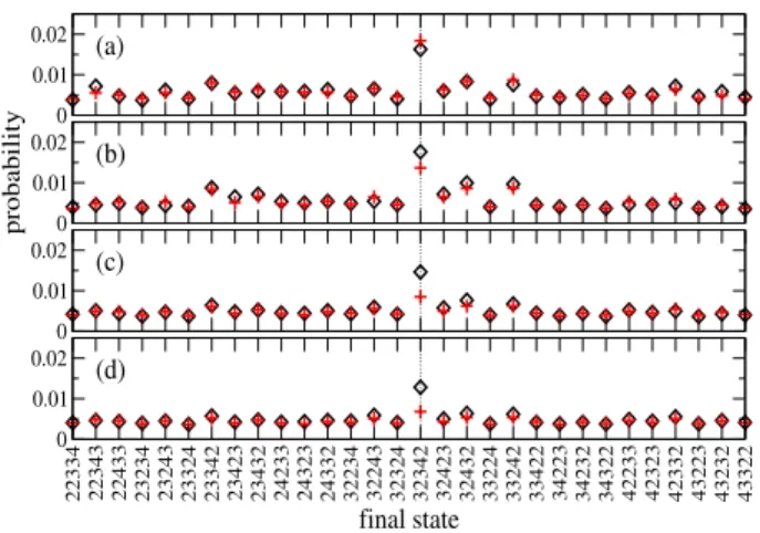
FIG. 2. (Color online) Average quantum (black diamonds) and classical (red crosses) evolution probabilities in Fock space for a Bose-Hubbard chain (L= 5, N= 14), at different evolution times (a) t = 1.5τ, (b)t = 2.5τ, (c) t = 5τ, (d) t= 10τ, withτ ≡~/J. The average was performed over an ensemble of 10³ realizations of on-site energiesα ∈[0,10J], with interaction strengthU = 4J. The probabilities are dis- played for the set of Fock states n^(f) having the same total interaction energy asn⁽ⁱ⁾= (3,2,3,2,4) (marked by the vertical dashed line). Although fort&5τ equilibration in Fock space generally sets in, the quantum backscattering probability ton^(f)=n⁽ⁱ⁾ is, in accordance with Eq. (14), systematically enhanced by about a factor two as compared to other final statesn^(f)6=n⁽ⁱ⁾and to its classical prediction.

interval 0 < _α < W. Taking advantage of the litera- ture concerned with classical equilibration and chaos for this kind of Hamiltonians [29–31], we fixed the numerical values of the free parameters U/J and W/J such that the classical phase space has a dominant chaotic component. The timet is measured in units of the inverse Rabi frequency, τ ≡ ~/J, between neighbouring sites. The quantum transition probability ¯P(n^(f),n⁽ⁱ⁾, t) is then computed with a Runge-Kutta solver, using the exact quantum propagation of the initial state in full Fock space, followed by the disorder average over the on- site energies. The classical probability ¯P^cl(n^(f),n⁽ⁱ⁾, t), on the other hand, is directly computed from Eq. (12) where, for a given random choice of the on-site energies, ψ(n⁽ⁱ⁾,θ, t) is determined by the numerical solution of theL-dimensional GPE.

In Fig. 2 we show the time dependence of ¯P and ¯P^cl as a function ofn^(f) for the BH model (3) with L= 5, N = 14 and a chain topology (i.e. the site 1 is not connected to the site L by a single hopping matrix el- ement) starting from a generically chosen initial state n⁽ⁱ⁾ = (3,2,3,2,4). After a transient time regime in which quantum and classical results resemble each other, the quantum transition probabilities clearly display, for

t & 5τ, a CBS peak at the initial state n⁽ⁱ⁾ on top of

a roughly constant background, in quantitative agreement with Eq. (14). This peak is not reproduced by the classical probabilities ruling out short-time effects or self-

(4)

223334 232334 233243 233432 242333 322334 323243 323432 332234 332342 333242 334332 343223 423233 432323 433322 0

0.004

probability

(a) ^{φ = 0}_{φ = 0.125π} φ = 0.25π φ = 0.5π φ = 0, classical

011122 012121 021211 101221 110122 111202 112102 112210 121012 121201 122110 202111 211012 211201 212110 221110

final state 0

0.004

probability

(b)

φ = 0 φ = 0.125π φ = 0.25π φ = 0.5π φ = 0, classical

FIG. 3. (Color online) Evolution probability ¯P(n^(f),n⁽ⁱ⁾, t) in Fock space averaged over random on-site energiesα∈[0, W] for a Bose-Hubbard ring of L = 6 sites (see inset). We show results for evolution times t = 10τ, hopping phases φ = 0, π/8, π/4, π/2 (black diamonds, red upper triangles, green lower triangles, blue squares) and initial statesn⁽ⁱ⁾indicated by a vertical line. In (a) we have N = 17 particles, with interaction strength U = 4J and W = 10J. The lower (more “quantum”) panel (b) hasN = 7, U = J and W = 2J. In both cases, the breaking of time-reversal invariance forφ=π/8, π/4 destroys the coherent enhancement of the backscattering probability to the initial state. In the semiclassical regime (a) the evolution probabilities globally agree with the classical prediction forφ= 0 (red crosses), while they significantly exceed the latter in the quantum regime (b).

trapping due to rare realizations of the random on-site energies as possible alternative origins of the enhancement.

Fig. 3 shows the CBS peak at t= 10τ for a BH ring (see inset) withL= 6 sites (in which a hopping matrix el- ement connects the site 1 to the siteL) in the presence of nonvanishing hopping phasesφ[see Eq. (3) which break TRI. We clearly see the suppression of the CBS peak in the absence of TRI atφ=π/8 andπ/4. Forφ=π/2, on the other hand, TRI is again established using ωα=απ in Eq. (13) and the CBS peak re-appears.

From the experimental point of view, CBS in many- body space could possibly be observed with ultracold bosonic atoms. The specific ring geometry of Fig. 3 could be realized in hexagonal (graphene) optical lattices [32].

By means of a red-detuned laser beam which is tightly focused perpendicular to the graphene lattice, an individual hexagon could be isolated from the lattice. Dis- placing the focus of the laser beam with respect to the geometric center of this hexagon would allow one to load this ring in a non-uniform manner, i.e. such that the atomic populations differ from site to site. While the ring is initially to be loaded in the deep Mott insulator regime, in which inter-site hopping along the ring is neg-

ligibly small, a sudden increase of the hopping strength at timet = 0 will make the atoms propagate along the ring. At a given final propagation time, the system would have to be quenched back to the Mott regime and the atomic populations on the individual sites would have to be measured using, e.g., high-resolution imaging techniques [33]. In order to obtain the final probability dis- tribution in Fock space with good statistical accuracy, optical disorder [34] can be used to randomly vary the on-site energies in a controlled manner, and an artifi- cial gauge field [35] could be induced in order to break TRI The lower panel of Fig. 3 displays the numerically computed Fock state probabilities on such a ring for the initial staten⁽ⁱ⁾= (1,1,2,2,1,0) [36]. It clearly displays the CBS enhancement despite the fact that this initial state is far from semiclassical (N/L'1).

Our results represent a further step in the active field of thermalization in closed many-body systems [29, 37–40].

Indeed, Eq. (14) shows that in equilibrium, even in the semiclassical limit and when the classical system displays full ergodicity, many-body quantum interference generically inhibitsquantumergodicity in equilibrium,i.e.

P¯(n^(f),n⁽ⁱ⁾, tteq)6= 1/Nacc (15) whereNacc≡ Nacc(n⁽ⁱ⁾) is the number of final Fock states that are energetically accessible ton⁽ⁱ⁾. This result, however, is not in conflict with signatures of many-body thermalization at the level of single-particle observables, like the equilibration towards uniform occupation numbers reported in Ref. [40]. As a matter of fact, Eq. (14) has an extremely small effect on such single-particle observables, as can be easily seen by calculating the averaged values ¯nα(t), which gives the expected uniform behaviour

¯

nα(t,n⁽ⁱ⁾) = (N/L) +O(1/Nacc) (16) in the regime of classical ergodicity. However, for a genuine many-body observable like the inverse participation ratio IPR(t) ∝ P

nP(n,n, t), one may obtain a strong quantum correction, IPR(t) = 2 IPR^cl(t), in the presence of TRI.

To summarize, we presented a semiclassical approach in the van Vleck-Gutzwiller spirit, using sums over interfering paths that solve a classical mean field equation, which successfully captures genuine quantum interference in interacting bosonic systems. We used this approach to predict a clear-cut quantum (and genuinely many-body) effect, namely the coherent enhancement of the return probability in Fock space. Our predictions are fully con- firmed by extensive simulations of Bose-Hubbard models with different topologies, even in the deep quantum regime where experimental observation using ultracold atoms is possible.

Acknowledgements: We thank A. Altland, T. Guhr, B. Gutkin, F. Haake, M. Oberthaler, W. Strunz, and

(5)

T. Wellens for valuable discussions. This work was fi- nancially supported by the Deutsche Forschungsgemein- schaft within the DFG Research Unit FOR760 as well as by a ULg research grant for T.E. at the Universit´e de Li`ege.

[1] A. Zeilinger, Rev. Mod. Phys.71, S288 (1999).

[2] M. Arndt, O. Nairz, J. Vos-Andreae, C. Keller, G. van der Zouw, and A. Zeilinger, Nature401, 680 (1999).

[3] J. Deiglmayr, M. Reetz-Lamour, T. Amthor, S. West- ermann, A. de Oliveira, and M. Weidem¨uller, Optics Communications264, 293 (2006).

[4] For a recent review, see E. Abrahams,50 Years of Ander- son Localization (World Scientific Publishing Company, 2010) reprinted in P. W¨olfle and D. Vollhardt, Int. J.

Mod. Phys. B24, 1526 (2010).

[5] E. Akkermans and G. Montambaux,Mesoscopic Physics of Electrons and Photons (Cambridge University Press, 2011).

[6] E. Akkermans, P. E. Wolf, and R. Maynard, Phys. Rev.

Lett.56, 1471 (1986).

[7] F. Scheffold, R. Lenke, R. Tweer, and G. Maret, Nature 398, 206 (1999).

[8] T. Schwartz, G. Bartal, S. Fishman, and M. Segev, Na- ture446, 52 (2007).

[9] A. L. Fetter and J. D. Walecka, Quantum Theory of Many-Particle Systems (Dover Publications, 2003).

[10] C. Gardiner and P. Zoller, Quantum Noise, 3rd ed.

(Springer, Berlin, 2004).

[11] A. Sinatra, C. Lobo, and Y. Castin, Phys. Rev. Lett.

87, 210404 (2001).

[12] D. Walls and G. J. Milburn,Quantum Optics (Springer, 2010).

[13] A. Polkovnikov, Annals of Physics325, 1790 (2010).

[14] F. Trimborn, D. Witthaut, and H. J. Korsch, Phys. Rev.

A79, 013608 (2009).

[15] S. Flach, D. O. Krimer, and C. Skokos, Phys. Rev. Lett.

102, 024101 (2009); Phys. Rev. Lett.102, 209903 (2009).

[16] T. Wellens and B. Gremaud, Phys. Rev. Lett. 100, 033902 (2008).

[17] M. Hartung, T. Wellens, C. A. M¨uller, K. Richter, and P. Schlagheck, Phys. Rev. Lett.101, 020603 (2008).

[18] T. Hartmann, J. Michl, C. Petitjean, T. Wellens, J.-D.

Urbina, K. Richter, and P. Schlagheck, Annals of Physics 327, 1998 (2012).

[19] J. W. Negele and H. Orland, Quantum Many-particle Systems (Advanced Books Classics) (Westview Press, 1998).

[20] See Supplementary material.

[21] W. Heisenberg, Zeitschrift f¨ur Physik33, 879 (1925).

[22] S. Mossmann and C. Jung, Phys. Rev. A 74, 033601 (2006).

[23] See M. C. Gutzwiller,Chaos in Classical and Quantum Mechanics (Springer, 1990) and references therein [24] L. Simon and W. T. Strunz, Phys. Rev. A 86, 053625

(2012).

[25] B. Juli´a-D´ıaz, T. Zibold, M. K. Oberthaler, M. Mel´e- Messeguer, J. Martorell, and A. Polls, Phys. Rev. A86, 023615 (2012).

[26] In order to derive the second line of Eq. (12), we use the

classical identity θ^(i/f) = ∓∂R(n^(f),n⁽ⁱ⁾, t)/∂n^(i/f) (mi- nus forθ⁽ⁱ⁾ and plus forθ^(f)) for each trajectoryγ.

[27] In the Truncated Wigner approach, one propagates, instead of a single trajectory, full initial manifolds in phase space (n, θ) representing the initial quantum state.

For the case of the transition probability, the manifold δ(n−n⁽ⁱ⁾) is classically propagated and projected at time toverδ(n−n^(f)), thus giving ¯P^cl.

[28] Loop corrections [41] can be shown to identically vanish in this case.

[29] A. C. Cassidy, D. Mason, V. Dunjko, and M. Olshanii, Phys. Rev. Lett.102, 025302 (2009).

[30] M. Lubasch, Quantum chaos and entanglement in the Bose-Hubbard model, Master’s thesis, Ruprecht-Karls- Universit¨at Heidelberg (2009).

[31] M. Hiller, T. Kottos, and T. Geisel, Phys. Rev. A79, 023621 (2009).

[32] L. Tarruell, D. Greif, T. Uehlinger, G. Jotzu, and T. Esslinger, Nature483, 302 (2012).

[33] W. Bakr, J. Gillen, A. Peng, S. F¨olling, and M. Greiner, Nature 462, 74 (2009); J. Sherson, C. Weitenberg, M. Endres, M. Cheneau, I. Bloch, and S. Kuhr, Nature 467, 68 (2010).

[34] J. E. Lye, L. Fallani, M. Modugno, D. S. Wiersma, C. Fort, and M. Inguscio, Phys. Rev. Lett. 95, 070401 (2005).

[35] Y.-J. Lin, R. Compton, K. Jimenez-Garc´ıa, J. Porto, and I. Spielman, Nature462, 628 (2009).

[36] In order to prevent three-body losses, it is preferrable to avoid populations of more than two atoms per site.

[37] M. Gring, M. Kuhnert, T. Langen, T. Kitagawa, B. Rauer, M. Schreitl, I. Mazets, D. A. Smith, E. Demler, and J. Schmiedmayer, Science337, 1318 (2012).

[38] T. Langen, R. Geiger, M. Kuhnert, B. Rauer, and J. Schmiedmayer, “Local emergence of thermal corre- lations in an isolated quantum many-body system,”

(2013), preprint, arXiv:1305.3708.

[39] T. Geiger, T. Wellens, and A. Buchleitner, Phys. Rev.

Lett.109, 030601 (2012).

[40] S. Trotzky, Y.-A. Chen, A. Flesch, I. McCulloch, U. Schollw¨ock, J. Eisert, and I. Bloch, Nature Physics 8, 325 (2012).

[41] K. Richter and M. Sieber, Phys. Rev. Lett.89, 206801 (2002); D. Waltner, Semiclassical Approach to Meso- scopic Systems, Springer Tracts in Modern Physics, Vol.

245 (Springer, Berlin, 2012).

(6)

Supplementary material for

“Coherent Backscattering in Fock Space:

a Signature of Quantum Many-Body Interference in Interacting Bosonic Systems”

Thomas Engl,¹ Julien Dujardin,² Arturo Arg¨uelles,² Peter Schlagheck,² Klaus Richter,¹ and Juan Diego Urbina¹

1Institut f¨ur Theoretische Physik, Universit¨at Regensburg, D-93040 Regensburg, Germany

2Département de Physique, Université de Liège, 4000 Liège, Belgium

The semiclassical propagator cannot be directly obtained in Fock state representation, since the Fock states form a discrete basis rather than a continuous one as re- quired by the path integral formalism. To solve this problem, we first derive a semiclassical propagator in quadrature representation and then project the result on Fock states.

The quadrature eigenstates |qi ≡ |q1, . . . , q_Li and

|pi ≡ |p1, . . . , p_Liare defined as the eigenstates of linear hermitian combinations of the creation and annihilation operators associated with the single-particle orbitals χ_α (α= 1, . . . , L),i.e.,

b ˆaα+ ˆa^†_α

|qi=qα|qi (17)

−ib ˆaα−aˆ^†_α

|pi=pα|pi, (18) with an arbitrary but fixed scale b. These quadrature eigenstates obey the resolutions of unity

Z

d^Lq|qihq|= ˆ1 = Z

d^Lp|pihp| (19)

and their overlap matrix elements are given by

hq|q⁰i=δ(q−q⁰) , (20) hp|p⁰i=δ(p−p⁰) , (21)

hq|pi= 1 2b√

πexp ip·q

2b²

. (22)

Following the usual steps to derive the Feynman propagator (i.e., splitting up the exponential into a product ofN exponentials, inserting unity operators in terms of ˆ

q and ˆp between each pair of exponentials, and taking the limitN → ∞), we find for the Hamiltonian

Hˆ =X

αβ

h_αβˆa^†_αˆa_β+1 2

X

αβµσ

V_αβµσâ^†_αâ_βâ^†_µâ_σ (23)

[see Eq. (2) in the Letter] a path integral representation of the propagator in quadrature representation as

K

q^(f),q⁽ⁱ⁾, t

= lim

N→∞

Z

dq⁽¹⁾· · · Z

dq^(N⁻¹⁾

Z dp⁽¹⁾ 4πb² · · ·

Z dp^(N⁾ 4πb²

N

Y

k=1

exp

"

i

2b²p^(k)·

q^(k)−q^(k−1)

−iτ

~

L

X

α,β=1

h_αβ(ψ_α^(k))^∗ψ^(k)_β − iτ 2~

L

X

α,βµ,σ=1

V_αβµσ(ψ^(k)_α )^∗(ψ_µ^(k))^∗ψ^(k)_β ψ^(k)_σ

#

, (24)

with 2bψ^(k)≡q^(k−1)+ ip^(k), 2b(ψ^(k))^∗≡q^(k−1)−ip^(k), and τ ≡ t/N. Calculating the integrals in stationary phase approximation and finally taking the limitN → ∞ yields the van-Vleck-Gutzwiller propagator

K

q^(f),q⁽ⁱ⁾, t

= 1

(−2πi~)^L/2

×X

γ

s

det ∂²Rγ

∂q⁽ⁱ⁾∂q^(f)e^iR^γ^/^~ (25) where the sum runs over all possible classical trajectories

defined by the equation of motion

i~∂ψα(s)

∂s =

L

X

β=1

hαβψβ(s)

+

L

X

β,µ,σ=1

Vαβµσψ_µ^∗(s)ψβ(s)ψσ(s) (26)

and the boundary conditions 2bRe[ψ(0)] = q⁽ⁱ⁾ and 2bRe[ψ(t)] =q^(f). R_γ is the classical action given by

R_γ

q^(f),q⁽ⁱ⁾, t

=

t

Z

0

ds (

~

2b²p(s)·q(s)˙ −

L

X

α,β=1

h_αβψ^∗_α(s)ψ_β(s)−1 2

L

X

α,β,µ,σ=1

V_αβµσψ^∗_α(s)ψ_β(s)ψ_µ^∗(s)ψ_σ(s) )

(27)

(7)

withq(s)≡2bRe[ψ(s)] andp(s)≡2bIm[ψ(s)] evaluated along the trajectoryγ.

We now want to project the result onto Fock states.

To this end, we need the overlap

hn|qi= 1 p2ⁿn!√

2πb exp

−q² 4b²

Hn

q

√2b

(28)

of a quadrature eigenstate|qi with a Fock state|nias- sociated with an individual single-particle orbital. For largen, we can employ the WKB approximation for the Hermite polynomialsHn, which yields

hn|qi '

p2/π (4b²n−q²)^1/4

×cosh q 4b²

p4b²(n+ 1/2)−q²i

(29)

within the oscillatory region |q| ≤ 2b√

n. Since hn|qi decreases exponentially for larger values of |q|, we can restrict the integration necessary for the projection onto Fock states to the oscillatory region|q| ≤2b√

n.

With this restriction, we substituteqα^(i/f)7→θα^(i/f)(α∈ {1, . . . , L}) withθ^(i/f)α ∈[−π, π] defined through

q⁽ⁱ⁾₁ ≡2b q

n⁽ⁱ⁾₁ + 1/2 cos θ⁽ⁱ⁾₁

, (30)

q^(f)₁ ≡2b q

n^(f)₁ + 1/2 cos

θ^(f)₁ +θ₁⁽ⁱ⁾

, (31)

as well as

q_α^(i/f)≡2b q

n^(i/f)α + 1/2 cos

θ_α^(i/f)+θ⁽ⁱ⁾₁

(32)

for α = 2, . . . , L. The integrations over θ^(f)₁ , . . . , θ_L^(f), θ⁽ⁱ⁾₂ , . . . , θ_L⁽ⁱ⁾ can now be performed in

stationary phase approximation. This selects trajectories that satisfy

ψ₁(t) = q

n^(f)₁ + 1/2 expn i

θ^(f)₁ +θ⁽ⁱ⁾₁ o

, (33)

as well as ψα(0) =

q

n⁽ⁱ⁾α + 1/2 expn i

θ^(f)_α +θ₁⁽ⁱ⁾o

(34) ψα(t) =

q

n^(f)α + 1/2 expn i

θ^(f)_α +θ₁⁽ⁱ⁾o

(35) forα= 2, . . . , L. Since the classical equations of motion preserve|ψ1(t)|²+. . .+|ψL(t)|², these stationary phase conditions already imply|ψ1(0)|² =n⁽ⁱ⁾₁ + 1/2 provided the final state

n^(f)i contains as many particles as the initial state

n⁽ⁱ⁾i. Due to theU(1) gauge symmetry, a variation of the global phase θ⁽ⁱ⁾₁ will trivially give rise to another solution ψ⁰ = ψexp(θ₁⁽ⁱ⁾) that exhibits the same initial and final populations as ψ. Therefore, one cannot solve the integral over θ⁽ⁱ⁾₁ in stationary phase approximation, but needs to do it exactly, which yields an additional factor 2π.

The propagator in Fock space then finally reads K

n^(f),n⁽ⁱ⁾, t

= 1

(−2πi~)^(L−1)/2

×X

γ

r

det⁰ ∂²Rγ

∂n⁽ⁱ⁾∂n^(f)e^iR^γ^/^~, (36) whereγ indexes all classical trajectories that satisfy the boundary conditions|ψα(0)|²=n⁽ⁱ⁾α + 1/2 and|ψα(t)|²= n^(f)α + 1/2 for α = 1, . . . , L with the global phase θ₁⁽ⁱ⁾ being fixed through the choice ψ₁(0) = [n⁽ⁱ⁾₁ + 1/2]^1/2. The prime at the determinant

det⁰ ∂²Rγ

∂n⁽ⁱ⁾∂n^(f) ≡det ∂²Rγ

∂n⁽ⁱ⁾α∂n^(f)_β

!

α,β=2,...,L

(37)

indicates that it is taken with respect to the matrix obtained by skipping the derivatives with respect to the first components.