Evaluation Strategies in Labor Economics – An Application to Post-Secondary Education

(1)

Evaluation Strategies in Labor Economics – An Application to

Post-Secondary Education

Inaugural-Dissertation zur Erlangung

der W¨ urde eines Doktors der Wirtschaftswissenschaften der Wirtschaftswissenschaftlichen Fakult¨ at

der Ruprecht-Karls-Universit¨ at Heidelberg

vorgelegt von Boris Augurzky

aus Heilbronn

Heidelberg, Oktober 2000

(2)

List of Tables

2.1 Distribution of Estimated Propensity and Index Score. . . . 20 2.2 Estimated Eﬀects. Matching on the p.score, Within caliper:

p.score. . . . 26 2.3 Estimated Eﬀects. Matching on the p.score, Within caliper: Ma-

halanobis. . . . 27 2.4 Estimated Eﬀects. Matching on the index, Within caliper: index. 28 2.5 Estimated Eﬀects. Matching on the index, Within caliper: Ma-

halanobis. . . . 29 2.6 Balance of Covariates, Aggregate Measures. . . . 30 2.7 Probit Estimation Results. . . . 38 2.8 Balance of Covariates: Matching on the p.score, Within calipers:

p.score. . . . 43 2.9 Balance of Covariates: Matching on the p.score, Within calipers:

Mahalanobis. . . . 44 2.10 Balance of Covariates: Matching on the index, Within calipers:

index. . . . 45 2.11 Balance of Covariates: Matching on the index, Within calipers:

Mahalanobis. . . . 46

iv

(5)

v

3.1 The Simulation Setup. . . . 58

3.2 Distribution of Treated and Untreated Individuals. . . . 60

3.3 Speciﬁcation of Caliper Width ε. . . . 61

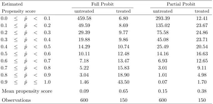
3.4 Basic Model, Full Probit. . . . 66

3.5 Basic Model, Partial Probit. . . . 67

3.6 Mean Ranks. . . . 71

3.7 Alternative Model. . . . 72

4.1 Distribution of the Estimated Index Score. . . . 87

4.2 Balance of Covariates, AA. . . . 92

4.3 Balance of Covariates, BA. . . . 93

4.4 Balance of Covariates, MA. . . . 94

4.5 Treatment Eﬀects, Men, AA, Narrow Probit Model. . . . 97

4.6 Treatment Eﬀects, Men, AA, Broad Probit Model. . . . 98

4.7 Treatment Eﬀects, Women, AA, Narrow Probit Model. . . . 100

4.8 Treatment Eﬀects, Women, AA, Broad Probit Model. . . . 101

4.9 Treatment Eﬀects, Men, BA, Narrow Probit Model. . . . 103

4.10 Treatment Eﬀects, Men, BA, Broad Probit Model. . . . 104

4.11 Treatment Eﬀects, Women, BA, Narrow Probit Model. . . . 107

4.12 Treatment Eﬀects, Women, BA, Broad Probit Model. . . . 108

4.13 Probit Estimation Results. . . . 114

4.14 Treatment Eﬀects, Men, MA. . . . 117

4.15 Treatment Eﬀects, Women, MA. . . . 118

(6)

vi

5.1 Return to Education for Men According to Weiss. . . . 125

5.2 Return to Education for Men According to Park. . . . 126

5.3 Return to Education According to Altonji & Dunn. . . . 127

5.4 Description of Variables. . . . 129

5.5 Local Returns to Education, Men. . . . 131

5.6 Local Returns to Education, Women. . . . 132

5.7 Estimation Results for Men. . . . 134

5.8 Estimation Results for Women. . . . 135

5.9 Detailed Regression Results. . . . 143

5.10 Observations Per Education Cell. . . . 144

5.11 Men, Potential Experience. . . . 145

5.12 Women, Potential Experience. . . . 146

6.1 Variables and Parameters. . . . 157

6.2 Estimation Results, Selection at the Individual Level.. . . 162

6.3 Estimation Results, Selection at the Group Level. . . . 167

6.4 IV Versus Experiment. . . . 169

(7)

List of Figures

2.1 Illustration of the Evaluation Procedure. . . . 23

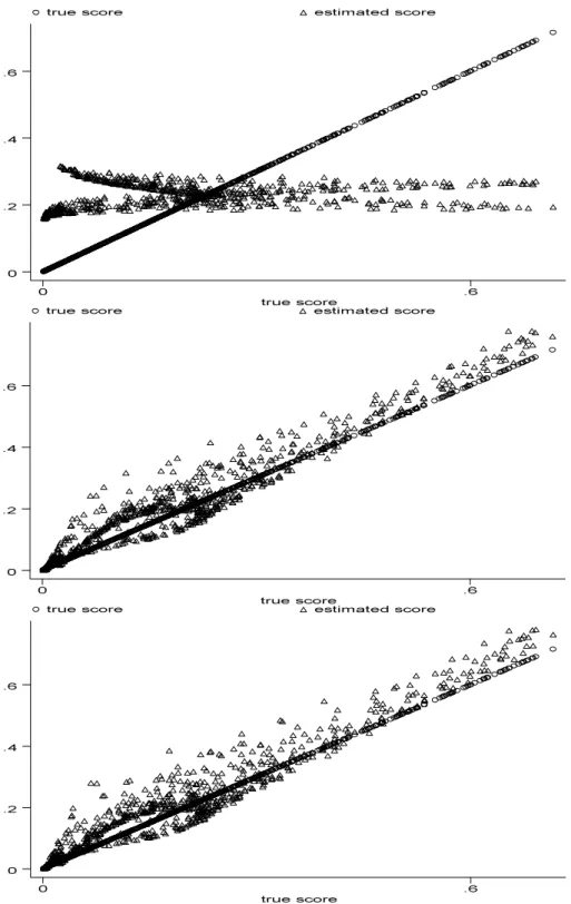
3.1 Basic Model, Full Probit and Partial Probit . . . 65 3.2 Alternative Model, Partial Probit With and Without Higher Or-

der Terms . . . 70

4.1 Illustration of the Evaluation Procedure. . . . 89

vii

(8)

Chapter 1 Introduction and Overview

Identifying causal relationships is of central concern in many applied economic research.

For example, political groups might be interested in how union membership affects labor market outcomes of union members. The government might want to know how certain active labor market programs help improve participants’ labor market status. Frequently, for the sake of evaluation of such programs, candidate causal variables are simply compared with their supposed effects. However, a simple bivariate comparison might generally lead to misinterpretations and wrong conclusions. Most likely, there might be other – so-called confounding – forces determining both the supposed cause and its effect. For example, participants in an active labor market program might systematically differ from non- participants, say, they have higher motivation or higher program-specific skills, such that they would be more successful in the labor market anyway, even without the program.

Thus, the association of participation and success in the labor market might wrongly be interpreted as a causal relationship. Applied econometric research attempts to take account of confounding background variables by multivariate estimation techniques such as the classical linear multivariate regression approach.

Recently, the econometric literature has been incorporating a new alternative statistical technique which does not need to rely intensively on parametric or functional form assumptions (see Heckman, LaLonde & Smith, 1999, and Angrist & Krueger, 1999). Rather, this technique is based on directly matching individuals who are equal in

(9)

Chapter 1: Introduction 2

all observable respects with the only exception that one individual has experienced the impact of a potentially causal variable while the other has not. Their difference in the outcome variable under scrutiny will then be attributable to the effect of the interven- tion. The idea of matching originates in the randomized controlled trial (RCT). In an RCT with binary causal variable, units are randomly assigned to one of two states, either the treatment or the control state. Then, the treatment effect is estimated by taking the difference between the mean outcome of treated and control units. The estimate is unbiased since the randomization property of the experiment – if implemented appropriately – ensures that, on average, all covariates of treated and control units – be they observed or unobserved – are balanced. In contrast to an RCT, in an observational study treated and untreated units may differ considerably because of their being self-selected into the treatment state in lieu of being selected by an exogenous random mechanism.

Matching aims at removing systematic imbalance of covariates in an observational study by selecting controls from the untreated group, the control reservoir, who are “similar” to treated units in all relevant variables. In other words, it aims at constructing an artificial control group. Of course, imbalance in unobservable characteristics cannot be remedied. Insofar, both matching and the classical linear regression model control for observable confounding variables. Yet, the difference is that the first technique is non- parametric while the latter interpolates linearly when there are no perfectly equal units.

However, note that even a saturated linear model would not necessarily identify the same parameter as matching if heterogeneity in the effect was present (see Angrist, 1998 or Angrist & Krueger, 1999). This is because OLS and matching impose different weighting schemes when averaging over individual effects.

If the relevant variables are of high dimension exact matching in a ﬁnite sample is, in all likelihood, impossible. As an alternative, Rosenbaum & Rubin (1983) suggest in their seminal paper to match on the one-dimensional probability of participation in the treatment, the propensity score. They show that matching on the propensity score is a valid approach whenever matching on all covariates is valid. However, since the propensity score is unknown, further problems might arise in its estimation. For example, it is often unclear how to specify the selection equation, which variables to include in

(10)

the estimation, and how to deﬁne a propensity score distance. Furthermore, in case of parametric binary choice models – probit or logit – the question arises whether to match on the estimated index, i.e. the probits or logits, that is linear in the covariates or to match on the estimated propensity score that, in order to be located in the unit interval, depends on the covariates in a nonlinear fashion.

In this thesis the matching approach is used to evaluate postsecondary education and to contrast estimation results with conventional ordinary least squares estimation. To this end, data are drawn from the National Longitudinal Survey of Youth 1979 (NLSY), an American panel data set that started in 1979, comprising young individuals aged between 14 and 22 who have been re-interviewed annually until 1994 and biennially thereafter. In terms of the matching methodology, postsecondary education constitutes the treatment while the control reservoir is made up of individuals having a high school diploma only.

All empirical chapters of this thesis will use these data.

It turns out that selection into college, especially into four-year colleges, is extraordinar- ily strong. Observable variables such as ability test scores and socio-economic background variables are essential determinants aﬀecting the decision to take up a college education.

Unfortunately, matching treated and untreated units in such a case is no easy matter. For instance, in the extreme case, if selection were perfectly predictable, matching would be impossible because there would be no unit in the control reservoir having the same characteristics as any treated. Note that also a linear model interpolating the extremes would not be promising either. Consequently, pair matching, i.e. matching exactly one treated and one untreated, as frequently pursued in applied work to evaluate active labor market programs (see e.g. Lechner, 1999), might be inappropriate in the schooling example. It would have to drop great a number of treated units at the high end of the propensity score scale and, thus, it would produce matched pairs which are not anymore representa- tive of the whole treated population. Hence, if the treatment eﬀect is heterogeneous pair matching estimates might be severely biased.

In order to keep as many treated units as possible, one control should be matched to more than one treated person, something which is often referred to as matching with re-

(11)

placement. Dehejia & Wahba(1998) suggest an algorithm which follows this approach.

Usually, however, this algorithm lacks some optimality criterion in that it does not necessarily achieve to minimize the overall distance between treated and control units. What is more, several controls could also be matched to one treated unit to increase statistical precision. In the end, the full sample might be stratiﬁed into small strata consisting of either one treated and one or more controls or one control and more than one treated unit.

Rosenbaum (1991) suggests an optimal full matching algorithm which not only matches all units in the sample but which also manages to minimize the total distance between treated and controls. In general, however, exact matches on the propensity score are not possible and a certain small distance between the matched treated and the control has to be accepted. Greedy algorithms address this issue by matching a randomly chosen treated unit to the closest untreated available who will then be removed from the sample. By contrast, the optimal algorithm is apt to ﬁnd the overall minimum distance by reconsidering and possibly rearranging already matched units.

Chapter 2 examines several steps in the practical implementation of the method of matching. Typically, the applied researcher has to make decisions on how to adapt certain parameters in the matching algorithm. In contrast to the simulation study of Gu

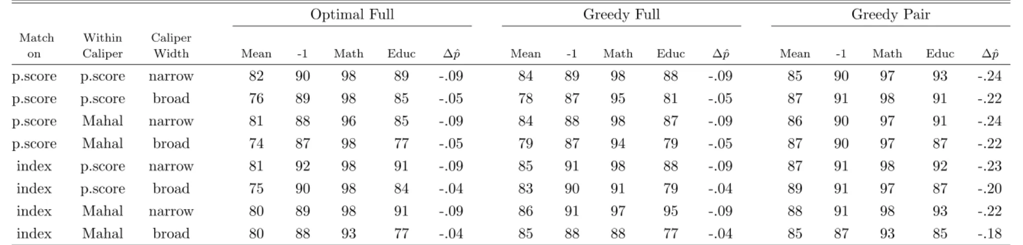
& Rosenbaum (1993), this chapter performs a sensitivity analysis with data from the NLSY. First, it analyses whether matching on the propensity score or on the linear index is to be preferred. Second, it suggests to use a so-called propensity score caliper approach which ensures that the distance between the treated and control unit does not exceed a certain pre-specified range. Otherwise, arbitrarily large distances might occur. A broad and a narrow caliper width are set against. Third, the question arises how to define distance within calipers. The literature suggests to either use the propensity score distance or the Mahalanobis metric, both of which will be investigated. Fourth, three matching algorithms are compared: optimal full, a greedy full, and a greedy pair matching. Fifth, suitable stratum weighting schemes are built to identify the mean effect of treatment on the treated and the mean effect on a randomly assigned person. The results will be discussed with respect to three measures of success: balance of covariates after matching,

(12)

variance of the matching estimates, and how systematic treated units are discarded by the algorithms.

Sensitivity of the decision parameters as to the estimated treatment eﬀects appears to be rather modest. Systematic variation in the estimates caused by variation of the distance measures between treated and untreated units or by altering matching algorithms is negligible and statistically insigniﬁcant. Moreover, roughly 80% of the initial bias in the observable covariates is removed by full matching algorithms and 87% by pair matching.

Yet, mean propensity scores of pair-matched treated individuals are markedly lower than in the original treatment group before matching. If high-propensity score individuals experience a higher eﬀect of their education pair matching estimates are expected to be biased.

Alas, heterogeneity is too weak to unanimously favor full matching since its disadvantages clearly emerge. Full matching estimates are accompanied by relatively large standard errors because a full stratiﬁcation is far from being as uniform as pair matching.

For example, the more strata consist of a large number of treated units sharing only one control the higher standard errors of the estimated mean effect on the treated individual are. It turns out that the specific greedy full algorithm as implemented in this thesis achieves a more uniform stratification than the optimal one. Notwithstanding, in order to attain a more uniform stratification, greedy algorithms can always be replaced by a suitable optimal one when restrictions on the size of the strata are incorporated in the optimization process. Therefore, greedy algorithms should be abandoned. Furthermore, matching on the linear index score turns out to better discriminate between units at the low end of the propensity score scale. As a result, it drops many low-score untreated individuals who would almost all be used in matching on the propensity score.

Chapter 3 is dedicated to specific problems that might arise under strong selection into college as in Chapter 2. If treatment effects are heterogeneous and selection into treatment is exceptionally strong, pair matching is an efficient evaluation strategy. In the heterogeneous case, it is unclear which matching method to prefer. This chapter, however, suggests to concentrate less on the choice of method but, alternatively, to carefully recon-

(13)

sider the selection equation. Some variables might be strong determinants of the selection but exhibit a rather modest impact on the outcome. If they are omitted randomness of the selection process increases or, in other words, some observable self-selection is left to stochastic noise. This will result in a smaller propensity score diﬀerence between treatment and comparison group and, consequently, matching will become easier. Only the relevant variables which rule both the selectionand the outcome have to be balanced.

On the other hand, a consistent estimation of the propensity score might make it necessary to include into the selection equation all the variables that rule the selection process even if they do not determine the outcome. Many applied research emphasizes the importance of consistent estimation of the selection equation. For instance,Lechner (1999, 2000) performs and recommends several speciﬁcation tests to examine whether a probit model is adequate for describing the selection decision. Heckman, Ichimura &

Todd (1997: section 8) choose the predictor variables to maximize the within-sample correct prediction rates of participation. Although a selection process well understood might in itself be an important contribution, it is not the main objective of propensity score matching envisaging to identify the mean eﬀect of treatment. What is to be achieved by propensity score matching is balance of the relevant covariates in order to eliminate selection bias, even if the propensity score is inconsistently estimated. Obviously, there is a trade-oﬀ between feasible matching on the one hand and consistent estimation of the propensity score on the other.

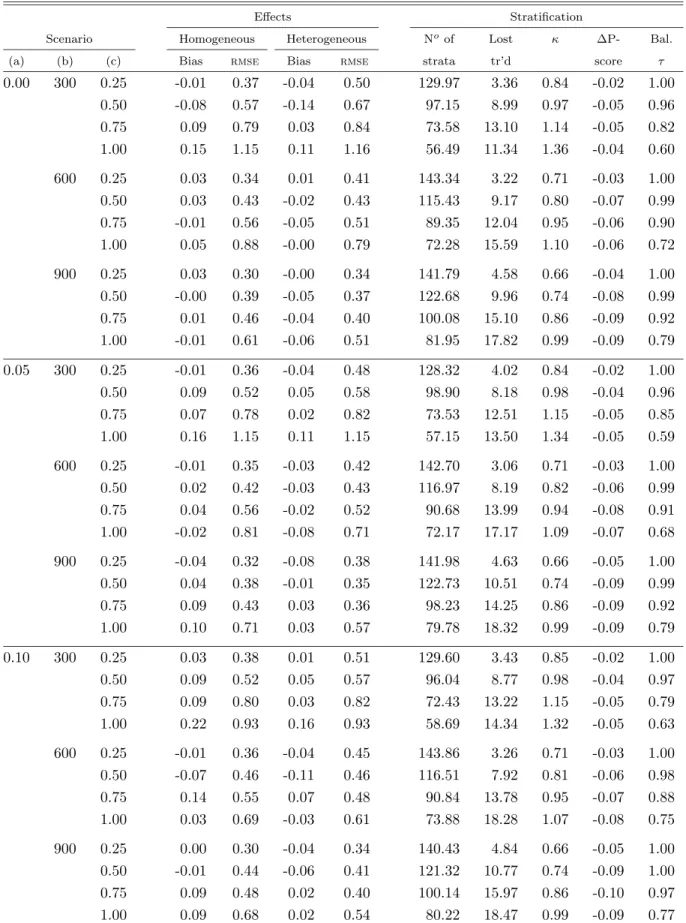
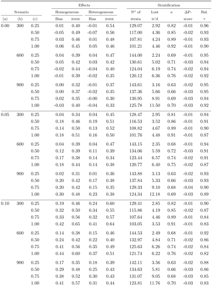
To assess this trade-off Chapter 3 performs a simulation study. It turns out that even when matching builds on quite inconsistent propensity score estimates, estimation results of the mean effect of treatment can still be superior, in terms of the mean squared error, to results produced by a consistent propensity score estimation which might separate treated and untreated units too successfully. The findings of this simulation study recommend to only include variables into the selection equation that are highly significant. Variables with low significance levels are obvious candidates for exclusion, even if they might play a role in the outcome equation. Furthermore, if established research suggests that certain variables are irrelevant to the outcome under study, they should solely be included if there are other strong reasons for doing so. In sum, the main criterion to judge the success of

(14)

matching is how well it balances the relevant covariates. This aim is more likely to be obtained if self-selection is weak or the control reservoir is large.

Chapter 4 concentrates on the evaluation of post-secondary education by the method of matching incorporating the findings of the previous two chapters. A somewhat different concept of return to education is introduced, namely the effect of college education on earnings, which takes account of the effect of education on labor market experience, as well. Its primary aim is estimation of the effect of the associate’s, the bachelor’s, and graduate degrees on hourly wages for both men and women during the first ten years after they have finished their college education. Moreover, heterogeneity in the effect ruled by family background and inherent ability will be considered. The results are compared to conventional OLS estimation which allows (i) to verify the linear specification of the earnings equation and (ii) to bring out the determinants why matching and OLS estimates differ. Indeed, there is evidence that matching and OLS deviate particularly when heterogeneity in the effect is substantial. For men, the effect of college education on wages seems to depend significantly on ability and parents’ education, while, for women, estimates do not support such clear heterogeneity. At the same time, matching and OLS estimates differ less for women than for men.

Basically, the empirical results are along the lines of the existing literature. Estimates of the effect of college education are larger for women. Individuals who obtained their degree more recently experience a higher effect, i.e. there is evidence in favor of a general increase. Moreover, the effect seems to grow gradually over the first ten years after leaving college. Yet, this growth cannot be attributed to a positive interaction between experience and education but partly to a faster accumulation of labor market experience on the part of college graduates.

Apart from evaluating the eﬀects by the method of matching, Chapter 5 examines the functional form assumption of the typical Mincerian human capital earnings equation.

A formal framework recently proposed by Card (1995, 1999) is used to take account of endogeneity of the schooling decision. If the return to education depends positively on inherent earnings abilities, individuals with higher abilities tend to opt for more schooling.

(15)

If ability is itself rewarded in the labor market but is not controlled for in regression analyses, coeﬃcient estimates of the return to schooling might be upward biased. Griliches (1977) discusses this classical ability bias. However, this chapter shows that not con- trolling for ability might additionally bias the estimated functional form of the earnings equation. Indeed, this bias leads to returns to education that increase with years of schooling acquired, thus rejecting constant returns as generally assumed in the literature (Becker, 1967,Mincer, 1974). Other empirical studies also implicitly report increasing marginal returns to schooling as years of education rise. This suggests that postsecondary education might work as some magic potion.

However, these ﬁndings seem to be prompted by endogeneity of schooling as a result of the optimization behavior. Explicit control for ability, especially for an interaction between ability and schooling, shows that, in fact, the return to education diminishes as more schooling is acquired, especially for men. In particular, the results show that the interaction term is mostly statistically signiﬁcant, i.e. that heterogeneity in the returns is substantial.

Finally, Chapter 6 treats self-selection on unobservables and compares possible solu- tions to problems raised by this additional dimension in a numerical simulation study.

While it is straightforward to tackle selection on observables, selection on unobservables provides a serious intellectual challenge. Researchers have proposed several alternative strategies to overcome thisidentiﬁcation problem, b y invokinga prioriinformation on the process of selection into treatment in an observational study (Heckman & Robb, 1985, Angrist & Krueger, 1999) or by designing an appropriate randomized experiment.

In the natural sciences, the RCT has become the method of choice for the evaluation of interventions.

While emphasis in methodological work is on the individual level, practical applications frequently concern the case of group-level or community-based interventions. Implemen- tation of policy measures at the community level is often a matter of necessity. Moreover, analysts might choose a community-level approach to evaluation for reasons of costs.

Nothing seems more natural as a methodological approach to the evaluation of these in-

(16)

terventions than the translation of the RCT paradigm to the community level. Objects of randomized assignment into treatment and control samples are then entire communities. The possible correlation of outcomes within communities, clusters, or groups might seriously distort conclusions regarding the statistical precision of the results.

Although one might be able to collect data on sizeable numbers of individuals within each community participating in the study, the number of communities is typically limited.

Thus, while group-randomized experiments produce unbiased estimates it is difficult to enhance precision. Observational studies, by contrast, typically include a respectable number of communities, yet, they might suffer from the selection problem. Possibly, a biased but more precise estimate from an observational study may yield a lower mean squared error than the corresponding estimate of program impact from a group-randomized experiment. In other words, there might be a serious trade-off to consider in the choice of the evaluation strategy.

Chapter 6 investigates the potential and the limits of experimental and non- experimental approaches to the evaluation problem. In particular, it contrasts the use of instrumental variables as a quasi-experimental technique against the particular background of community-based interventions. In the simulations, trade-oﬀ between bias and precision is emphasized by imposing a smaller number of communities in a randomized experiment, and by allowing for a correspondingly larger number of communities in all cases where selection into the program is not controlled by the analyst.

Obviously, standard estimators perform well as long as more or less restrictive assumptions on the selection process are satisﬁed. The randomized experiment – appropriately implemented – always performs well without imposing strong assumptions. However, its small sample size involves disadvantages, especially at group level. Instrumental variable estimation may be a helpful device to circumvent the small sample problem and may open the ﬁeld for less costly large scale observational studies, provided that a suitable instrument is available. The simulation results suggest that correlations between instrument and endogenous treatment indicator of around 0.3 to 0.4 can be considered to make up a good instrument if the observational study comprises ten times more observations than a

(17)

randomized experiment.

IV estimation yields inconsistent estimates, though, if treatment effects are heterogeneous and individuals or groups decide whether to undergo treatment upon their true effects. In this case, IV identifies the mean effect of treatment on compliers, the so-called local average treatment effect (LATE), see e.g. Angrist, Imbens & Rubin (1996). In case of a binary instrument, for example, LATE identifies the mean effect of those individuals who opt for participation in accordance with the value of their instrument. That is, they participate if the instrument takes the value 1 and they do not if it is 0. Note that this parameter might also be policy relevant, for instance, in answering the question whether to install additional treatment sites or not, when proximity to treatment site is a valid instrument.

(18)

Chapter 2 Matching the Extremes – A

Sensitivity Analysis Based on Real Data

May 1999/October 2000

Abstract. This chapter uses observational data to estimate the eﬀect of a bachelor’s degree on earnings for men by the method of matching. The data exhibit an extraor- dinarily large bias in terms of observable confounding variables between treatment and comparison group. Therefore, an appropriate implementation of the matching technique is crucial. Usually, several ad hoc decisions have to be made in advance, e.g. decisions on which distance measure or which matching algorithm to use. Sensitivity of the estimation results with respect to some decisions is investigated. In particular, optimal full matching, a greedy full matching, and a greedy pair matching are compared. Furthermore, a simple extension permitting heterogeneous treatment eﬀects is suggested.

(19)

Chapter 2: Matching the Extremes 12

2.1 Introduction

Recently, the statistical technique of matching has found widespread attention in econo- metrics to evaluate effects of policy interventions or welfare programs (Heckman, Ichimura & Todd, 1997, Kluve, Lehmann & Schmidt, 1999, or Lechner, 1999, 2000), or to estimate labor market impacts of military service (Angrist, 1998). Heck- man, LaLonde & Smith(1999) provide a comprehensive overview. The technique rests on matching untreated individuals to treated ones with the same (observable) characteristics, thus generating an artificial counterfactual of the treatment group. In effect, this approach attempts at mimicking a randomized experiment using data from an observational study to estimate the mean effect of treatment.

Unlike ordinary least squares estimation (OLS) matching as a non-parametric technique need not rely on functional form or distributional assumptions. What is more, in contrast with OLS, if the treatment effect is heterogeneous the estimated mean effect of treatment – a weighted average of individual effects – builds on a more appropriate weighting scheme than OLS. Angrist & Krueger (1999) or Angrist (1998) show how in case of heterogeneous treatment effects a saturated linear model estimated by OLS weights the individual effects by the individual variances of the treatment indicator. In contrast, matching weights the individual effects by the probability to participate in treatment which is considered a more appropriate weighting scheme.

Often, applied research using propensity score matching has to make many ad hoc decisions at various steps of the implementation. For example, decisions have to be made on the concrete deﬁnition of a distance measure between treated and untreated units and on which matching algorithm and weighting scheme to use. In an extensive simulation study, Gu & Rosenbaum (1993) examine several alternatives. This chapter uses real observational data from the National Longitudinal Survey of Youth 1979 to investigate sensitivity of the estimation results with respect to some crucial decisions, speciﬁcally decisions on the distance measure and the algorithm to be employed, and, furthermore, on which propensity score estimate to match on.

(20)

The empirical example evaluates college education by estimating the eﬀect of the bachelor’s degree for men during the ﬁrst ten years after graduation from college.¹ It turns out that selection into college is extremely strong such that treatment and comparison group are quite distinct. Hence, matching adequate individuals can be expected to be a serious challenge. As a result, the matching algorithm should take account of potential pitfalls which is why three matching algorithms will be explored: optimal full matching proposed by Rosenbaum (1991), agreedy full matching, and a greedy pair matching.

Pair matching produces a stratification composed of non-overlapping pairs of treated and control units. It drops all untreated individuals who are not matched which might reduce efficiency. More importantly, given a certain distance measure some treated might not find a control which would give rise to biased estimates if the loss of treated individuals were systematic and the treatment effect were heterogeneous. In this case, afullmatching procedure which uses all treated and all untreated units in the sample might be preferred.

In a full matching, one control may be matched to more than one treated person and, likewise, one treated may also be matched to numerous controls. The latter event will occur particularly at the low end of the propensity score scale while the first event will mainly happen at the high end. What is more, in a natural way, full matching provides weighting schemes that permit estimation of the mean effect of treatment on the treated as well as the mean effect on a randomly assigned person.

Dehejia & Wahba (1998) suggest a solution where controls are allowed to be used more than once in a matching algorithm with replacement. However, their strategy generally produces overlapping strata, i.e. certain individuals might be member of more than one stratum. This makes statistical inference more difficult due to dependencies across strata. In contrast, this study adopts the optimal full stratification strategy which produces non-overlapping strata and achieves to effectively minimize the total distance between treated and untreated units. It will be contrasted to a greedy full matching.

“Greedy” means that the algorithm does not necessarily attain the minimum. In addi- tion, the framework presented in Rosenbaum (1995) facilitates to estimate variances and to calculate p-values of the estimated treatment eﬀect. This chapter adjusts this

1Chapter 4 extends this analysis to other degrees and to both sexes.

(21)

framework to the present example and, in giving the statistical model more structure, suggests a simple extension to allow for a special form of heterogeneous treatment eﬀects.

The remainder of the chapter is organized as follows. The next section presents the methodological framework. Section 3 describes the data, the treatment group and the control reservoir. It speciﬁes the sensitivity parameters and, in particular, explains the matching algorithms. Results are discussed in section 4. Section 5 concludes.

2.2 Methodology

FollowingRosenbaum (1995), this section starts with outlining the formal setup for the ideal case of a randomized experiment to which the more general case of an observational study can be reduced under certain assumptions. Assume thatN units under observation are being stratiﬁed into S strata on the basis of their covariates. Let Z_si be a dummy variable indicating whether unit i in stratum s, s = 1, ..., S, is randomly assigned to treatment (Z_si = 1) or not (Z_si = 0). Each stratum s comprises n_s units, m_s =n_s

i=1Z_si treated andn_s−m_s controls. Since in this study either one treated unit will be matched to one or more controls or one control to more than one treated, m_s will either be 1 or n_s − 1. Furthermore, let Z_s = (Z_s1, ..., Z_sn_s) and Z = (Z₁, ...,Z_S). Let the random variableR_si be the outcome of unit i in stratums after treatment and Rb e the N-tuple of R_si arranged in the same order as Z. If unit si exhibits the same value of R_si in both states, treatment and control, the treatment has no eﬀect on that unit. This null hypothesis implies that the response of that unit is ﬁxed, denoted r_si, and that the only random variable left isZ.

The mean stratum eﬀect ∆_s is estimated as the diﬀerence in the mean outcomes of the treated units and their controls in stratums

∆ˆ_s = 1

m_sZ_sr_s− 1

n_s−m_s(1−Z_s)r_s = n_s

m_s(n_s−m_s)(Z_sr_s−m_sr¯_s), (2.1) for all s = 1, ..., S, where 1 is a suitable vector of ones and ¯r_s denotes the mean over the r_si in stratum s. The overall mean eﬀect τ is a weighted average of the stratum eﬀects

(22)

∆_s, estimated by

ˆ τ =

S s=1

ω_s∆ˆ_s, (2.2)

where ω_s are positive stratum weights summing to one: _S

s=1ω_s = 1. ˆτ identifies the mean effect of treatment on the treated if the stratum weights ω_s are proportional to m_s and provided all treated units are being matched or treated units are not systematically discarded by the matching algorithm. ˆτ identifies the mean effect of treatment on a ran- domly assigned personif the stratum weights are proportional ton_s and if all treated and untreated individuals are being matched (full matching)². Estimates of both parameters will be reported in section 4.

The moments under the null hypothesis of no treatment eﬀect are³ IE∆ˆ_s= 0, IEˆτ = 0,

whereIE denotes the expectation operator, σ²_s =V ar( ˆ∆_s) = n_s

(n_s−1)²

n_s

i=1

(r_si−r¯_s)², (2.3)

V ar(ˆτ) = S

s=1

ω_s²σ²_s. (2.4)

The stratum differences ˆ∆_s are mutually independent, and their variances differ across strata. Under very mild assumptions Lindeberg’s condition is fulfilled and asymptotic normality of ˆτ is established.

Statistical inference will be based on large sample theory exploiting the moments of the relevant test statistics. Alternatively, it could rest on an exact permutation test.

Calculating all feasible permutations of zeroes and ones of the vectorZand counting how often the test statistic of the permuted data exceeds the sample test statistic (2.2) would produce exact p-values. Though, for a large number of strata such a test would exceed current computer power by far.⁴

2Sample weights will also be taken into account in order to identify the US population parameters.

3Using the distribution of Zs yields V ar(Zsrs) = ^m_n^s⁽ⁿ^s⁻^m^s⁾

s(n_s−1)

n_s

i=1(rsi−¯rs)². Moreover, note that ms= 1 orms=ns−1 and thatrsiis no random variable under the null hypothesis.

4Good (1994) provides a practical guide to permutation tests and resampling methods in general.

(23)

Observational Studies With Overt Bias

In contrast to a randomized experiment, in an observational study the distribution of the assignment vector Z is unknown because individuals themselves decide whether to participate in treatment or not. If the treatment and control group diﬀer prior to treatment in ways that matter for the outcome under study an observational study is biased. An overt biasis one that is produced by observable covariatesX and that, in general, can be controlled using adjustments such as matching.

Assuming that there is only overt bias⁵ matching on X mimics ex post a randomized experiment in each stratum deﬁned by X. Thus, the formalism for the randomized ex- periment outlined above can be applied. Alas, whenever X is of high dimension exact matching will, in all likelihood, be impossible. Alternatively, Rosenbaum & Rubin (1983) suggest to match on the one-dimensional propensity score, i.e. the probability to participate in treatment givenX,p(x) = IP(Z = 1|X=x), whereIPdenotes probability.

They show that if matching on X removes overt bias matching onp(X) will do so, too.

Unfortunately, the propensity score is unknown and has to be estimated. In this study, this is done by a probit model. Three objections against the estimation might be raised. First, using estimated instead of true propensity scores gives rise to additional error potentially increasing the variance of the treatment eﬀect estimates. Second, exact matching on the propensity score being itself a continuous variable is not feasible either.

Its necessary discretization may induce further errors. Third, the special parametric form of the probit model might be misspeciﬁed and estimates of the propensity score might thus be inconsistent.⁶ Albeit, recalling that balance of the relevant covariates between treatment and control group is exactly the main property of success, these objections will be of minor concern as long as matching on the estimated propensity score achieves acceptable balance. Chapter 3 investigates this issue in a simulation study and conclude that the speciﬁcation of the selection equation is, in fact, of minor relevance.⁷

5This guarantees that theconditional independence assumptionformulated inRubin(1977) is fulﬁlled.

6Note, however, that consistency of the coeﬃcients of the probit model is irrelevant as long asp(X) is estimated consistently.

7A method circumventing objections in special cases is described inRosenbaum (1995: 3.5.1)or in Rosenbaum (1984).

(24)

Conﬁdence Intervals and a Test for Heterogeneity

Under the null hypothesis of no treatment eﬀect the variance of ˆτis given in equation (2.4).

Yet, if the null hypothesis is rejected (2.4) is not correct anymore. Assuming a constant treatment effect could easily be coped with by just subtracting it from the estimates such that the null hypothesis expresses again a zero effect. In this study, however, the treatment effect may be heterogeneous varying with certain covariates. Therefore, a simple two-step- model is proposed to address this issue. Alternatively, a direct one-step-model is discussed in appendix B. However, it is not used due to an unfavorable weighting scheme.

Assume that the treatment eﬀect diﬀers across strata, but is constant within strata.

The response R_si of unit i in stratum s is

R_si =r_si+ ∆_sZ_si

with r_si being the outcome when the treatment has no effect. ∆_s is the stratum effect and is estimated according to equation (2.1) replacing r_s by R_s. Let the stratum effects

∆_s alter with certain covariates

∆_s =τ +α(A_s−A) +¯ β(F_s−F¯) +γ(Y_s−Y¯), (2.5) with ¯A=_S

s=1ω_sA_s and A_s = _m¹

s

_n_s

i=1A_siZ_si, and likewise for ¯F , F_s,Y , Y¯ _s. A_si denotes inherent earnings abilities of individualiin stratums,F_sicharacterizes family background, andY_si is the year in which the college degree is obtained. Family background and ability are often considered not only as main determinants of the acquired amount of schooling but also as determinants of the return to education, see e.g. Card (1999) and Willis (1986). Y_si intends to capture a possible time trend in the eﬀects. The variables will be speciﬁed in section 3 and in appendix A.

Write

δ = (τ, α, β, γ),

H_s = (1, A_s−A , F¯ _s−F , Y¯ _s−Y¯),

∆ˆ = ( ˆ∆1, ...,∆ˆ_S).

(25)

The variance of ˆ∆under the null hypothesis δ=δ₀ isV(δ₀) =V ar( ˆ∆) = diag(σ_s²(δ₀))^S_s=1 with

σ²_s(δ₀) = n_s (n_s−1)²

n_s

i=1

[(R_si−H_sδ₀·Z_si)−( ¯R_s−H_sδ₀·Z¯_s)]² (2.6) depending on the null hypothesis δ=δ₀.⁸ Forδ₀ = 0, equation (2.6) reduces to (2.3).

Although heteroskedasticity of ˆ∆might be a reason for using generalized least squares, weighted ordinary least squares with stratum weights ω_s will be used for estimation to keep control over the weighting scheme. WritingH = (H₁, ..., H_S) and ˆ∆=Hδ+ε with an error term ε = ˆ∆−∆, and a diagonal S×S weighting matrix W = diag(ω_s)^S_s=1, a consistent estimate of δ is ˆδ= (HW H)⁻¹HW∆, with variance under the nullˆ δ=δ₀

V˜(δ₀) = V ar(ˆδ) = (HW H)⁻¹HW V(δ₀)W H(HW H)⁻¹.

This variance formula permits calculation of standard errors and p-values. For example, a test against the null hypothesis of no mean treatment eﬀect, τ = 0, would make use of ˆτ /

V ar(ˆτ) ^as.∼ N(0,1). However, a (1 − α)-conﬁdence region for δ solving (ˆδ − δ₀)V˜(δ₀)⁻¹(ˆδ−δ₀)≤χ²_4,1₋_αforδ₀would be quite cumbersome.⁹ Therefore, in the following application, ˜V(δ₀) will be replaced by the approximation ˜V(ˆδ).

2.3 Practical Implementation

Data

The data are taken from theNational Longitudinal Survey of Youth 1979 (NLSY) admin- istered by the US Bureau of Labor Statistics. The NLSY is a sample of 12,686 youths ﬁrst interviewed in 1979 when they were aged between 14 and 22 and re-interviewed annually until 1994. A detailed description of the data is given by the NLS Handbook

8This is due to the fact thatV ar( ˆ∆s) =V ar( ˆ∆s−∆s), ∆s=IE∆ˆs, and

∆ˆs−∆s = ns

ns−1(ZsRs−msR¯s)−∆s = ns

ns−1(Zsrs+ ∆sZsZs−msr¯s−ms∆sZ¯s)−∆s

= ns

ns−1(Zsrs−msr¯s). The variance of _nⁿ^s

s−1(Zsrs−m^sr¯^s) is known to be (2.3). Insertr^si=R^si−∆sZ^sito achieve (2.6).

9For instance, in the case ofβ=γ= 0, the left hand side is a polynomial inτ⁴ andα⁴.

(26)

(1997) and the NLSY79 User’s Guide (1997). Data on wages are extracted until 1994 for men. Oversampling of Non-whites and economically disadvantaged Whites suggests the use of sample weights pertaining to 1979 in order to identify the population mean eﬀect of treatment on the treated and on a randomly assigned person.

The treatment period is the time to achieve the bachelor’s degree, approximately four years at college and maybe some years out of college as well. The treated individuals are those who obtained the degree and left college immediately thereafter, i.e. who have not tried to continue college but eventually dropped out before achieving a higher degree.

Controls are drawn from the pool of individuals with only a high school diploma who never attended college. High school dropouts and individuals with a general educational development(GED) are removed from the sample.

The year in which a respondent received his high school diploma marks the beginning of the treatment phase of those who went to college. In turn, the year in which he received his bachelor’s degree marks the end. A treated and a control person are supposed to finish high school in the same year and at the same age. The control, then, starts to work and gain labor market experience while the treated is allowed to either go to college straight away, interrupt college for a while, or even start to work a certain time before finally attending college. Note that the estimation strategy pursued here does not identify the return to education but the effect of the college degree on earnings which also includes indirect effects on labor market experience. Chapter 4 discusses the differences of the two concepts and provides empirical evidence that although college degree holders start with less experience, accumulation of experience after college is faster for college than for high school graduates.

The outcome measure is the hourly rate of pay inﬂated to 1996 dollars using the US consumer price index and transformed into logarithms. For presentation of the results, the estimate ˆτ will be retransformed to exp(ˆτ)−1. To eliminate outliers, all values below

$1 are set equal to $1 and maximum or minimum wages of observations whose wages oscil- late enormously across years are removed as well.¹⁰ Socioeconomic background variables,

10For example, an hourly wage of $5 in one year, $1000 in the second, and again $5 in the third seems more likely to reﬂect inconsistencies in the calculation of the hourly wage by the NLSY than

(27)

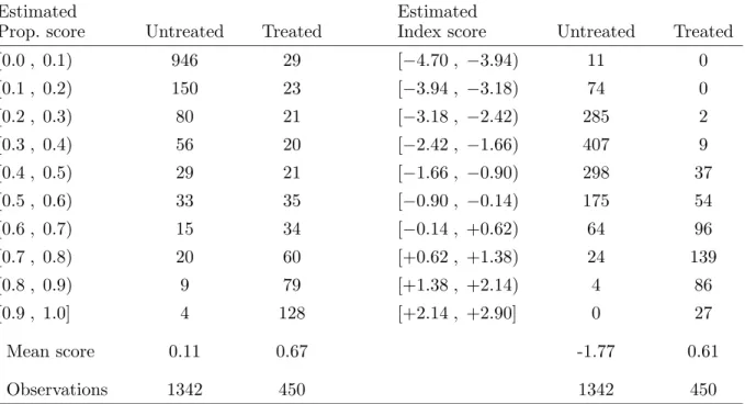
Table 2.1: Distribution of Estimated Propensity and Index Score.

Estimated Estimated

Prop. score Untreated Treated Index score Untreated Treated

[0.0, 0.1) 946 29 [−4.70, −3.94) 11 0

[0.1, 0.2) 150 23 [−3.94, −3.18) 74 0

[0.2, 0.3) 80 21 [−3.18, −2.42) 285 2

[0.3, 0.4) 56 20 [−2.42, −1.66) 407 9

[0.4, 0.5) 29 21 [−1.66, −0.90) 298 37

[0.5, 0.6) 33 35 [−0.90, −0.14) 175 54

[0.6, 0.7) 15 34 [−0.14, +0.62) 64 96

[0.7, 0.8) 20 60 [+0.62, +1.38) 24 139

[0.8, 0.9) 9 79 [+1.38, +2.14) 4 86

[0.9, 1.0] 4 128 [+2.14, +2.90] 0 27

Mean score 0.11 0.67 -1.77 0.61

Observations 1342 450 1342 450

Comparison of the number of treated and untreated individuals by propensity score and index score intervals.

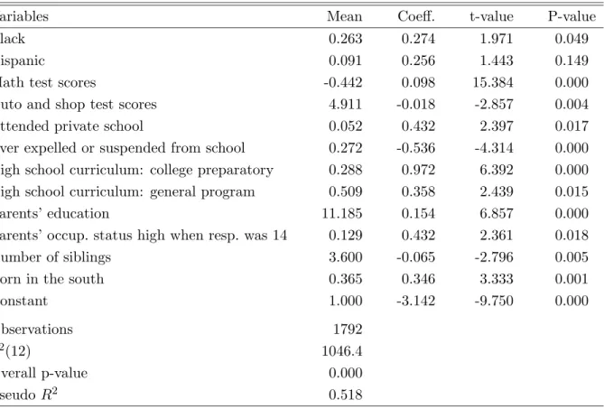
information about the high school career, and ability measures play an important role in modeling the selection decision to estimate the propensity score. The NLSY provides ten ability measures, the Armed Services Vocational Aptitude Battery scores. Since respon- dents participated in the tests at diﬀerent ages the scores are adjusted by regressing the raw scores on age dummies and using the residuals subsequently as explanatory variables, analogous to Blackburn & Neumark(1993). Math scores will be used to describe As

and parents’ education to describeF_s in equation (2.5).

The variables and the probit estimation are presented in appendix A. It successfully separates college and high school graduates which, unfortunately, makes matching at the boundaries a diﬃcult project. Note, however, that this aspect does not favor a linear model either because itsad hoclinear interpolations between the extremes would not necessarily be correct. Table 2.1 compares the absolute frequencies of treated and untreated men for certain propensity score and index score intervals. The index orprobitsis Φ⁻¹(ˆp),

real fundamental economic changes which is why $1000 would be removed. See e.g. the NLSY79 User’s Handbook (1997: p. 266): “... the calculation procedure [...] produces, at times, extremely low and extremely high pay rate values.”

(28)

where Φ is the cumulative normal density function. It is linear in the matching vari- ablesX and might be better suited to reﬂect the underlying distribution of the estimated propensity scores.

Using ˆpmight make individuals at the high end of the propensity score scale look more similar than they actually are and, analogously, make individuals at the low end look more identical. Indeed, for low index scores, there are numerous untreated units in cells with hardly any treated while for low ˆpthere is still a reasonable number of treated units.

Matching on the index will drop countless low-score untreated individuals while matching on the propensity score will keep several of them. In the high end of the distribution, the situation is comparable but less pronounced. Results will be discussed for both matching on the propensity score and on the index. For the sake of brevity, “propensity score” will denote both scores in the main text below if closer speciﬁcation is not necessary.

Distance Measures

A propensity score caliper approach within cells deﬁned by race, age and high school graduation year is pursued, see e.g. Cochran & Rubin (1973). First, the cells are deﬁned. Only individuals of the same race are matched. Furthermore, the age structure is taken into account: individuals of the same age, one year younger or one year older are permitted to be matched. Similarly, only those who receive their high school degree in the same year, one year earlier or later than the treated may become potential controls.

This guarantees that untreated individuals within a stratum share a similar economic environment at the beginning of their treatment phase. Exact matches on age and the year of the high school diploma would be preferable, but would substantially reduce the number of potential controls.

Second, within these cells a pool of potential controls is generated for each treated by excluding all untreated units who exceed a certain propensity or index score caliper ε.

The ﬁnal decision of who becomes an actual control will then be made by minimizing either the Mahalanobis or the propensity score distance. The Mahalanobis distance is a weighted Euclidean distance d(x_t,x_c) = (x_t−x_c)V⁻¹(x_t−x_c), where x_t and x_c are the

(29)

vectors comprising the observable covariates of the treated and the potential control unit, respectively. V is the pooled covariance matrix of these variables which serves to norm the vectors. If the propensity score is inconsistently estimated the Mahalanobis metric within calipers might help circumvent possible problems. In sum, the distance is

d(x_t,x_c) =











∞ if |p(x_t)−p(x_c)|> ε (x_t−x_c)V⁻¹(x_t−x_c)

or |p(x_t)−p(x_c)| else.

(2.7)

An inﬁnite distance indicates that matching is forbidden.¹¹

Two diﬀerent caliper widths ε will be compared, a narrow and a broad one. For propensity score matching, the narrow one will be set equal to 0.05 while the broad one will be 0.10. For index score matching, the respective numbers are 0.30 and 0.60. They are chosen such that both matching on the propensity score and on the index employ an approximately equal number of treated units. Broad calipers allow matching more individuals at the expense of a potentially less favorable balance of covariates. Narrow calipers generate closer similarity of matched units but might have to drop several high- and low-score units. No calipers would have adverse consequences. First, any arbitrarily large distance between treated and controls would then be possible, and, second, matching algorithms would consume substantially more time.¹²

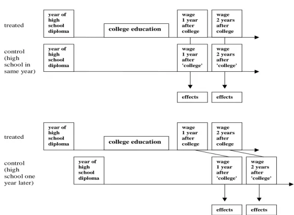
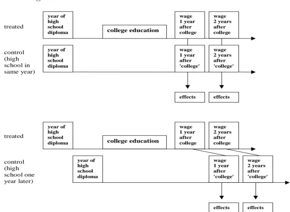
After having constructed the pool of potential controls appropriate wages serving as the counterfactual wages of the treated are assigned. The time span between the year in which the treated unit received his college degree and his high school diploma – the treatment phase – is added to the year in which his potential controls received their high school diploma. The result is considered as the counterfactual year in which his potential controls would have received a college degree. Note that the treatment phase is not necessarily just the years at college because the treated individual might have interrupted education for a while. Figure 2.1 illustrates the procedure. The counterfactual outcome

11Matching using the Mahalanobis distance is discussed in Rubin (1980). A comparison of three distance measures is provided inGu & Rosenbaum (1993). Furthermore, propensity score calipers are discussed inRosenbaum & Rubin (1985: 3)and Rosenbaum (1989: 3.4).

12In each step of the algorithm every treated would have to be compared to the whole control reservoir.

Given a caliper, the treated has to be compared to only a small number of suitable untreated units.

(30)

Figure 2.1: Illustration of the Evaluation Procedure.

treated

control (high school in same year)

treated

control (high school one year later)

wage 1 year after college

wage 2 years after college

wage 2 years after 'college' year of

high school

diploma college education

year of high school diploma

effects effects

year of high school

diploma college education

wage 1 year after college

wage 2 years after college

year of high school diploma

wage 1 year after 'college'

wage 2 years after 'college'

effects effects wage

1 year after 'college'

The ﬁrst diagram demonstrates the optimal case when treated and control individuals receive their high school diploma in the same year. The second indicates how things change when there is one year diﬀerence.

one year after treatment is the wage of the potential control one year after his hypothetical end of college. If wage information is missing the potential control is dropped for that year after treatment but is still used for other years. If the wage of the treated is missing the treated is removed, too. Ten years after college will be examined and each year will be stratiﬁed separately such that individuals who are removed in some year due to missing wage information may still be available in other years.

The Matching Algorithms

The ﬁnal decision regarding the matching procedure is how to implement the chosen matching criteria, in other words, how the distances between treated and controls is minimized. Three algorithms will be compared in this study, one greedy pair matching and two full matching, optimal full matching as proposed by Rosenbaum (1991) and an own greedy full matching. Greedy pair matching randomly selects one treated person