Near real-time observations of snow water equivalent for SIOS on Svalbard – (SWESOS)

(1)

Project report

Near real-time observations of snow water equivalent for SIOS on Svalbard – (SWESOS)

Authors:

Katharina Jentzsch (Alfred Wegener Institute for Polar and Marine Research, Potsdam) Niko Bornemann (Alfred Wegener Institute for Polar and Marine Research, Potsdam) William Cable (Alfred Wegener Institute for Polar and Marine Research, Potsdam) Jean-Charles Gallet (Norwegian Polar Institute)

Stephan Lange (Alfred Wegener Institute for Polar and Marine Research, Potsdam) Sebastian Westermann (University of Oslo)

Julia Boike (Alfred Wegener Institute for Polar and Marine Research, Potsdam)

Date:

September 24, 2020

(2)

iii

Abstract

Our project contributes to the SIOS observing system in the following ways: we evaluate a new automated monitoring technique for measuring snow water equivalent (SWE) using a passive gamma ray sensor at the Bayelva site (near Ny-Ålesund). Our goal is to provide high quality, continuous, near-real time data for the observation of SWE. The essential climate variables of snow cover (snow height, SWE, spatial coverage) and dynamics (timing of onset and melt, wetting) will be derived using the new automated sensor. We aim to provide a unique dataset by linking existing snow datasets with the new SWE measurements. This dataset will be essential to develop and calibrate snow, permafrost and hydrologic models in this data scarce region.

(3)

iv

1 Introduction

In the following section, we motivate our study by introducing its general scientific background and describe the research goals of our analyses.

1.1 General scientific background

The arctic environment is changing rapidly, as global warming causes ice, snow, and frozen ground—the components of the cryosphere—to melt and thaw. White snow, which strongly reflects sunlight, is being replaced by vegetation and bare soil, a darker surface, resulting in less energy being reflected back to space. This change causes further warming, leading to further melting, thawing and warming, thus contributing to the polar amplification. This positive feedback makes the reduction of the arctic snow cover a major influence on the climate system. Despite this importance, we know little about the local spatial variability and properties of arctic snow at scales below the current satellite resolution. Yet, it is this local scale, which is of interest for climatologists, biologists and modellers. For example, modelling subsurface temperature and stream runoff depends largely on local-scale snow-cover properties. Satellite records from the last five decades show that the spring snow is disappearing earlier, with greatest change (decline) in June (https://www.climate.gov/news- features/understanding-climate/climate-change-spring-snow-cover). The recent warming observed in Ny-Ålesund over the past 20 years amounts to about 1.46 ± 0.05 °C/decade (Bacher, 2019) which is due to the strong winter warming trend (Maturilli et al. 2015).

Seasonal snow is an important component of the Svalbard permafrost and hydrological system due to its water storage and insulation properties, but a lack of automated observations hampers understanding and forecasting for permafrost models or runoff in this region. The quantity of water contained within a snowpack, termed snow water equivalent (SWE), is one of the most important variables to consider, but difficult to accurately measure and model over broad spatial areas. Large discrepancies in SWE exist between estimates derived from different measurement techniques such as reanalysis products, precipitation gauges, and satellite observations. Many of the issues associated with SWE measurement and modelling are a result of the scarcity of reliable solid precipitation observations at high latitudes with which to calibrate and develop SWE products. Obtaining accurate in situ SWE observations is a difficult and time-consuming task. Automated methods of SWE measurement can increase the ease with which seasonal SWE patterns can be monitored and, unlike manual sampling techniques, do not invasively disturb a snowpack’s internal structure, allowing seasonal and long term monitoring. Continuous observations of snow properties in high-latitude such as Svalbard are (almost) non-existent and, consequently, calibrating the current generation of snow, permafrost and hydrologic models, is challenging. The development, calibration and improvement of more sophisticated SWE products in high latitudes call for a greater number of accurate precipitation observations with rigorously constrained uncertainties. Any new instrumentation must be validated against field data.

(5)

6

1.2 Specific aims of the project

We assess the accuracy, spatial representativeness and the applicability of the SWE and snow depth measurements using a new passive gamma ray sensor, together with automated snow depth measurements, time-lapse camera images and field observations at the Bayelva long term observational site close to Ny-Ålesund. In August 2019, we installed the new sensor, that measures snow water equivalent (SWE) automatically to quantify the evolution of SWE and snow depth over one winter (2019/2020) period. The goal is to assess the suitability of the monitoring system to provide reliable estimates of SWE and snow depth, which could be used to calibrate and develop SWE and snow models in this data-scarce region. We will make recommendations about how this setup could be extended into similarly remote environments to attain greater understanding of snow cover, its changes and variability in the future.

2 The Bayelva research site

The Bayelva site is located on western Spitsbergen about 3 km from the research base of Ny- Ålesund at 78°55’ N and 11°50’ Eand 25 m a.s.l. (Figure 2.1). The automatic weather, soil and permafrost station has collected data since 1998 and consists of sensors measuring snow depth, liquid precipitation, air temperature and humidity, wind speed and direction, and the incoming and outgoing components of shortwave and longwave solar radiation. Snow depth is measured automatically with three sensors as well as manually at fixed positions. Snow temperature is recorded at two heights and the snow dielectric constant (SDC) is measured hourly using a vertically installed Time Domain Reflectometry (TDR) probe inside the fence of the meteorological station (Figure 3.1). Since the TDR probe is 0.3 m long, reliable values of the SDC can only be recorded at snow depths exceeding 0.3 m. Time-lapse cameras provide an overview of the snow distribution within the fenced climate station, at the newly installed SWE site, as well as overlooking the larger area of the Bayelva catchment.

Figure 2.1: (a) Location of Ny-Ålesund on Svalbard (Norwegian Polar Institute n.d.). (b) Location of the study site in the Bayelva river catchment close to Ny-Ålesund. Thick black lines mark roads and contour lines give the height in meters above sea level (Lüers et al., 2014 as adapted from Westermann et al., 2009). (c) Topography surrounding the study site (Norwegian Polar Institute n.d.).

(6)

7

3 Measuring the snow water equivalent

This chapter deals with the snow water equivalent (SWE) measurements performed at the Bayelva site during the winter season 2019/2020. In section 3.1 the newly installed automated SWE system is presented. The manual measurements performed to validate the automatically recorded data will subsequently be described in section 3.2.

3.1 Automatic measurements

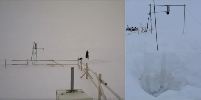
The SWE sensor is suspended from a horizontal pole at 2.42 m height above ground between two tripods and secured with guy wires. A SR50A (Campbell Scientific) snow depth sensor is installed next to the SWE sensor (Figure 3.1). Time-lapse cameras capture images of the surrounding area at least six times per day. The Campbell Scientific CS725 sensor calculates SWE passively measuring the attenuation of gamma rays emitted from naturally occurring isotopes of Potassium (⁴⁰K) and Thallium (²⁰⁸Tl) present in the substrate beneath the sensor.

No background data for the site’s emission of ⁴⁰K and ²⁰⁸Tl radiation levels were available prior to evaluate the application of this method. The SWE derived from the more abundant isotope is generally the more reliable (Smith C.D. et al., 2017). Since over the entire measurement period the instrument consistently detected more Potassium isotopes, our analysis is based on the SWE derived from the emission by ⁴⁰K. The CS725 calculates the SWE by integrating gamma ray emissions over a 24 h period before outputting an estimate of snowpack SWE at a 6 h time resolution. The instrument can measure the SWE of a snowpack up to ∼600 mm (about 1.5 m dry arctic snow) and has a measurement accuracy of ±15 mm from 0 to 300 mm and ±15 % from 300 to 600 mm. The CS725 covers an effective down looking field of view of

∼120°, allowing it to monitor the SWE of an area between ∼55 m² at zero snow depth and

∼25 m² at the maximum snow depth of about 0.8 m. The SWE measurement is most heavily weighted towards the snow directly beneath the sensor as gamma photon intensity is attenuated by greater travel distance through the snowpack with increasing radial distance.

The installed collimator reduces the surface area from which the gamma rays are sourced.

Depending on the snow depth, the SR50 monitors the snow depth over an area of between 1.3 m² and 0.6 m². Our site transmits data daily using a real-time connection to AWIPEV.

(7)

8 Figure 3.1: Instrument setup of the Bayelva SWE station including a schematic visualization of the footprint areas of the automated snow depth and SWE sensor.

3.2 Manual measurements

We had originally planned manual sampling about once per month between November and February and at least once per month after March; however, we only managed to sample in November and then again in March, April and May. This was (a) due to lack of snow in November rendering access very difficult; (b) for safety reasons, as it is not allowed to walk so far from Ny-Ålesund during polar night conditions (polar bear safety); and (c) due to the start of the COVID pandemic in spring which resulted in a general shortage of personnel at the station and for the ARCSNOW project.

The manual measurements consist of measuring the snow depth and weighing a known volume 𝑉𝑠 of snow to within ± 0.01 kg using a steel tube with a radius 𝑅 of 0.04 m and a length of 0.6 m following the procedure in figure 3.2. If the snow depth exceeds 0.6 m the measurement has to be performed in more than one layer, which can add some uncertainty to the recorded values. In each measurement session, several snow pits were dug in a radial pattern around the automatic SWE system, covering approximately the same area as covered by the footprint of the CS725 in order to validate the automatic measurements and capture some of the snow variability.

(8)

9 Figure 3.2: Procedure to measure the snow depth and weight of a snow column using a steel tube.

The snow density 𝜌_𝑠 is calculated from the measurements of snow depth ℎ and mass 𝑚_𝑠 via

𝜌_𝑠[ 𝑔

𝑐𝑚³] = 𝑚_𝑠[𝑔]

𝑉𝑠[𝑐𝑚³]= 𝑚_𝑠[𝑔]

𝜋𝑅[𝑐𝑚]²ℎ[𝑐𝑚]= 𝑚_𝑠[𝑔]

50𝑐𝑚²ℎ[𝑐𝑚].

Considering that the mass of the snow column inside the cylinder 𝑚_𝑠 is equal to the mass of the water 𝑚_𝑤 resulting from melting this snow volume, the SWE can be calculated from the density of snow, using a water density 𝜌_𝑤 of 1 gcm^-3 and the snow depth:

𝑚𝑠= 𝑚𝑤

𝜌_𝑠∙ 𝑉_𝑠 = 𝜌_𝑤∙ 𝑉_𝑤 𝜌_𝑠𝜋𝑅²ℎ = 𝜌_𝑤𝜋𝑅²𝑆𝑊𝐸

(9)

10 𝑆𝑊𝐸 =𝜌_𝑠ℎ

𝜌_𝑤.

Inserting the expression for the snow density from above gives

𝑆𝑊𝐸 = ℎ𝑚_𝑠

𝜌_𝑤50𝑐𝑚²ℎ= 𝑚_𝑠 𝜌_𝑤50𝑐𝑚².

Inserting the density of water and transforming into units of mm results in

𝑆𝑊𝐸[𝑚𝑚] = 𝑚_𝑠[𝑔]

𝜌𝑤[𝑔/𝑐𝑚³]50𝑐𝑚²∙ 10𝑚𝑚

𝑐𝑚 = 𝑚_𝑠[𝑔]

1𝑔/𝑐𝑚³∙ 50𝑐𝑚²∙ 10𝑚𝑚 𝑐𝑚

=𝑚_𝑠[𝑔]

50 𝑔 𝑐𝑚

∙ 10𝑚𝑚

𝑐𝑚 = 0.2𝑚𝑚

𝑔 ∙ 𝑚_𝑠[𝑔].

4 Evolution of SWE and snow depth over the measurement period

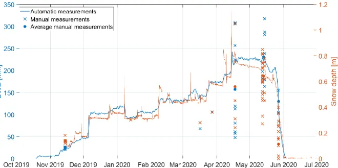
Figure 4.1 shows the evolution of SWE and snow depth over the 2019/2020 snow season at the Bayelva site. Automated SWE measurements are available since 18.10.2019, while the time series of valid snow depth records starts on 15.11.2019. The courses of snow depth and SWE are very similar. Both variables increase until reaching a maximum in the middle of April 2020 of about 0.8 m and 225 mm respectively. Afterwards the SWE remains almost constant until mid-May 2020 while the snow depth begins to slightly decrease. At the end of May 2020 finally a strong decline in both snow depth and SWE sets in. By the beginning of June 2020 the area is snow free and both variables return to zero.

While in November 2019 the individual manual measurements within the footprint area of the SWE sensor are close together, they show a larger spread around the curves of automatic measurements in spring 2020. Due to this large spatial variation, the annual cycle of snow depth and SWE is not visible from the manual measurements.

Figure 4.1: The evolution of the automated six hourly SWE and hourly snow depth records over the winter period 2019/2020 compared to the sporadic manual snow pit measurements.

(10)

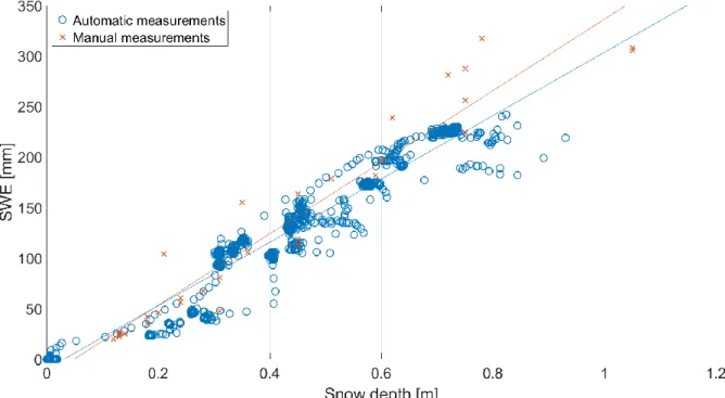
11 Figure 4.2 reveals the expected strong positive linear correlation between snow depth and SWE for both manual and automatic measurements.

Figure 4.2: Relationship between SWE and snow depth during the measurement period based on manual and automated measurements. The lines represent the respective least squares linear regression.

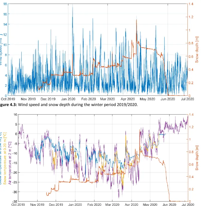
Further measurements performed within the fenced area of the Bayelva climate station help to explain the observed variations in snow depth and SWE. For example peaks or strong and abrupt in- or decreases in snow depth and SWE which occur at times of high wind speeds indicate a transport of snow by the wind (Figure 4.3). The intensity of this wind drift furthermore depends on the temperature and the water content of the snow cover. Dry and soft, i.e. cold snow, as was present most of the winter (November to April) is most prone to wind drift (Figure 4.4). The fence surrounding the climate station furthermore promotes the formation of snow dunes. Next to verifying the onset and end of the snow-covered season, the surface albedo can indicate periods of strong snow-fall (Figure 4.5). For example, the high albedo of fresh snow indicates that the increase in snow depth and SWE at the end of May 2019, just before snow-melt, is related to a snow-fall event.

(11)

12 Figure 4.3: Wind speed and snow depth during the winter period 2019/2020.

Figure 4.4: Snow temperatures at 0.04 and 0.20 m above the ground, 2 m air temperature and snow depth during the winter period 2019/2020.

(12)

13 Figure 4.5: Surface albedo and snow depth during the winter period 2019/2020.

5 Snow density

Similar to the snow depth, the snow density is highly variable over time. In order to capture its evolution over the course of a winter season, regular and thus automated measurements are needed. Hence, in the following, we evaluate the suitability of the automatic SWE system to provide reliable estimates of the snow pack bulk density. Therefore, we combine the automatically measured snow pack SWE and snow depth estimates to calculate the snow density. Additionally, we derive the snow density from nearby automated measurements of the SDC and compare both calculated time series with the manual snow pit measurements.

5.1 Theory

In the following subsections, we will derive the equations used to calculate the snow density from the manual snow pit measurements, the automated SWE and snow depth measurements and the automated SDC records.

5.1.1 Manual measurements

As already described in section 3.2 the snow density 𝜌_𝑠 can be calculated from the manual measurements using

𝜌_𝑠[ 𝑔

𝑐𝑚³] = 𝑚_𝑠[𝑔]

𝑉_𝑠[𝑐𝑚³]= 𝑚_𝑠[𝑔]

𝜋𝑅[𝑐𝑚]²ℎ[𝑐𝑚]= 𝑚_𝑠[𝑔]

50𝑐𝑚²ℎ[𝑐𝑚]. 5.1.2 Automated SWE and snow depth measurements

The mass of the snow cover 𝑚_𝑠 above a unit area of 1 m² has to equal the mass of the water 𝑚_𝑤 resulting from melting this snow cover:

𝑚_𝑠 𝑚² = 𝑚_𝑤

𝑚²

𝜌_𝑠 ∙ 𝑉_𝑠

𝑚² = 𝜌_𝑤∙ 𝑉_𝑤 𝑚²

𝜌_𝑠𝑚²

𝑚²ℎ = 𝜌_𝑤𝑚² 𝑚²𝑆𝑊𝐸

(13)

14 𝜌_𝑠ℎ = 𝜌_𝑤𝑆𝑊𝐸.

Thus, the snow density 𝜌_𝑠 can be calculated from the SWE using the density of pure water at 0 °C 𝜌_𝑤 of 0.99987 gcm^-3 and the snow depth ℎ via

𝜌_𝑠[ 𝑔

𝑐𝑚³] =𝜌_𝑤[ 𝑔

𝑐𝑚³] 𝑆𝑊𝐸[𝑐𝑚]

ℎ[𝑐𝑚] . 5.1.3 Automated SDC measurements

According to Roth et al. (1990), the volumetric liquid water content 𝜃_𝑤 of a snow cover can be estimated from snow dielectric measurements, using

𝜃_𝑤= 𝑑_𝑠^𝜔−(1 − 𝜂)∙ 𝑑_𝑖^𝜔− 𝜂 ∙ 𝑑_𝑎^𝜔 𝑑_𝑤^𝜔− 𝑑_𝑎^𝜔 ^,

where 𝑑_𝑠 denotes the snow dielectric constant (SDC), as obtained from automatic half-hourly Time Domain Reflectometry (TDR) measurements at the Bayelva site and 𝑑_{𝑎,𝑤,𝑖} stand for the dielectric constants of air, water and ice, respectively, as documented in the literature (Table 5.1).

The porosity of the snow cover 𝜂 is given by

𝜂 =𝜌_𝑠 − 𝜌_𝑖− 𝜃_𝑤(𝜌_𝑎− 𝜌_𝑤) 𝜌_𝑎− 𝜌_𝑖 ^.

Assuming a dry snow cover, that means 𝜃_𝑤 = 0, combining the latter two equations and inserting values for the density of air, ice and water 𝜌_{𝑎,𝑖,𝑤} from the literature (Table 5.1) allows to additionally estimate the snow density from the snow dielectric constant:

𝜌_𝑠= (𝜌_𝑎− 𝜌_𝑖)𝑑_𝑠^𝜔− 𝑑_𝑖^𝜔 𝑑_𝑖^𝜔− 𝑑_𝑎^𝜔+𝜌_𝑖, assuming 𝜔=0.5 (Roth et al. 1990).

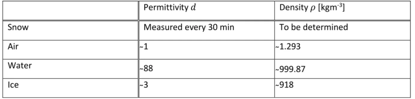
Table 5.1: Approximate permittivity and density values of snow, air, water and ice at 0 °C and at an atmospheric pressure of 1013.25 hPa. Snow permittivity is obtained from automated measurements every 30 minutes while the remaining values are taken from the literature. The temperature and pressure dependency of the densities are ignored in this context.

Permittivity 𝑑 Density 𝜌 [kgm^-3]

Snow Measured every 30 min To be determined

Air ̴1 ̴1.293

Water ̴88 ̴999.87

Ice ̴3 ̴918

(14)

15

5.2 Comparison

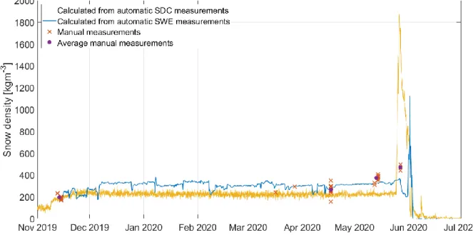
Figure 5.1 shows the course of the snow density over the measurement period as obtained from manual measurements as well as calculated from the automatic SWE and SDC records.

Between the end of November and the beginning of December 2019 the snow density time series agree very well. While the density calculated from the SDC stays constant and most likely too low, with values slightly over 200 kgm^-3 until May 2020, the density based on the SWE rises to slightly higher values of about 300 kgm^-3. Furthermore, the latter time series shows more variation, related to the natural variability of the snow cover, which is further intensified by the often windy conditions on Svalbard. The manual measurements during this period correspond equally well to both time series. Only the manual measurements on May 12 and 14, 2020 yield values agreeing better with the ones calculated from the SWE. The snow density based on the SDC rises to unrealistic values when the snowmelt sets in in the second half of May 2020. This is probably related to the assumption of dry snow, which is not met anymore. The snow density derived from the SWE measurements takes on unrealistically high values for a shorter period at the end of the snow melt starting at the beginning of June 2020.

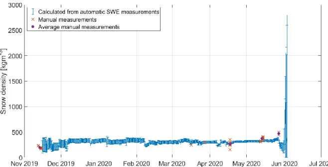
Figure 5.2 reveals that this is related to the insufficient precision of the SWE and snow depth measurements at very low measurement values below 0.1 m for snow depth and a SWE lower than 25 mm. The uncertainty range indicated by the error bars is calculated based on the rules of error propagation from the uncertainty of the SWE and snow depth measurements as

∆𝜌_𝑠 = 𝜕𝜌_𝑠

𝜕𝑆𝑊𝐸+𝜕𝜌_𝑠

𝜕ℎ =𝜌_𝑤

ℎ ∆𝑆𝑊𝐸 −𝜌_𝑤 ∙ 𝑆𝑊𝐸 ℎ² ∆ℎ.

Compared to the SDC measurements the automatic SWE records can be used to reliably assess the snow density longer into the snowmelt period. Furthermore, as opposed to the SWE, the snow dielectric constant is distorted when the snow depth is below the length of the vertically installed TDR probe of 0.3 m.

Figure 5.1: Course of the snow density as obtained from manual measurements as well as calculated from the automatic SWE and SDC measurements over the winter season 2019/2020.

(15)

16 Figure 5.2: Course of the snow density as obtained from manual measurements as well as calculated from the automatic SWE measurements over the winter season 2019/2020. The error bars indicate the uncertainty range of the calculated snow density.

We therefore manually removed the unrealistically high density values associated with sensor insufficiencies during the snow melt period (Figure 5.3).

Figure 5.3: Course of the snow density as obtained from manual measurements as well as calculated from the automatic SWE and SDC measurements over the winter season 2019/2020 after removing the unrealistically high values during the snow melt period from the automated time series.

(16)

17

6 Spatial variability of SWE, snow depth and snow density

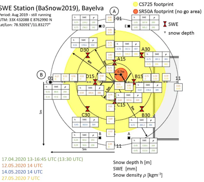
Figure 6.1 provides an overview of the spatial distribution of all manual snow pit measurements during the winter period 2019/2020 within the footprint area of the automated SWE sensor.

Figure 6.1: Overview of all snow depth, SWE and snow density records derived from manual snow balance tube measurements within the footprint area of the automated SWE sensor.

Figures 6.3, 6.5 and 6.7 compare the manual measurements of snow depth, SWE and snow density inside the footprint area of the automated SWE sensor to the respective variables derived from the automated measurements for the three individual sessions of manual measurements in April and May 2020. Table 6.1 provides an overview of the range of manual measurements and their average values compared to the corresponding automated records.

As already visible in figure 4.1, the manual measurements show a high spatial variability.

On 17.04.2020, the continuous snow cover can be subdivided into two distinct layers (Figure 6.2). At the bottom, there is a dirty snow layer which indicates the advection of dust from various local sources, which were exposed due to the exceptionally thin snow cover during the measurement period. At the top, there is an ice layer, which is caused by the temperatures above 0 °C during an early warm event, persisting for several days in mid-April (see Figure 4.4).

(17)

18 Since there was very little snow fall during the measurement period, the site is clearly strongly affected by windblown snow.

Figure 6.2: Continuous snow cover on 17.04.2020.

(18)

19 Figure 6.3: Spatial distribution of the manual snow depth, SWE and snow density measurements as well as the automatic measurements standing for the larger footprint area of the automated sensors (Figure 5.1) on 17.04.2020.

(19)

20 Figure 6.4: Continuous snow cover on 12.05.2020 (upper image) and 14.05.2020 (lower image).

(20)

21 Figure 6.5: Spatial distribution of the manual snow depth, SWE and snow density measurements as well as the automatic measurements standing for the larger footprint area of the automated sensors (Figure 5.1) on 12. and 14.05.2020.

(21)

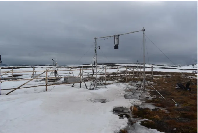
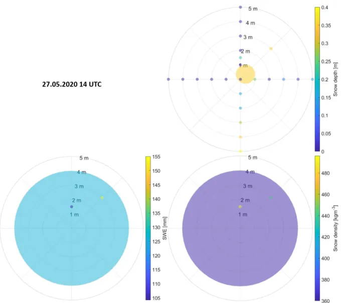
22 Figure 6.6 reveals a discontinuous snow cover on 27.05.2020 characterized by alternating patches of snow free and snow covered ground.

Figure 6.6: Discontinuous snow cover on 27.05.2020.

(22)

23 Figure 6.7: Spatial distribution of the manual snow depth, SWE and snow density measurements as well as the automatic measurements standing for the larger footprint area of the automated sensors (Figure 5.1) on 27.05.2020.

Table 6.1: Minimum, maximum, average values and value range of the snow depth, SWE and snow density for the three sessions of manual measurements as well as the corresponding values obtained from the automated sensors.

17.04.2020 12./14.05.2020 27.05.2020

h [m] SWE [mm] 𝜌_𝑠 [kgm^-3] h SWE 𝜌_𝑠 h SWE 𝜌_𝑠

Min 0.24 48 154 0.27 164 308 0 104 442

Max 1.05 308 342 0.85 317 407 0.40 155 496

Range 0.81 260 188 0.58 154 99 0.40 51 54

Mean 0.56 157 264 0.64 231 365 0.11 130 469

Auto 0.82 218 270 0.69 226 324 0.35 126 360

With only one exception, all automatic measurements lie within the range of the manual measurements. However, the range of up to 260 mm between simultaneous manual SWE measurements at different locations within the footprint area exceeds the annual variation of the SWE of about 225 mm. Therefore, it is questionable if the spatial resolution of the automated SWE sensor is sufficient to capture the extremely high spatial variability of the SWE

(23)

24 inside the already relatively small footprint area. Likewise, with a spatial variation of up to 0.81 m within the footprint area of the SWE sensor, the spatial variability of the snow depth equals its temporal variation over the snow-covered period. Therefore, the smaller footprint of the snow depth sensor might not be representative of the whole footprint area of the SWE sensor, leading to considerable uncertainties when combining both measurements to calculate the snow density. In the three examples, the spatial variation of snow depth and SWE increases with their absolute values. However, it has to be taken into account that the number of individual manual measurements differs significantly between the three measurement sessions.

7 Conclusions

We could verify the onset and end of the snow-covered season as well as strong changes in snow depth and SWE as indicated by the new automated sensors using independent wind, temperature and radiation data from the nearby climate station. The new automated measurement system thus reliably captures the general evolution of these snow properties over the snow-covered season.

A major problem of the automated SWE measurements is the high spatial variability of SWE and snow depth within the footprint area of the sensor due to an uneven snow cover associated with an uneven terrain, wind drift and a discontinuous snow cover due to patchy snow melt. Hence, the automated measurements are expected to best represent the snow conditions inside their footprint area at sites with an even snow cover associated with a flat surface, no large obstacles and low wind speeds. More manual measurements would have been useful to better evaluate the course of the spatial variability over the winter season.

Acknowledgement

We thank the AWIPEV station for their continuous support in maintaining the Bayelva site and measuring snow characteristics. This work was supported by the Research Council of Norway, project number 291644, Svalbard Integrated Arctic Earth Observing System – Knowledge Centre, operational phase.

References

Bacher, S. M., 2019. Enhanced Warming and Wetting of the Active Layer Caused by Rain and Snow, Svalbard.

Bachelor thesis (unpublished), University of Potsdam, Potsdam, Germany.

Ebenhoch, S., 2018. Discussion of the thermo-insulation effect of a seasonal snow cover on permafrost soil in Bayelva, Svalbard (1998 - 2017) with respect to current knowledge. Master thesis (unpublished), Heidelberg University, Heidelberg, Germany.

Lüers, J., Westermann, S., Piel, K., Boike, J., 2014. Annual CO2 budget and seasonal CO2 exchange signals at a High Arctic permafrost site on Spitsbergen, Svalbard archipelago. Biogeosciences 11 (1). 10.5194/bgd-11-1535- 2014.

Maturilli, M., Herber, A., König-Langlo, G., 2015. Surface radiation climatology for Ny-Ålesund, Svalbard (78.9°

N), basic observations for trend detection. Theor. Appl. Climatol. 120, 331–339. 10.1007/s00704-014-1173- 4.

Norwegian Polar Institute, n.d., Maps of Svalbard, Retrieved from https://toposvalbard.npolar.no on 2020-04- 08.

(24)

25 Smith, C., Kontu, A., Laffin, R., Pomeroy, J. W., 2017. An assessment of two automated snow water equivalent instruments during the WMO Solid Precipitation Intercomparison Experiment. The Cryosphere 11, 101-116.

10.5194/tc-11-101-2017.

Westermann, S., Lüers, J., Langer, M., Piel, K., Boike, J., 2009. The annual surface energy budget of a high-arctic permafrost site on Svalbard, Norway. The Cryosphere 3 (2), 245–263. 10.5194/tcd-3-631-2009.