https://doi.org/10.1007/s12080-020-00453-y ORIGINAL PAPER
Harvesting a remote renewable resource
Thorsten Upmann1,2,3 ·Stefan Behringer4
Received: 14 June 2019 / Accepted: 20 February 2020
©The Author(s) 2020
Abstract
In standard models of spatial harvesting, a resource is distributed over a continuous domain with an agent who may harvest everywhere all the time. For some cases though (e.g., fruits, mushrooms, algae), it is more realistic to assume that the resource is located at a fixed point within that domain so that an agent has to travel in order to be able to harvest. This creates a combined travelling–and–harvesting problem where slower travel implies a lower travelling cost and, due to a later arrival, a higher abundance of the resource at the beginning of the harvesting period; this, though, has to be traded off against less time left for harvesting, given a fixed planning horizon. Possible bounds on the controls render the problem even more intricate. We scrutinise this bioeconomic setting using a two-stage optimal control approach, and find that the agent economises on the travelling cost and thus avoids to arrive at the location of the resource too early. More specifically, the agent adjusts the travelling time so as to be able to harvest with maximum intensity at the beginning and the end of the harvesting period, but may also find it optimal to harvest at a sustainable level, where the harvesting and the growth rate of the stock coincide, in an intermediate time interval.
Keywords Optimal travelling–and–harvesting decision·Spatial renewable resource·Bioeconomic model·Two-stage optimal control problem·Sustainable harvesting
Introduction
The spatial dimension has recently attracted substantial attention in the economic literature on management of renewable resources. Frequently, this literature focuses on how much effort is required to harvest a resource when that resource is moving (e.g., fish or game).1 In this paper, we
1See, for example, Neubert (2003), Neubert and Herrera (2008), Brock and Xepapadeas (2008), Brock and Xepapadeas (2010), Ding and Lenhart (2009), Moeller and Neubert (2013), Kelly et al. (2016), and Grass et al. (2019).
Thorsten Upmann
Thorsten.Upmann@hifmb.de Stefan Behringer
Stefan.Behringer@sciencespo.fr
1 Helmholtz-Institute for Functional Marine Biodiversity at the University of Oldenburg (HIFMB), Ammerl¨ander Heerstraße 231, 23129 Oldenburg, Germany
2 Bielefeld University, Bielefeld, Germany
3 CESifo, Munich, Germany
4 Sciences Po, Department of Economics, 28 rue des Saints P`eres, 75007 Paris, France
reverse this premise: we consider the case where an agent is required to move in order to harvest an immobile resource.
Since travelling is a pre-requisite of harvesting, this implies a spatio-temporal interdependence of both policies, which is the focus of this paper.
The management of renewable natural resources has been a central issue in economics for many decades, and meanwhile the early models have been extended and generalised in various respects.2 While the temporal dimension of bioeconomic problems has been considered already in the early works, the spatial dimension became of interest to economists rather late, although it had been treated in the theoretical biology and applied mathematics literature for some time. Only in 1999, Sanchirico and Wilen generalise the fundamental open-access models of Gordon (1954) and Smith (1968). They set up a bioeconomic model with a finite number of resource patches within which the resource migrates, resulting in time-dependent changes in
2For example, Fan and Wang (1998) generalise the optimal harvesting policy of an autonomous harvesting problem with logistic growth to a non-autonomous case with periodic coefficients; Liski et al. (2001), accounting for costly changes of the harvesting rate, explore the effects of increasing returns to scale for a standard fishery management model; and Feichtinger et al. (2003), Hritonenko and Yatsenko (2006), Tahvonen (2008,2009a,b), Skonhoft et al. (2012), Tahvonen et al.
(2013) and Belyakov and Veliov (2014) investigate harvesting of age-structured populations.
the allocation of harvesting effort between these patches.
In this way, Sanchirico and Wilen (1999) integrate within- and between-patch biological and economic forces and demonstrate how these effects determine the process of bioeconomic convergence over space and time.
Following Sanchirico and Wilen (1999), the early models in spatial resource economics feature discrete patches, where migration of the biomass is modelled as entry and exit of the biomass from one location to the other. An alternative approach assumes a continuous distribution of the resource and models the migration and the spread of the biomass as diffusion; notable contributions are, for example, Montero (2000, 2001), Neubert (2003), Brock and Xepapadeas (2008, 2010), Ding and Lenhart (2009), Grass et al. (2019). An overview of the literature of spatial- dynamic systems in resource economics is provided by Conrad and Smith (2012) and Kroetz and Sanchirico (2015), for example.
In both strands of the literature, it is the resource that is mobile, while a possible movement of the agent remains unrecognised. In many instances, an immobile agent represents a reasonable simplification, as the effect of the agent’s movement can be neglected without losing much realism (e.g., coastal fixed–net fishery or shooting game)—but in other cases it is not. For example, in fruit and mushroom harvesting (in distant, vast wilderness such as Canada or Kamchatka), in forestry and in extensive agriculture, it is the agent who is moving to a resource that is positioned at a fixed location. In these cases, the travelling costs are often significant due to either large distances or because of a lack of infrastructure. Moreover, there is frequently only a fixed time slot in which the resource can be harvested, imposing constraints on the arrival time; for example, grape harvesting needs to be done within the last few days before the first night frost (late harvest). Another example, which has recently attracted much attention and for which travelling is essential, is algae:
a rapidly growing renewable resource, which may be used in the production of human and animal food, cosmetics, pharmaceuticals, chemicals, plastics, and biofuel.3Algae is frequently located at distant patches and is hard to monitor;
in particular, algae farms have now often been automated and located more and more off-shore so that travelling times become increasingly relevant.
Few papers consider a travelling–and–harvesting prob- lem of an agent in a spatial domain. Notable examples are Robinson et al. (2008), Behringer and Upmann (2014), Sir´en and Parvinen (2015), Belyakov et al. (2015,2017) and Zelikin et al. (2017), who consider an immobile resource
3For the possibilities of algal biofuel production, see, for example, Shurin et al. (2013), Zhu et al. (2017), Ummalyma et al. (2017), and Chu (2017); for a paper investigating algae growth control from a pollution point of view, see Yoshioka and Yaegashi (2018).
positioned at known locations. Except for Robinson et al.
(2008) and Sir´en and Parvinen (2015), these authors analyse a resource that is continuously distributed on the periphery of a circle and an agent who leaves for a round trip, return- ing home after each turn. In those models, the agent does not need to stop in order to harvest the resource, but is able to do thisen passant. While in the model of Behringer and Upmann (2014) the harvesting activity does not cost any time over and above the time of travelling, in Belyakov et al.
(2015, 2017) the maximal harvesting activity is inversely proportional to velocity. Models of the latter type are some- times referred to assearch models, because a higher speed of travelling renders the agent incapable of descrying much of the resource (see also Robinson et al.2002). However, in both types of models, i.e., in Behringer and Upmann (2014) and in Belyakov et al. (2015,2017), the travelling and the harvesting activity occur simultaneously.
Complementary to that approach are sequential travelling–and–harvesting decisions, which have previously been considered by Robinson et al. (2008) and Sir´en and Parvinen (2015), for example. In Robinson et al. (2008), the resource is located at discrete patches, and the agent is required to travel to those locations in order to be able to harvest. Sir´en and Parvinen (2015) modify that model and formulate a continuous–time, continuous–space version.
In those models, travelling and harvesting are mutually exclusive activities, taking place at different locations at subsequent times. Yet, in both models the decisions about travelling and harvesting are connected via a gathering- specific cost function. This formalises the idea that the travelling time, and hence the travelling cost, increases in the total amount already harvested, assuming that the harvest has to be carried back to a local market.
In Sir´en and Parvinen (2015), speed is assumed to be fixed (thereby invalidating their peculiar assumption that travelling costs are decreasing in speed). As a consequence, travelling costs are linearly increasing in the travelling distance, so that it is the distance, rather than the speed, on which the agent has to decide. In this way, travelling and harvesting decisions collapse, similar to search models.
Sir´en and Parvinen (2015), considering a infinite time horizon, show that in the steady state, the stock is an increasing function of the distance, while also the harvest increases with distance, before it eventually drops to zero.
In these spatio-temporal harvesting models, travelling to the resource constitutes a crucial activity. In particular, in their numerical analysis Robinson et al. (2008) show that the travelling costs dissipate a substantial fraction of the harvesting yield, and thus of the resource value. Because of this significance of the travelling cost, they obtain cyclical solutions with extraction varying over space and time, where the number of periods is sensitive with respect to parameterisation of the model.
The prediction of cyclical solutions with extraction varying over space and time, developed by Robinson et al.
(2008), resemble those in the continuous time model of Belyakov et al. (2015). These authors, specifying a long- run average objective to motivate a sustainability goal, show the existence of an optimal solution that also reveals a periodic structure with possibly exhausted areas appearing on the periphery of a circle. However, the presence of cyclical solutions is critically dependent on the assumption of harvesting capacity being inversely related to speed, as it is assumed in search models. Behringer and Upmann (2014) and Zelikin et al. (2017) relax this assumption and allow for two fully independent controls for speed and harvesting. Disentangling speed and harvesting, the latter authors obtain non-cyclic, and in some special cases even constant solutions.
In this paper, we also “disentangle” speed and harvesting, but with respect to the time dimension. We consider a two- stage optimal control problem with travelling and harvesting taking place in subsequent periods. In this way, travelling and harvesting are independent in the sense that they are only connected by the arrival time of the agent at the location of the resource. At the same time, travelling and harvesting are mutually exclusive, rival activities: the more time is spent on travelling, the less time is left for harvesting, and vice versa. The link by the arrival time yields a truly dynamic two-stage optimal control problem with two interconnected sub-problems: a travelling problem and a subsequent harvesting problem.
Our model shares some similarities with the timber gathering model of Robinson et al. (2008) and, in particular, with the continuous–time, continuous–space model of Sir´en and Parvinen (2015). In all three models, travelling and harvesting take place at different locations at subsequent times. However, in our model there neither is a functional link between the cost of travelling and the cost of harvesting, nor is there the need to carry the harvest back to some home market, but the resource is immediately sold at a market (or to a distributor) that is located close to the resource. (For a model that investigates the effects of endogenous market demands in a spatial harvesting setting see Anit¸a et al. 2019.) In the absence of such nearby markets, Robinson et al. (2008) allow for low levels of resource density to appear far from the harvester’s home with abundant resources in between, generalising the monotone predictions of Sir´en and Parvinen (2015).
Similarly, Belyakov et al. (2015), assuming an infinite time horizon, allow for a periodic structure with possibly exhausted areas. In our model, though, we investigate the behaviour of an agent with a finite rather than an infinite planning horizon. This perspective necessarily constrains
the time the agent may employ for harvesting once the resource is reached, rendering the eventual resource pattern a function of temporal and transport constraints.
To specify our two-stage travelling–and–harvesting control problem, we assume a linear–quadratic travelling cost, and consider two different possible specifications for the growth process of the resource: exponential growth and logistic growth. Applying these specifications, we analytically derive the optimal travelling–and–harvesting policies, i.e., the optimal paths, and the associated profits for both types of growth functions, thereby demonstrating the interdependence between both problems. The need for travelling requires the agent to weigh the benefit of an early arrival, i.e., a longer harvesting period, with its cost: a higher pecuniary travelling cost and a shorter time for the resource to grow, implying a lower stock upon arrival and hence less beneficial conditions for harvesting. In essence, the limited amount of time (fixed time period) encourages the agent to start harvesting early, while the presence of travelling costs lets the agent postpone the beginning of the harvesting period.
More specifically, we show that the optimal policies for exponential and logistic growth feature similar characteris- tics depending on two fundamental parameters: the planning horizon and the harvesting capacity (maximal effort level).
Given those parameters, the travelling period provides the agent with the possibility to customise the length of the harvesting period by choosing the arrival time. Since early arrival is costly in terms of higher travelling cost, the agent adjusts the speed of travelling to avoid being idle. As a con- sequence, optimal harvesting is done either at the maximal rate all the time, or harvesting is reduced to a sustainable level during an intermediate time interval. The latter policy with two switches in the harvesting intensity (maximum—
sustainable—maximum) only occurs in case of the logistic growth function. Finally, we also investigate the sensitiv- ity of our results with respect to the presence of bounds on the control of movement and with repect to the rate at which future revenues and costs are discounted. We show that, even though these modifications lead to some shifts in the optimal policy, the basic effects still prevail.
The rest of the paper is structured as follows: In Section
“The model” we set up the model. In Section “Decomposition of the problem” we decompose the travelling–and–harvesting problem into the two sub-problems. We begin our analysis with the harvesting problem in Section “Second stage:
harvesting”, and we then proceed with an analysis of the full travelling–and–harvesting problem in Section “First stage: optimal travelling–and–harvesting policy”. In Section
“Robustness of the results” we discuss the robustness of our results with respect to bounds on the control and the
discount rate, before we conclude in Section “Conclusion”.
The robustness analysis is relegated to AppendixA; longer proofs, to AppendixB.
The model
We consider an economic agent who has the exclusive right to harvest a renewable natural resource during a fixed, finite time period T ≡ [0, T]. We may think of a harvesting licence or a rental period that begins at timet = 0 and terminates at t = T.4 The resource is situated at some fixed and known locationx1 ∈ (0,x¯]. At timet ∈ T the location of the economic agent isx(t)∈X ≡ [0,x¯], with the agent’s initial location given byx(0)=0. The agent is able to harvest the resource only at his/her current position, and sincex(0) = x1, the agent is required to travel to get access to the resource. Only on arrival at locationx1is the agent able to begin with harvesting. The agent’s problem is thus a combined travelling–and–harvesting problem, where the speed of travelling, and hence the arrival time, and the harvesting rate have to be determined jointly in order to maximise the total profit, composed of the revenue from harvesting net of harvesting and travelling costs.
In order to move from one location to the next, the agent has to adjust the velocity of travelling v(t) ∈ V ⊂ R. This speed of movement (or the harvesting machine) cannot be chosen directly, though, but is physically controlled by means of accelerationa(t)∈ A ⊂ R. Thus, movement is described by
˙
x(t)=v(t), v(t)˙ =a(t), ∀t ∈T withx(0)=v(0)=0.
(1a) Specifying acceleration, rather than speed, as the control variable avoids the occurrence of unrealistic, i.e., discontin- uous speed profiles where the agent may abruptly switch speeds. (This specification of the movement model follows Pontryagin et al.1962; L´eonard and Long1992, Sec. 8.1;
Hull2003, Sec. 17.7 and others; a more sophisticated model can be found in, e.g., Bertolazzi and Frego 2018.) There may be lower and upper bounds on acceleration. For the moment, we disregard such constraints, but we shall assume in AppendixA, that acceleration is bounded bya(t)∈A ≡ [a
¯,a¯]witha
¯ <0 anda >¯ 0.5
4With an infinite time horizon the significance of the travelling period will reduce and the trade-off between the travelling and the harvesting decision will be less pronounced; also, any end–of–period effects will vanish.—All of those effects would distract from the central issue of this paper.
5The minimum acceleration a
¯ is necessarily negative to allow for a slowdown of speed, as the agent would otherwise be unable to stop—and start harvesting.
Since both harvesting and travelling take time and the time horizon is finite, the earlier the agent arrives at location x1the more time is left for harvesting. In order to render the problem non-trivial, we subsequently assume that the costs of travelling are not too high, so that an arrival before time T is desirable. Since speed is finite, the arrival time must be strictly positive. Formally, the arrival time of the agent at the location of the resourcex1is the first time the agent’s location isx1:
t1≡min
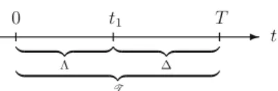
t {t∈T|x(t)=x1, v(t)=0}. (1b) Then,≡ [0, t1]denotes the agent’stravelling period; and ≡(t1, T], the resultingharvesting period.6The total time available is then spent on travelling and on harvesting, with the travelling period preceding the harvesting period. This is illustrated in Fig.1.
The stock of the renewable resource (i.e., the biomass) at time t ∈ T is denoted by s(t) ≥ 0. We assume that the resource is growing at rate g(s) with g(0) = 0.
(Subsequently, we will consider the cases of exponential and logistic growth.) Furthermore, harvesting gradually diminishes the stock. The harvest depends on the abundance of the resource, i.e., on the stocks, and on the harvesting effort h(t) ∈ H ≡ [0,h¯] ⊂ R+. Suppose that for a given stock, the yield from harvesting increases in effort;
moreover, effort is more productive the higher the stock.
Specifically, we assume that the harvesting yield equals zero, H = 0, if either the stock or the effort equals zero, i.e., if s = 0 or h = 0. To capture this idea, we follow the familiar Schaefer model (see Schaefer1954) and specify the revenue from harvesting as a bilinear function of effort and the stock:H (t) = qs(t)h(t), whereq is the catchability coefficient, defined as the fraction of the stock harvested per unit of effort. For convenience, we normalise the units of effort and set q = 1. Then, the harvesting yield equals H (t) = h(t)s(t) if the agent’s location is x1, and H (t) = 0 otherwise. With this specification, the harvestingeffortequally represents the harvestingrate, and we thus use the phrases harvesting effort and harvesting rateinterchangeably.7Putting pieces together, the resulting growth of the stock is governed by the differential equation
˙
s(t)=g(s(t))−h(t)s(t)1(t), ∀t ∈T, s(0)=s0. (1c)
6Once the agent has reached locationx1, they will never start travelling again, and thus the agent completes the planning period at locationx1, i.e.,x(t )=x1,∀t∈ [t1, T].
7The assumption that the agent chooses the harvestingrateh=H /s is justified by the idea of stock-dependent harvesting effort, where the yield from a given amount of effort depends on the abundance of the resource; harvesting effort is then similar to fishing by nets, which captures afractionof the fish stock. If we departed from that view and instead assumed that the agent may choose the harvestingamount Hdirectly, this would affect the dynamics of the optimally controlled system. We are very grateful for a referee for pointing this out.
Fig. 1 Structure of the planning periodT: the travelling period ends when the harvesting period starts at the arrival timet1
where1 denotes the indicator function for the harvesting period, i.e., for timest∈.
Travelling and harvesting are both costly. We assume that the harvesting costC(H )is increasing and convex, i.e., C >0 andC ≥0 for allH ∈R+, withC(0)=0. More specifically, we assume that the harvesting cost is linear in total catch, C(H ) = cH = chs, with 0 ≤ c < p.
Then, instantaneous profit from harvesting amounts to (p−c)h(t)s(t)or, more compactly,Mh(t)s(t), whereM≡ p−cdenotes the per-unit profit (mark-up). Also, travelling is associated with some cost, which generically depends on both speed and acceleration:K(v, a)forv∈V anda∈A. We assume that pausing is costless,K(0,0) = 0, that the travelling cost increases with both speed and acceleration, and that acceleration is more costly the higher the speed, i.e., the partial derivatives ofKsatisfyKv≥0, Ka≥0 and Kva≥0.
Let ρ ≥ 0 denote the discount rate of the agent, and letp be the (constant) price of one unit of the harvested resource. The problem for the agent is then to maximise the discounted profit flow consisting of instantaneous revenue net of the harvesting cost and net of the travelling cost for the planning periodT.8 Presupposing that the agent reasonably choosesh(t)=0,∀t ∈anda(t)=0,∀t ∈ (the choicesh(t) >0 fort∈ora(t) >0 fort ∈would be futile actions), we obtain thetravelling cost
J1(a(·), t1)≡ t1 0
e−ρtK(v(t), a(t))dt and theprofit from harvesting
J2(h(·), t1)≡ T t1
e−ρtMh(t)s(t)dt,
where v and x, and hence the arrival time t1, depend on the acceleration path a(·). We henceforth write, with minor sloppiness,a(·) ∈ A andh(·) ∈ H as shorthand notations for the admissible paths (a(t))t∈, a(t) ∈ A and(h(t))t∈, h(t) ∈ H, respectively. Putting the pieces together, letJ (a(·), h(·), t1)≡ −J1(a(·), t1)+J2(h(·), t1),
8In order to simplify the presentation and to focus on the link between the travelling and the harvesting period, we disregard any residual valueφ(s(T ), T )that the agent may receive at the end of the planning period. Still, one can easily take into account a residual value, as the only effect ofφis to modify the transversality condition of the costate variable (see, e.g., L´eonard and Long1992, Theorem 7.2.1).
then the agent’s optimisation problem reads as
{a(·)∈A,h(max·)∈H,t1∈T} J (a(·), h(·), t1)
s.t. (1a), (1b), (1c), v(t)∈V. (1d) The state constraints(T )≥0 is automatically fulfilled due to assumptions g(0) = 0, and H = 0 whenevers = 0;
similarly, the constraintsx(t) =x1andv(t) =0,∀t ∈ are implied by Eq. (1a) and (1c). Thus, those constraints need not be specified explicitly in Eq. (1d).
Decomposition of the problem
In order to solve problem (1), we draw upon the literature of two-stage optimal control problems, notably on the work of Amit (1986), Tomiyama (1985) and Tomiyama and Rossana (1989),9and decompose the intertemporal optimal travelling–and–harvesting problem into two subsequent problems: a travelling and a harvesting sub-problem. In the travelling problemwe choose an acceleration patha(·), and thus the arrival time t1, so as to move from location 0 to locationx1at minimal cost:
{a(·)∈Amin,t1∈T} J1(a(·), t1) s.t. (1a), (1b). (2a) Since the travelling time t1 can be chosen subject to the constraintx(t1)=x1, we face a free-terminal-time problem with a fixed endpoint constraint.
During the travelling period , the resource grows unimpaired until the agent arrives at the locationx1at time t1, when the harvesting period begins. As a consequence, the stock of the resource at the time of arrival, s(t1), represents the solution of the (interim) growth process
˙
s(t) = g(s(t)) with s(0) = s0 for all t ∈ . In this way, the travelling decision determines the initial value of the stock process for the harvesting problem, s1 = s(t1).
Given those parameters, the resulting subsequentharvesting problem becomes choosing a path of the harvesting effort h(·)that maximisesJ2:
{h(max·)∈H} J2(h(·), t1) s.t. (1c), s(T )free. (2b) The fact that the travelling time of the agent also represents the growth time of the resource is the crucial link between the travelling problem (2a) and the harvesting problem (2b).
As a consequence, the agent has to take into account
9These authors provide optimality conditions for two-stage, finite time dynamic optimization problems. An extension to an infinite horizon is provided by Makris (2001); and applications of this theory to two-stage optimal control problems can, for example, be found in Boucekkine et al. (2004), Saglam (2011), Grass et al. (2012), Caulkins et al. (2013), Krawczyk and Serea (2013), Moser et al. (2014), Long et al. (2017), and Seidl et al. (2018).
that a longer travelling time reduces the time left for harvesting, and thus ceteris paribus the resulting yield.
In contrast, a lower speed of travelling makes travelling less expensive and gives the resource more time to grow, thus providing the opportunity for a more abundant harvest at later times. The travelling–and–harvesting problem(1) takes into account these interdependencies between sub- problems (2a) and (2b).
We next derive necessary conditions for an optimal control pair(a∗(·), h∗(·), t1∗), or for short (a∗, h∗, t1∗), by decomposing the original problem (1), i.e., the sequence of interdependent problems, into two standard problems.
We first consider the harvesting problem of the second stage (2b), and then the travelling problem of the first stage (2a), acknowledging that the solution of the second stage depends on the decision in the first stage. Formally, we proceed as follows: Assuming the existence of the optimal switching timet1in the interior of the time interval T, we solve the second–stage problem and calculate the maximised objective functionJ2∗as a function of the initial state s1 and the switching time t1. Then, we derive the optimal control a∗ and the associated optimal switching timet1by solving the travelling problem of the first stage.
Second stage
Given the control time intervaland the initial condition s(t1) = s1, we solve problem (2b) for an admissible optimal controlh∗. This problem is of a standard form and can be solved using the well-known Pontryagin maximum principle (see, for example, Kamien and Schwartz1991).
Using the solution of the second-stage problem, (h∗, s∗), which depends on the starting values s1 and t1, we calculate the maximised objective value J2∗(s1, t1) ≡ J2(h∗(s1, t1), t1). Then, with the help of J2∗, the original problem (1) reduces to thefirst–stage problem:
First stage
Given the constraints (1a) and (1b), we look for an admissible optimal controla∗(·)on and the associated optimal arrival timet1∗∈T such that
{a(·)∈Amax,t1∈T} V (a(·), t1)≡ −J1(a(·), t1)+J2∗(s(t1), t1), (3) where the optimal arrival timet1∗, satisfying (1b), is deter- mined by the acceleration patha∗(·), throught1
0 v(t)dt = x(t1)−x(0) = x1. Sincet1∗ ∈ (0, T )by assumption, this problem reduces to a standard problem with terminal value (or “salvage” value)J2∗, free terminal timet1 and free end points(t1). (For the solution of such a problem, see, for example, L´eonard and Long1992, sec. 7.2 and 7.6)
Second stage: harvesting
We solve the harvesting problem in this section, and then we solve the problem of the first stage in Section “First stage: optimal travelling–and–harvesting policy”. We con- sider two standard specifications for the growth process of the resource: exponential growth in Section “Exponential growth” and logistic growth in Section “Logistic growth”.
Exponential growth is a stark abstraction for most real growth processes, of course, as possible density depen- dence of the growth rate is neglected. The assumption of exponential growth implicitly postulates that possible density dependence of growth becomes effective at popu- lation scales beyond the considered abundances. Logistic growth, though, takes this density dependence explicitly into account. Thus, exponential growth may be a reason- able assumption for low abundances, while logistic growth is more descriptive for high abundances. For these reasons, both processes should be considered as complementary.10 Exponential growth
Suppose that the stock of the renewable resource, when left unimpaired, increases at a constant rate: g(s(t)) = s(t).
Since the stock is reduced by the catchH (t) ≡s(t)h(t), it evolves according to the differential equation
˙
s(t)=s(t)−h(t)s(t), s(t1)=s1, ∀t∈. (4a) We abstract from discounting for the moment and set ρ = 0. (We show in Appendix A how our results are affected by the presence of a positive discount rate.) Then, the objective function of Eq. (2b) becomes
{h(max·)∈H}J2(h(·), t1)= T
t1
Mh(t)s(t)dt s.t.(4a), s(T )free.
The Hamiltonian of this problem is given by H=Mh(t)s(t)+π(t)s(t) (1−h(t)).
SinceHis linear in the controlh, we expect that the optimal solution is of thebang–bang type, withhjumping between the lower and the upper bound, 0 andh. We now show that¯ such a policy is in fact optimal. To this end, let σ (t) ≡
∂H/∂h = (M−π(t))s(t)denote the switching function.
Then, the maximum principle yields h(t) =
⎧⎨
⎩
0 ifσ (t) <0,
[0,h¯] ifσ (t)=0, ∀t ∈, h¯ ifσ (t) >0,
(4b)
˙
π (t) = h(t)π(t)−Mh(t)−π(t), ∀t∈, (4c)
10Similar models can be found, for example, in the textbooks of Conrad and Clark (1987), Hocking (1991), and Clark (2010).
along with Eq. (4a) and the transversality conditionπ(T )= 0.11Thus the optimal strategy depends on whetherπ is less or greater than M. Next, using π(T ) = 0 together with h(t)= ¯hforπ(t) < M, Eq. (4b) implies that we cannot end the harvesting periodwithh=0. Hence, the agent must complete the harvesting period by harvesting at maximal effort, i.e.,h(T )= ¯h.
Moreover, the solution of Eq. (4c) must satisfy π(t)=
⎧⎪
⎨
⎪⎩
A0e−t ifh(t)=0
M h¯
h¯−1+A1et(h¯−1) ifh(t)= ¯h.
Neither solution achieves the critical valueπ = M more than once. Consequently, there is a unique switching point τ,12implying that we either have (i)h(t)= ¯hfor allt∈, or (ii)h(t) = 0 for allt1 ≤ t < τ andh(t) = ¯h for all τ ≤ t ≤ T. Then, along any path withh = ¯h, the costate variable is given by
π(t)=M h¯ h¯−1
1−e(1− ¯h)(T−t) (5) where we used the transversality condition π(T ) = 0 to determine the constantA1=Mhe¯ T (1− ¯h)/(1− ¯h). Moreover, the switching timeτ is defined by π(τ ) = M so that we obtain from Eq. (5)
τ =T −δ, with δ ≡logh¯
h¯−1. (6)
Since δ is a positive, decreasing and convex function for all values ofh,¯13 we conclude that the larger the maximal harvesting (or effort) rateh, to which we subsequently also¯ refer to as harvesting capacity, the longer the agent can wait and let the resource grow unimpaired in order to allow for more intense harvesting later. Depending on the sign of τ−t1, or equivalently, on the length of the harvesting period, either of two cases may occur (see Fig.2):
Case A:T < δ+t1
In this case, the maximal harvesting rate is relatively low, requiring a longer period of harvesting. There is thus no
11The use of the transversality conditionπ(T )=0 requires thats(T ) is free. Of course,s(T )is required to be non-negative, so that, in principle,π(T )might be positive ifs∗(T ) =0. However, it follows from the exponential growth function (4a), that if the resource is
“heavily depleted” continuously, in the sense thath(t ) > 1 for all t ≥ξ, for someξ > 0,s(t )converges to zero fort → ∞. Hence, while, depending on the parameter choice, the residual stocks(T )may be small, the resource never becomes extinct for any finite timeT, irrespective of the parameter choice.
12Alternatively, this observation follows from Eq. (4c), which implies that evaluated at a switching pointτ, we haveπ (τ )˙ = −M since π(τ )=Mby definition.
13Forh¯=1 we defineδ=1 so as to makeδa continuous function of
¯
h. To see that, in fact, limh¯→1δ(¯h)=1 apply l’Hˆopital’s rule.
time for “waiting” and choosing a zero harvesting rate for some initial time period. Rather, upon arrival the agent immediately begins harvesting (at the maximal rate), so that there is no policy switch during the harvesting period, but maximal harvesting throughout.
Proposition 1 LetT < δ+t1andh¯ =1. Then the optimal harvesting policy is given by
h(t) = ¯h, s(t)=s1e(1− ¯h)(t−t1)
, π(t) = M h¯
h¯−1
1−e(1− ¯h)(T−t) , (7a) for allt∈, and the resulting maximised profit amounts to J2A∗ (s1, t1)≡s1M h¯
h¯−1
1−e(1− ¯h)(T−t1)
. (7b)
Proof The result follows from the preceding analysis.
Case B:T > δ+t1
In this case, the maximal harvesting rate is relatively high, so that the agent can afford to postpone the start of harvesting. Then, after some idle time—or “waiting” time—
has elapsed, harvesting takes place at maximal capacity.
During “the waiting period”, [t1, τ ), the stock is left unimpaired and is thus given by s(t) = s1et−t1, so that at the switching time τ the stock amounts to s(τ ) = s1eτ−t1, which then is the starting value of the stock for the harvesting period[τ, T]. Consequently, for timest ∈ [τ, T] the stock equals
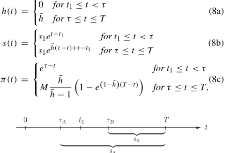
s(t)=A2e(1− ¯h)t =s(τ )e(1− ¯h)(t−τ )=s1eh(τ¯ −t )+t−t1. Proposition 2 LetT > δ+t1andh¯ =1. Then the optimal harvesting policy is given by
h(t) =
0 fort1≤t < τ
h¯ forτ ≤t≤T (8a)
s(t) =
s1et−t1 fort1≤t < τ
s1eh(τ¯ −t)+t−t1 forτ ≤t ≤T (8b) π(t) =
⎧⎨
⎩
eτ−t fort1≤t < τ
M h¯ h¯−1
1−e(1− ¯h)(T−t) forτ ≤t≤T ,(8c)
Fig. 2 Case A: early switching timeτ, i.e., a small harvesting period T−t1< δ; Case B: late switching timeτ, i.e., a large harvesting period T−t1> δ
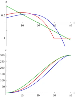
Fig. 3 Optimal harvesting effort in Case B,T > δ+t1: withh¯ =3/2 >1 and thusτ =0.5224 (left diagram), andh¯ =3/4 <1 and thus τ=0.1826 (right diagram), both fort1=0,T=4/3 andM=1; with the stock in green, the costate in blue and the control in red
for allt ∈, and the maximised profit amounts to J2B∗ (s1, t1) ≡ M h¯
h¯−1s1eτ−t1
1−e(1− ¯h)(T−τ )
= Ms1h¯1/(1− ¯h)eT−t1. (8d)
Proof The result follows from the preceding analysis.
Remark 1 ForT =δ+t1, or equivalently, forτ =t1Case A and Case B coincide.
The case ofh¯ =1
Finally, the optimal policy for the caseh¯ =1 is obtained by taking the limits of Case A and Case B:
Remark 2 Ifh¯=1, the optimal profit amounts to J2∗|h¯=1(s1, t1)=
s1M(T −t1) ifT ≤δ+t1
s1MeT−t1−1 ifT > δ+t1.
Discussion
There is a critical length of the harvesting period given by δ =log(¯h)/(h¯−1). If there is plenty of time in the sense thatT −t1 > δ, there is no harvesting during the initial phase[t1, τ )of the harvesting period, but harvesting takes place at the maximum rateh¯ during the final phase [τ, T] of the harvesting period only. In this case, the harvesting technology is so efficient that the agent may wait to let the resource grow further, until harvesting begins. If, however, there is not enough time available, i.e., T −t1 ≤ δ, the agent is required to harvest at the maximum rate throughout.
The relatively low efficiency of the harvesting technology lets the agent harvest as much as possible during the entire harvesting period. Finally, whether the stock increases or decreases during the harvesting process depends on whether the harvesting capacityh¯exceeds or falls short of the growth rate of the stock, which is assumed to be equal to unity here.
The situation when h >¯ 1 is depicted in the left diagram of Fig.3, and whenh <¯ 1, in the right diagram (both for t1=0).
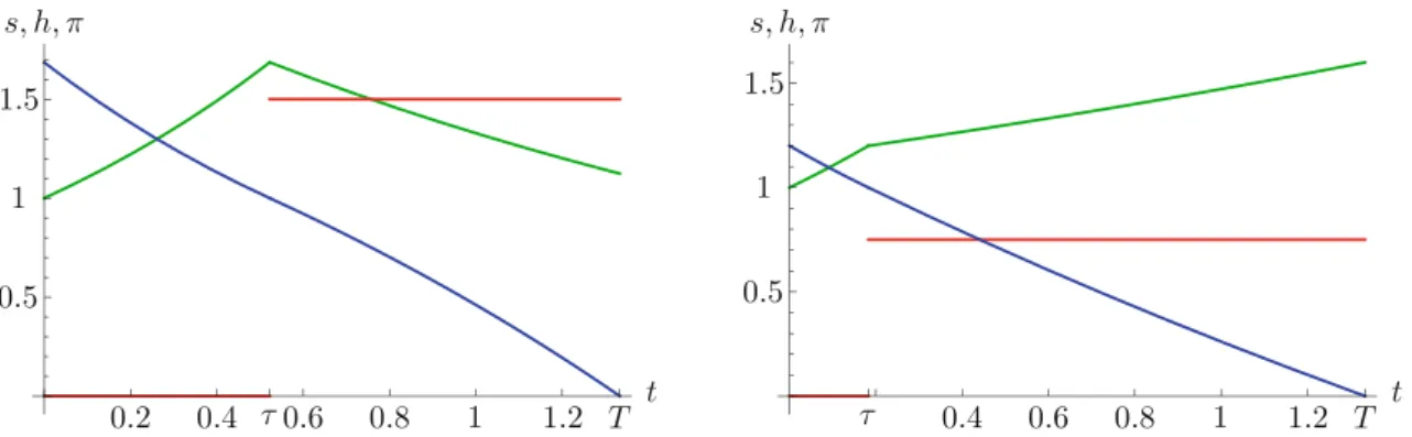
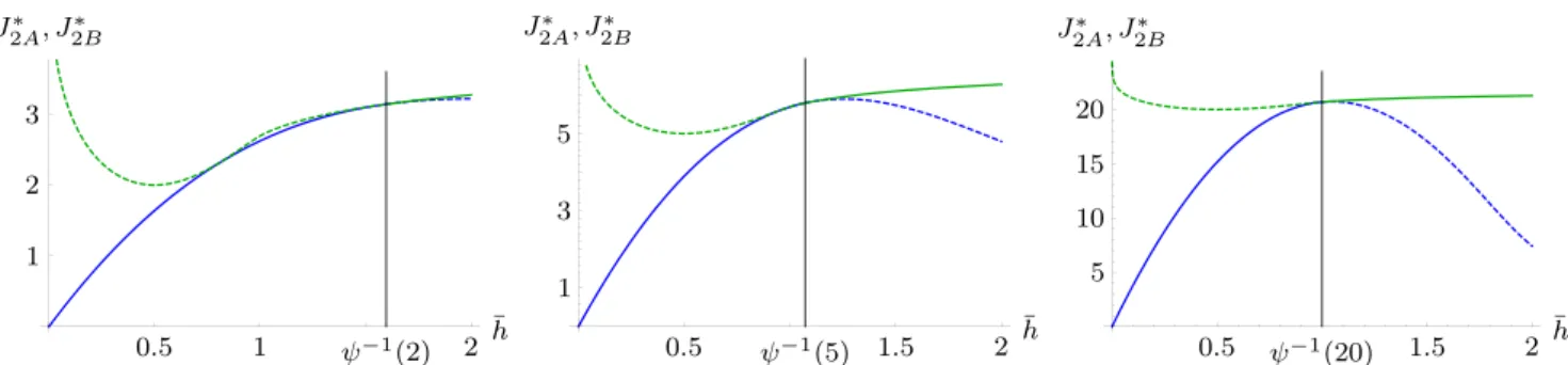
Fig. 4 Maximised profit (solid curves) as a function of the time hori- zon T: forh¯ = 3/4 < 1, thus δ = 4 log(4/3) = 1.1507 (left diagram), and forh¯ =3/2 >1, and thusδ =2 log(3/2)=0.8109
(right diagram): both fort1 = 0 andM = 1. SinceJ2A∗ (in blue) is defined only forT ≤δ, andJ2B∗ (in green) is defined only forT > δ, the dashed parts are merely hypothetical.
Remarkably, the critical length of the harvesting period, δ, depends on the harvesting capacityh¯but is independent of the time horizon; the maximised profit though (in both Case A and B) does depend onT. For any given values of the arrival timet1and the stock at arrivals1, we find that the profit in Case B is higher than or equal to the profit in Case A, i.e., J2B∗ ≥ J2A∗ . This is quite intuitive as a high harvesting capacity is beneficial, allowing for a greater flexibility of the harvesting profile. This is depicted in Fig.4 for the caset1=0. Therein, the vertical line represents the critical timeT =δ+t1for a given value of the harvesting capacityh, and the red curve depicts the (composed) profit¯ function for varying values ofT. If time is scarce in the sense thatT −t1 < δ, Case A applies and the blue curve represents the resulting maximised profit (coinciding with the red curve for valuesT < δ). If there is plenty of time, in the sense thatT > δ+t1, Case B applies and the green curve represents the resulting maximised profit (similarly coinciding with the red curve for valuesT > δ+t1).
Logistic growth
In this section, we modify the growth process of the resource and now explicitly take into account possible density dependence of the growth function. To this end, we assume that the stock obeys a logistic growth process:
g(s(t))=2s(t)
1−s(t) 2
, ∀t∈,
with a carrying capacitys∗ = 2.14 With this specification, the net growth of the stock is governed by the differential equation
˙
s(t)=g(s(t))−h(t)s(t)=s(t) (2−s(t)−h(t)) , ∀t∈. (9a) We assume that the resource has been left unimpaired for a sufficiently long time, or even represents a pristine stock (a scenario that is, for example, also considered by Robinson et al.2008), so that at the arrival timet1the stock equilibrates at its steady state level s(t1) = s∗ = 2.15
14This specification is used, for example, in Pindyck (1984), Conrad and Clark (1987), Thieme (2003), Da Lara and Doyen (2008), Polasky et al. (2011) and other applications. We assume a growth rater=2, which may seem high. The numerical results depend on the ratio of the growth raterand the harvesting capacityh, with a relatively high (low)¯ growth rate resulting in a higher (lower) final stock. However, since the stock never gets fully depleted by timeT(see fn. 11), the particular value of the growth rate does not affect the qualitative results.
15Clearly, in finite time the stock cannot fully recover so that the assumptions(t1) equals the steady state stock s∗ = 2 should be understood as an approximation, unless the stock is actually pristine.
If we assumed instead thats(t1)=s0for some values0∈(0,2), we may have obtained additional cases, namely cases where the agent first refrains from harvesting in order to let the stock grow for some time, and then starts harvesting later.
The remaining model is adopted from Section “Exponential growth”.
The Hamiltonian of the problem is given by H=Mh(t)s(t)+π(t)s(t) (2−s(t)−h(t)).
As in the case of exponential growth, H is linear in the control h. Yet here, as we will see, the optimal solution is not only of the bang-bang type, but may also follow a singular path for some time interval if there is plenty of time (or, equivalently, ifh¯is sufficiently large). To this end, letσ (t)≡∂H/∂h =(M−π(t))s(t)denote the switching function. Then, the maximum principle yields
h(t)=
⎧⎨
⎩
0 ifσ (t) <0,
[0,h¯] ifσ (t)=0, ∀t∈, h¯ ifσ (t) >0,
(9b)
˙
π (t)= −Mh(t)−π(t) (2−2s(t)−h(t)) , ∀t∈, (9c) together with Eq. (9a) and the transversality condition π(T )=0. If we haveσ (t)=0 for some time interval, then the optimal solution contains a singular arc, otherwise we have a bang-bang solution. The next lemma helps to find the specific pattern of the solution.
Lemma 1 π(t1) < M.
Proof See AppendixB.
It follows from Lemma 1 that the optimal policy rule coincides with the rule obtained for exponential growth of the resource (4b): Sinceπ(t1) < M, the optimal path begins with maximal harvesting h(t1) = ¯h. Intuitively, since the initial stock equals its maximum level,s(t1)=2, there is no reason to begin with moderate harvesting or even to wait. If time is scarce, relative to the harvesting capacity, the choice of the maximal harvesting efforth(t)= ¯his optimal for all t ∈ . If, however, there is plenty of time, it is optimal to reduce harvesting in an intermediate time interval, because otherwise harvesting will be completed too early, and the terminal condition that a (marginal) unit of the stock is worthless at the end of the planning horizon,π(T )=0, will not be met.
Proposition 3 The optimal harvesting policy is given by
h(t) = ¯h if h¯≤ ¯hc (10a)
h(t) =
⎧⎨
⎩
h¯ t1≤t < t2,
1 t2≤t < t3, if h >¯ h¯c, h¯ t3≤t < T ,
(10b) with some critical harvesting capacityh¯c >1(depending onT).
Proof See AppendixB.
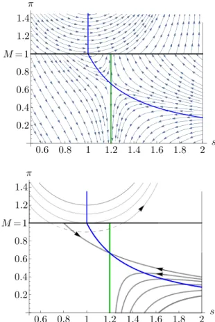
Figure 5 illustrates the two situations characterised in Proposition 3. The left column of the diagrams shows the situation for a low harvesting capacity, while the right column displays the situation for a high harvesting capacity.
In each case, the green curve represents the zerocline of s, while the blue curve represents the zerocline of π. The horizontal line atπ=Mis the switching manifold defining the singular path of the optimal control (see Eq.9b). Since the zerocline ofsis vertical ats=2− ¯h, while the zerocline ofπ reaches the switching manifold ats = 1, both curves have a point of intersection if, and only if, h <¯ 1 (see left column of diagrams). In this case, a saddle path from s0 = 2 to the unique positive steady state (s∞, π∞) = 2− ¯h,h/(2¯ − ¯h)
exists. However, this path is not optimal, since the steady state cannot be reached in finite time.
Consequently, the optimal path starting froms(t1)=2 lies beneath the saddle path terminating atπ(T )=0 according to the transversality condition. In the lower left diagram the optimal trajectories are drawn for different values ofT.
When h >¯ 1, see right column of diagrams in Fig. 5, the zeroclines ofsandπ do not meet, so that in this case a critical trajectory, i.e., a trajectory passing through the point(1,M)=(1,1)exists (see the proof of Proposition 3).
The optimal path, starting froms(t1) =2 and terminating at π(T ) = 0, lies either beneath the critical trajectory or coincides with it, depending on the harvesting capacity (viz. on the time being available for harvesting). The first case applies ifh <¯ h¯c, the latter ifh¯≥ ¯hc. The next lemma characterises the critical harvesting capacityh¯c, and shows that it depends inversely on the time horizonT.
Lemma 2 Letψ:(1,2] →R+be defined by h¯ →ψ(¯h)≡t1+ 1
2− ¯hlog h¯
2(¯h−1)2
(11) with > 0, <0and >0. Then, given timeT, the critical harvesting capacityh¯c is defined as the solution of T = ψ(h), i.e.,¯ h¯c ≡ ψ−1(T ). Equivalently, given some
Fig. 5 Phase diagrams (top) and optimal trajectories (bottom) forh¯= 0.8 (left column) and for forh¯=1.5 (right column). Bold curves show the optimal trajectories (for different values ofT), the thin curves show the trajectories forh=0. The dashed curves represent sub-optimal tra- jectories, i.e., trajectories that violate Eq. (9b). Blue and green curves
display the zeroclines ofπ ands, respectively. The trajectory pass- ing through the point(1,1), displayed in red, represents thecritical trajectory; for this trajectory to exist, the harvesting capacity must be sufficiently large, i.e.,h≥ ¯hc
harvesting capacityh, the critical length of the harvesting¯ period is defined byTc≡ψ(h).¯
Proof See AppendixB.
The intuition for the optimal strategy characterised in Proposition 3 and the critical length of the harvesting period given in Lemma 2 is as follows: In the case T > Tc, there is too much time for harvesting, implying that if the agent followed the critical path (the red path in the right diagram of Fig.5), the terminal condition, i.e., theπ = 0 line, would be reached too early. Because of this, one might consider following a trajectory lying above the critical one, and thus reaching theπ = M line at some stock s > 1.
Then however, since the conditionπ =Mrequires a policy change, one has to dispense with harvesting, and thus to switch toh=0. Yet, dispensing with harvesting implies that the stock increases so that the policy is bound to follow an upward-sloping trajectory (a thin path in the right diagram of Fig. 5), implying that both the stock and the costate variable increase; but this makes it impossible to meet the terminal conditionπ(T ) = 0. For that reason, the optimal policy is as follows: Pursue the critical path by harvesting at the capacity limit until the resource is sufficiently reduced and the point(s, π ) = (1, M)is reached, which happens at timet2. Then, upon arrival at(s, π ) = (1, M), reduce harvesting to the “moderate” effort levelh = 1, which, in view of Eq. (9a) and c, renders both the stock s and its shadow priceπ constant (singular path). This is because unity is the natural growth rate of the resource so that harvesting at exactly this rate represents the sustainable harvesting policywhere the stock level is fully preserved.
Finally, to complete the optimal path, resume harvesting at the maximal rate so as to arrive at the terminal condition π=0 at timeT.
Remark 3 More generally, for an arbitrary growth rate r and an arbitrary carrying capacityK, the zerocline ofs is vertical ats = K
1−hr¯ and the zerocline ofπ is given bys(t)= K2
1+h(t )(Mrπ(t )−π(t )) . Hence, ifh/r¯ approaches unity, the zerocline ofsbecomes vertical ats=0. However, the zerocline ofπ meets the switching manifold, i.e., the horizontal π = M, at s = K/2, irrespective of the values ofh¯ andr. Since the critical trajectory exists for all parameter values, the minimal stock remaining at timeT is determined by the final stocks(T )on the critical trajectory.
Consequently, the final stock may become small but does not converge to zero.
Case A: Eitherh¯ <1 or 1<h¯ <2 andT ≤Tc
In this case, the maximal harvesting effort, relative to the length of the harvesting period—or, equivalently, the length
of the harvesting period, relative to the maximal harvesting capacity—is low, h <¯ h¯c = ψ−1(T ), so that maximal harvesting at rate h, can be maintained throughout the¯ complete harvesting period. Then, the optimal harvesting strategy is given by:
Proposition 4 Let eitherh <¯ 1or1<h <¯ 2andT ≤Tc. Then the optimal harvesting policy is given by
h(t)= ¯h, s(t)= 2h¯−2 he(¯ h¯−2)(t−t1)−2, π(t)=M h(s(T )¯ −s(t))
2s(t)−s(t)2− ¯hs(t),
(12a)
for allt∈, and the resulting maximised profit amounts to J2A∗ (t1)= ¯hM
T t1
s(t)dt= ¯hMlog
2e(2− ¯h)(T−t1)− ¯h 2− ¯h
. (12b) Proof We know from the proof of Proposition 3 that for all sub-critical casesT < Tc (orh <¯ h¯c) defined in Eq. (11), we have h(t) = ¯h for allt ∈ . Substituting this, jointly with initial conditions(t1)= 2 and the terminal condition π(T )=0, into Eq. (9a)–(9c) we obtain Eq. (12a).
Remark 4 For the limiting case whenh¯ → 1, the resulting profit amounts toJ2A∗ |h¯=1(t1)=Mlog
2eT−t1−1 . Remark 5 In the critical case, i.e., whenT =Tc, the optimal profit amounts to
J2Ac (t1)=2¯hMlog h¯
h¯−1
. (13)
Case B: 1<h¯ <2 andT >Tc
In this case, the time available for harvestingT −t1is too long such that, given the maximal harvesting capacity,h, it¯ is not optimal to harvest at the maximal rate all the time, as this implies that the terminal conditionπ =0 is metbefore the final time T. Thus, harvesting cannot be maintained at the maximal rate h¯ throughout the complete harvesting period, but must be reduced for some time interval.
Proposition 5 Let1<h <¯ 2andT > Tc. Then the optimal harvesting policy is given by
h(t)=
⎧⎪
⎨
⎪⎩
¯
h t1≤t < t2, 1 t2≤t < t3, h¯ t3≤t < T ,
(14a)