Multiparticle correlations in complex scattering and the mesoscopic Boson Sampling problem
Juan-Diego Urbina, Jack Kuipers, Quirin Hummel, and Klaus Richter Institut f¨ur Theoretische Physik, Universit¨at Regensburg, D-93040 Regensburg, Germany
We consider the many-body scattering of non-interacting identical particles in mesoscopic chaotic cavities. A complete enumeration of all interfering paths allows us to discriminate single-particle effects from many-body interference due to quantum indistinguishability. In the thermodynamic limit of large particle number massive quantum interference results in a macroscopic, coherent manifestation of many-body correlations. We also incorporate mesoscopic dephasing, present even when the particles scatter simultaneously. Under further simplifications characteristic for optical scenarios, our methods can be used to address open issues related to the Boson Sampling problem.
PACS numbers: 03.65.Sq, 05.45.Mt, 42.50.Ar, 73.23Ad
In quantum mechanics, the symmetrization postulate makes it impossible to characterize systems of identical particles by labeling their constituents individually: iden- tical particles are indistinguishable and their very iden- tity is then affected by quantum fluctuations and inter- ference effects. In open (scattering) systems, where one is interested in processes connecting incoming to outgoing states describing several particles, the transition proba- bilities are given by a mixture of Single-Particle (SP) and Many-Body (MB) effects. By definition, the former are already present in the wave scattering of a single parti- cle, while MB effects are due to interparticle forces and quantum indistinguishability. Remarkably, and in sharp contrast with interactions, indistinguishability does not have a classical limit, and therefore its observable con- sequences provide a hallmark of genuine quantum MB coherence.
A prominent type of MB correlations is exemplified by the celebrated Hong-Ou-Mandel (HOM) effect [1], by now the standard indicator of MB coherence in quantum optics. There, the probability of observing two photons leaving simultaneously in different arms of a beam split- ter is measured. As a function of the delay between the arrival of the incoming photons into the beam splitter, the coincidence probability shows a characteristic dip in agreement with theoretical expectations [1]. The study of MB correlations due to indistinguishability has been a focus of intense scrutiny, with a wealth of hallmark ex- perimental studies of MB scattering of identical particles that have attempted to leave the classic HOM scenario by increasing the number of particles and/or the com- plexity of the scattering process [2–6]. So far, however, theoretical approaches have assumed that already at the SP level the scattering process is itself perfectly known and independent of the characteristics of the incoming state [7–13]. In the mesoscopic scenario depicted in Fig. 1 where the scattering region Ω is a physical cavity, how- ever, this is not the case as the SP scattering process strongly depends of the cavity’s geometry and the energy of the incoming particles. Moreover, a generic cavity is
...
...
...
... 2s
a(j) a(1)
a(N2)
b(j) b(1)
b(N2) Ω
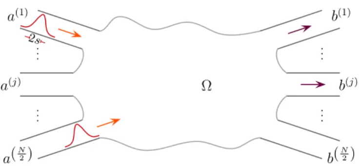
FIG. 1. Many-body scattering of non-interacting indistin- guishable particles. Identical wavepackets with shifted mean position along the leads are scattered by the irregular cavity.
non-integrable, and the mesoscopic MB scattering prob- lem is naturally described within a statistical approach.
In this paper we present analytic results on properties of MB correlations in the mesoscopic regime. Supported by the universal correlations of SP scattering matrices [14] responsible for characteristic mesoscopic effects like weak localization [15] and universal conductance fluctu- ations [16], here we address the emergence of univer- sal MB correlations due to the interplay between clas- sical ergodicity, SP interference and quantum indistin- guishability well beyond standard semiclassical SP pic- tures [17]. Surprisingly, and despite their intrinsically non-classical character, MB correlations are here success- fully explained and computed within a semiclassical ap- proach in terms of interfering SP classical paths in the spirit of the Feynman path integral [18] by providing a one-to-one correspondence between MB classical paths (illustrated in Fig. 2) and terms of the expansion of the MB scattering probabilities. Our complete enumeration and classification of the MB paths allows for an explicit analysis of emergent phenomena in the thermodynamic many-particle limit, something out of reach of leading- order random matrix techniques [19–21]. Moreover, we show that the cavity’s dwell time, a physical parameter characteristic of the mesoscopic regime, drastically af-
arXiv:1409.1558v1 [quant-ph] 4 Sep 2014
fects the HOM effect leading eventually to a universal exponential profile.
Although we present results for both massive bosons and fermions scattered by cavities including all SP and MB interference mechanisms, our methods can be readily extended to the optical case by both using the dispersion relation for photons and neglecting mesoscopic SP effects.
To make connection to corresponding experiments [7–
13] this amounts to replace the cavity Ω by a multi-port waveguide network. Then one finds that the dependence of the MB transition probabilities on the SP scattering matrixσis of purely combinatorial origin. Aaronson and Arkhipov proved that already in this simplified limit, the complexity of this dependence for a given fixedσsuffices to make the calculation of MB transition probabilities a computationally hard task, the so-called Boson Sampling (BS) problem [22]. Our results shed light on timely ques- tions like the thermodynamic limit of BS and show the dynamical origin of the uniform distribution in Hilbert space, an object of ubiquitous presence in BS and re- lated problems like the Bosonic birthday paradox [23].
The set up of the mesoscopic many-body scattering problem is depicted in Fig. 1. The incoming particles (i= 1, . . . , n) with positions (xi, yi) occupy single-particle states represented by normalized wavepackets
φi(xi, yi)∝e−ikixiXi(xi−zi)χai(yi). (1) The longitudinal wavepacket Xi(xi−zi) of theith par- ticle has variance s2i, mean initial position zi si, and approaches the cavity Ω with mean momentum
~ki = mvi > 0 along the longitudinal direction −xi. The transverse wavefunction in the incoming channel ai∈ {a(1), . . . , a(N/2)} isχai(yi) and has energyEai. Al- though a general treatment is possible, we will assume that, except for their relative positions parametrized by zij = zi −zj, the wavepackets and initial transversal modes are identical: si=s, ~ki=~k=mv, andEai= Ech for alli.
The joint probability to findnparticles leaving in chan- nelsb= (b1, . . . , bn) with energiesE= (E1, . . . , En), after entering the cavity in channels a= (a1, . . . , an) is given by
Pa,b= Z ∞
Ech
|Aa,b(E)|2dE1. . . dEn, (2) in terms of theE-dependentn-particle amplitude [24]
Aa,b(E) =
n
Y
i=1
e−i(k−kch(Ei))zi p
~vch(Ei)
X(k˜ −kch(Ei))σbi,ai(Ei). (3) When n = 1, Eq. (3) formally defines the SP scatter- ing matrixσb,a(E) connecting the incoming and outgoing channels a and b. We also have ~kch(E) = mvch(E) = p2m(E−Ech) and ˜X(k) = (1/√
2π)R∞
−∞e−ikxX(x)dx.
Note that the transition probability for distinguishable particles, Pa,b, is insensitive to the relative positions of the incoming wavepacketszij.
If the particles are identical, quantum indistinguisha- bility demands their joint state to be symmetrized ac- cording to their spin [25]. Introducing =−1 (+1) for fermions (bosons), the symmetrized amplitude is given by a sum over then! elements P of the permutation group,
A()a,b(E) =X
P
PAa,Pb(PE). (4) We further introduce
Z <
dE(·) = Z ∞
Ech
dE1
Z E1 Ech
dE2. . . Z En−1
Ech
dEn (·), (5) to avoid the double counting implicit in the identification of the many-body states |E,ai and |PE,Pai. For sim- plicity, in Eq. (5) we assumed that the output channels are open if the incoming are,Ebi ≤Ech. Then
Pa,b() = Z <
|A()a,b(E)|2dE=Pa,binc+Pa,bint, (6) defines the MB transition probability that is naturally separated into an incoherent contribution
Pa,binc =X
P
Z <
|Aa,Pb(PE)|2dE, (7) and a MB term due to interference between different dis- tinguishable MB configurations
Pa,bint = 2n!< X
P6=id.
P Z <
dEAa,Pb(PE)A∗a,b(E). (8) The later depends on the offsetszij that allow for tuning the strength of the interference through dephasing, and thereby can be heuristically understood as sensitive to the degree of indistinguishability itself [5, 6].
The original HOM scenario [1] corresponds to N = 4, n= 2 andσenergy independent. We get
Pa,bHOM16=b2 =|Per(σ)|2+ 1
4 +|Per(σ)|2−1
4 F2(z12) (9) using Eqs. (4) and (6), with Per denoting the permanent (unsigned determinant), and the overlap integral
F(z) = Z ∞
−∞
X(x)X(x−z)dx . (10) Individual σ-matrices with specific entries leading to Eq. (9) and its many-particle generalizations are rou- tinely constructed in arrays of beam splitters connect- ing waveguides for photonic systems [8, 9, 12, 13] and through quantum point contacts for electrons occupy- ing edge states [26, 27]. If the beam splitter or point
(a) ...
...
(b) ...
...
(c) ...
...
(d) ...
...
(e) ...
...
(f) ...
...
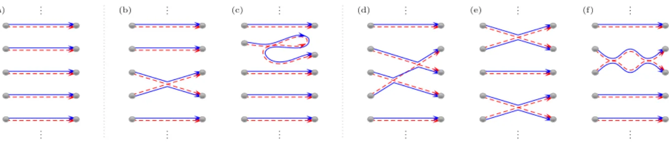
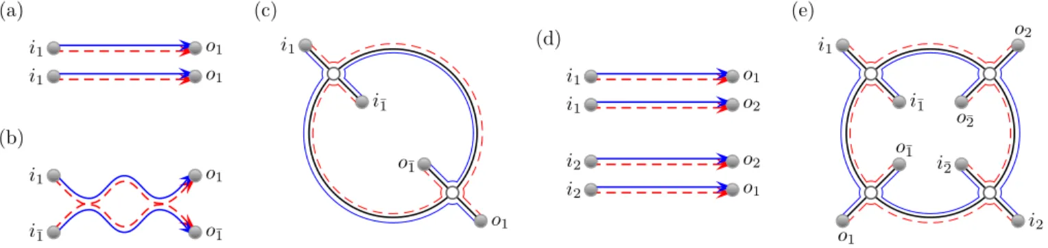
FIG. 2. Many-body (MB) paths contributing to the single-particle (SP) scattering matrix correlations required for calculating of transition probabilities. In (a), both SP and MB correlations are neglected. In (c), weak localization at the SP level is included. For (b,d,e), and (f) only MB correlations are included. Combined SP and MB effects appear when the links in a MB diagram are decorated with SP loops.
contact is replaced by a mesoscopic cavity, acting as a complex scatter, additional time scales are introduced, and thereby further physical effects enter into the prob- lem. Perfect control ofσis neither feasible, nor necessary to address observables averaged over energy windows or variations of the geometry of the cavity. In the semi- classical regime of short wavelengths it is an established fact that for complex scattering where the classical dy- namics is chaotic, products of the formσb,a(E)σ∗b0,a0(E0) display universal features under average, depending only on the presence or absence of time reversal invariance, denoted as the orthogonal (β = 1) and unitary (β = 2) case [14–16, 28]. Universal interference effects in the scattering probabilities are semiclassically understood in terms of statistical correlations among classical actions [14–16, 29].
From Eqs. (3, 4) the averageh|A()a,b(E)|2iof the tran- sition probabilities over an ensemble of σ-matrices in- volves higher-order correlations and different energies.
Our semiclassical calculation of σ-matrix correlations is depicted in Fig. 2 for the case of interest here where bi 6= bj6=i, bi 6= aj and ai 6= aj for all i, j. A 2n-order correlator ofσ-matrices is given by an infinite diagram- matic expansion with terms that can be visualized as a set of links joining n incoming and outgoing channels.
The classical transition probability,
hPa,bclassi=N−n, (11) is obtained from the trivial topology in Fig. 2(a). In Eq. (11)N is the number of open channels at the mean energyU =mv2/2+Echof the incoming particles. Quan- tum effects at the SP level are generated by adding SP loops to the links, as in Fig. 2(c) and can be evaluated up to infinite order to give
hPa,binci= 1 Nn −
2 β −1
∞
X
l=1
(−1)l Nn+l
n+l l
= (N−1 + 2/β)−n, (12)
thenth power of the SP transition probability [14, 15].
In order to calculate Pint, Eq (8), we must include genuine MB effects characterized by correlations between
different SP paths. With an obvious notation, the first MB diagrams without SP loops depicted in Fig. 2 are labeled by {2} (b), {3} (d), {2,2} (e) while Fig. 2(f) shows the diagram{2} with a loop between 2 particles.
The basic correlator{2}in Fig. 2(b) involving a single pair of correlated paths is [16, 30]
hσbi,ai(Ei)σbj,aj(Ej)σ∗bi,aj(Ej)σb∗j,ai(Ei)i (13)
= 1 N3
~2
~2+τd2(Ei−Ej)2+O(1/N4), where τd is the dwell time, the average time a particle with energy (Ei+Ej)/2 remains within Ω before exiting through the leads. Eqs. (8) and (3) give [31]
hPa,binti{2}=− Nn+1
X
i<j
Q(2)(zij), (14) with the generalization of the overlap integral Eq. (10),
Q(2)(z) = Z ∞
−∞
F2(z−vt)e−
|t|
τd
2τd
dt . (15) The functionsQ(2)determine how the MB correlations decay when the delay times τij = zij/v entering F in- crease. We interpret Eq. (15) as follows: Pairs of in- coming particles that are effectively distinguishable get to interfere if their time delay τij in entering the cav- ity is compensated by the time τd the first particle is held within the mesoscopic scattering region. However, the interference gets weighted by the survival probability e−t/τd/τd of remaining inside the chaotic scatter Ω.
Universality of the dephasing of MB correlations is ex- pected ifτdcompetes with the delay timesτij and widths τs =s/v of the incoming wavepackets. Universal expo- nential tails in the interference profile for|zij| scan be made explicit if we assume that the overlapF(x) decays faster than exponentially to giveQ(2)(zs)∼e−|z|/vτd. As shown in Fig. 3, the region of exponential tails grows with the ratioτd/τs. We can thus identify a universal regime where the suppression of MB interference is ex- ponential
Q(2)(z)−−−−−−−−−→ Cvτdvτs1/k (2) τs
2τd
e−
|z|
vτd , (16)
-5 0 5 10ΤΤs 0.8
0.9 1 XN2Pa,b1¹b2\
exponential ΤdΤs=10 ΤdΤs=2 ΤdΤs=0.1 gaussian
FIG. 3. Overlapping (Gaussian due the shape of the incom- ing wavepackets) and universal (exponential) regimes for the mesoscopic HOM interference profile, depicting the probabil- ity of finding two bosons in different exit channels.
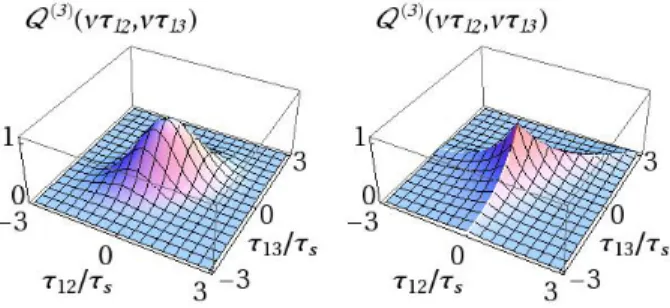
FIG. 4. Transition between the overlapping (τd/τs= 0.1, left) and the universal exponential (τd/τs = 10, right) regime for the three-body interference term, Eq. (18).
with C(2) = s−1R∞
−∞F2(z)dz. In the opposite regime, we observe a non-universal result
Q(2)(z)−−−−−−−−−→ Fvτsvτd>1/k 2(z). (17) Here the interference profile depends, as in the opti- cal HOM effect Eq. (9), on the shape of the incoming wavepackets. These observations are not particular to two-body interference. The diagram Fig. 2(d) containing three-body correlations (the mesoscopic analogue of the correlations measured in [6]) gives
hPa,binti{3}= 2 Nn+2
X
i<j<k
Q(3)(zij, zkj), (18) with regimes shown in Fig. 4 and given by
Q(3)(z, z0)
vτdvτs1/k
−−−−−−−−−→ C(3) e
−3Max(z,z0,0) vτd
2τd
e
z+z0 vτd
2τd ,
vτsvτd>1/k
−−−−−−−−−→ F(z)F(z0)F(z−z0) (19) withC(3)=s−2R∞
−∞F(z)F(z0)F(z−z0)dzdz0.
As the main application however, we address the fate of MB interference effects due to indistinguishability in the thermodynamic limit N, n → ∞, a fundamental is- sue of present interest [2, 22, 23, 32, 33]. The expan- sion of the correlators in powers ofN−1, Eqs. (11,14,18) must be reconsidered in view of the fast (combinatorial)
growth (with n) of the number of MB terms in each diagram. For a well defined thermodynamic limit we need a proper scalingN =αnη to control asymptotically large diagrams. It can be shown order by order [31] that loop contributions are of higher order and the dominant contributions are of the form{2},{2,2},{2,2,2}, . . ., ob- tained by simple pairwise correlations among links. Us- ing Eq. (13), all pairwise diagrams can be evaluated in closed form giving
hPa,binti{2,2}= 2 Nn+2
X
(i,i0)<(j,j0)
Q(2)(zij)Q(2)(zi0j0) (20) and the obvious generalization for arbitrary orders.
We specifically consider now the case zij = 0 where all the particles are injected at the same mean position and where we expect the peak of the interference profile.
All contributions which are not made up from pairs of correlated trajectories vanish forn 1, while from the sum of the pairwise diagrams we easily get
hPa,b()izij=0
hPa,bclassi
−−−→n1 [n/2]
X
l=0
−Q(2)(0) N
l
(2l−1)!!
n 2l
. (21) By inspection of the series we find that the proper scaling giving a finite, non-zero thermodynamic limit must be η= 2, and we obtain finally
hPa,b()izij=0
hPa,bclassi N=αn2
−−−−→n→∞ e−Q(2)(0)/2α. (22)
Equation (22) shows that under ensemble average and a proper scaling, in the universal limit MB interference due to indistinguishability produces macroscopic statisti- cal effects. More importantly, following well established results in the field of quantum chaos [34],it is expected that for Eq. (22) to hold in chaotic systems it is enough to perform averages over small variations of the system parameters. The quadratic scaling N = αn2 has been noted before [22, 32, 33], and it is related with the so- called bosonic birthday paradox [23]. Within our dynam- ical approach it is supported by the conjecture [31]
hPa,b()iτzdij=0=0 hPa,bclassi =
n−1
Y
k=0
N
N+k, (23)
which gives the asymptotics (forη6= 2) hPa,b()iτzd=0
ij=0
hPa,bclassi
! N=αnη
−−−−→n→∞
0 for 1< η <2 1 for η >2, showing a sharp transition between classical and quan- tum correlations in the thermodynamic limit.
Along with the semiclassical techniques in [31], for the case whenzij = 0 the transition probabilities should be
amenable to random matrix approaches which could be a route to proving Eq. (23). Also in [31] we calculate the leading order of the second moment and variance of the transition probabilities. In fact, determining just the leading order of higher moments should be perti- nent for the Permanent Anti-Concentration Conjecture important for BS [22]. Intriguingly then, semiclassical diagrams and random matrices open up new avenues for understanding permanent statistics.
In conclusion, we have presented a semiclassical theory of mesoscopic many-body scattering of non-interacting, identical particles based on interfering single-particle tra- jectories. We have shown the existence of a universal regime where massive interference due to chaotic scat- tering leads to quantum indistinguishability effects that survive in the thermodynamic limit, providing a dynam- ical basis for recent statistical approaches to the Boson- Sampling problem. We also show that if the typical time τda particle remains in the scattering region is finite, the HOM profile universally displays exponential (instead of Gaussian) tails, thus extending the regime where many- body correlations can be detected. Finally, in the limit τd = 0, our methods can be used to describe mode cor- relation functions in random optical arrays where other type of MB correlations can play a role.
We want to thank Andreas Buchleitner and Malte Tichy for instructive discussions, and Markus Birberger for his help in preparing the mansucript.
[1] C. K. Hong, Z. Y. Ou, and L. Mandel,Phys. Rev. Lett.
59, 2044 (1987).
[2] M. Tillmann, B. Dakic, R. Heilmann, S. Nolte, A. Sza- meit, and P. Walther,Nature Photon.7, 540 (2013).
[3] M. A. Broome, A. Fedrizzi, S. Rahimi-Keshari, J. Dove, S. Aaronson, T. C. Ralph, and A. G. White,Science339, 794 (2013).
[4] A. Crespi, R. Osellame, R. Ramponi, D. J. Brod, E. F. Galvao, N. Spagnolo, C. Vitelli, E. Maiorino, P. Mataloni, and F. Sciarrino, Nature Photon. 7, 545 (2013).
[5] Y.-S. Ra, M. C. Tichy, H.-T. Lim, O. Kwon, F. Mintert, A. Buchleitner, and Y.-H. Kim, Nature Commun. 4, (2013).
[6] M. Tillmann, S.-H. Tan, S. E. Stoeckl, B. C. Sanders, H. de Guise, R. Heilmann, S. Nolte, A. Szameit, and P. Walther, Boson Sampling with Controllable Distin- guishabilityarXiv:1403.3433 (2014).
[7] M. C. Tichy, M. Tiersch, F. de Melo, F. Mintert, and A. Buchleitner,Phys. Rev. Lett.104, 220405 (2010).
[8] S. Aaronson and A. Arkhipov, Boson sampling is far from uniform arXiv:1309.7460 (2013).
[9] P. P. Rhode, K. R. Motes, and J. P. Dowling,Sampling generalized cat states with linear optics is probably hard arXiv:1310.0297 (2013).
[10] C. Gogolin, M. Kliesch, L. Aolita, and J. Eis- ert, Boson-sampling in the light of sample complexity
arXiv:1306.3995 (2013).
[11] V. S. Shchesnovich,Phys. Rev. A89, 022333 (2014).
[12] J. B. Spring, B. J. Metcalf, P. C. Humphreys, W. S. Kolthammer, X.-M. Jin, M. Barbieri, A. Datta, N. Thomas-Peter, N. K. Langford, D. Kundys, J. C. Gates, B. J. Smith, P. G. R. Smith, and I. A. Walm- sley,Science339, 798 (2013).
[13] B. J. Metcalf, N. Thomas-Peter, J. B. Spring, D. Kundys, M. A. Broome, P. Humphreys, X.-M. Jin, M. Barbieri, W. S. Kolthammer, J. C. Gates, B. J. Smith, N. K. Lang- ford, P. G. R. Smith, and I. A. Walmsley,Nature Comm.
4, 1356 (2013).
[14] G. Berkolaiko and J. Kuipers,Phys. Rev. E85, 045201 (2012);J. Math. Phys.54, 112103 (2013).
[15] K. Richter and M. Sieber, Phys. Rev. Lett. 89, 206801 (2002).
[16] S. M¨uller, S. Heusler, A. Altland, P. Braun, and F. Haake,New J. Phys.11, 103025 (2009).
[17] See for example R. K. Badhuri and M. BrackSemiclas- sical Physics, Addison-Wesley (Reading) 1997.
[18] L. S. Schulman, Techniques and Applications of Path Integration, John Wiley & Sons (New York) 1981;
M. Gutzwiller,Chaos in Classical and Quantum Mechan- ics, Springer Verlag (New York) 1990.
[19] C. W. J. Beenakker, J. W. F. Venderbos, and M. P. van Exter,Phys. Rev. Lett.102, 193601 (2009).
[20] M. Cand and S. E. Skipetrov,Phys. Rev. A 87, 013846 (2013).
[21] M. Cand, A. Goetschy, and S. E. Skipetrov, Transmis- sion of quantum entanglement through a random medium arXiv:1406.7202 (2014).
[22] S. Aaronson and A. Arkhipov, STOC ’11 43rd ann. ACM Symp. Theo. Comp.333, (2011).
[23] A. Arkhipov and G. Kuperberg,Geom. and Topol. Mon.
18, 1 (2012).
[24] S. Weinberg, The quantum theory of fields Cam- bridge University Press (NY) 2005; M. Gell-Mann and M. L. Goldberger,Phys. Rev.91, 398 (1953).
[25] J. J. Sakurai, Modern Quantum Mechanics, Addison- Wesley (Reading) 1967.
[26] E. Bocquillon, V. Freulon, F. D. Parmentier, J.- M. Berroir, B. Placais, C. Wahl, J. Rech, T. Jonckheere, T. Martin, C. Grenier, D. Ferraro, P. Degiovanni, and G. Feve,Annalen der Physik526, 1 (2014).
[27] C. W. J. Beenakker, C. Emary, M. Kindermann, and J. L. van Velsen,Phys. Rev. Lett.91, 147901 (2003).
[28] C. W. J. Beenakker,Rev. Mod. Phys.69, 731 (1997).
[29] D. Waltner, Semiclassical approach to mesoscopic sys- tems, Springer-Verlag (Heidelberg) 2012.
[30] J. Kuipers and M. Sieber, Phys. Rev. E 77, 046219 (2008).
[31] See supplementary material.
[32] M. C. Tichy, K. Mayer, A. Buchleitner, and K. Molmer, Phys. Rev. Lett.113, 020502 (2014).
[33] V. S. Shchesnovich,Conditions for experimental Boson- Sampling computer to disprove the Extended Church- Turing thesis, arXiv:1403.4459 (2014).
[34] F. Haake, Quantum Signatures of Chaos, Springer (Berlin) 2010.
SUPPLEMENTARY MATERIAL CALCULATION OFQ2(z) Using the definition Eq. (8) we get
Q(2)(z) = Z ∞
Ech
dE1dE2
ei(kch(E2)−kch(E1))z 1 +hτ
d(E1−E2)
~
i2 (24)
× |X˜(k−kch(E1))|2|X˜(k−kch(E2))|2
~2vch(E1)vch(E2) , where the symmetry of the integrand under interchange of E1 and E2 is used. To further proceed, we use Ei =Ech+~2q2i/2m and q= q2−q1, Q = (q1+q2)/2.
Then we observe that the momentum representation of the incoming wavepackets ˜X(qi−k) are strongly localised aroundq1 =q2 =k. As long as ks 1 we can extend the lower limit of integrals to −∞and keep only terms of first order inq. Under this conditions Eq. (24) yields
Q(2)(z) = Z ∞
−∞
dQdq eiqz
1 +v2τd2q2 (25)
× |X˜(Q−k−q/2)|2|X˜(Q−k+q/2)|2, which can be finally transformed into
Q(2)(z) = Z ∞
−∞
F2(z−vt)e−|t|τd 2τd
dt . (26)
SEMICLASSICAL TREATMENT OF SCATTERING MATRIX CORRELATORS Fornbosons, we start with the expression
A˜+n = 1
√n!
X
P∈Sn
n
Y
k=1
Zik,oP(k), (27) where we sum over all permutationsP of{1, . . . , n} and whereZ =σTis the transpose of the single particle scat- tering matrix σ (so we can identify the first subscript as an incoming channel and the second as an outgoing one). For simplicity we assume that all the channels are distinct. This quantity is related to then-particle ampli- tude when the particle energies coincide orτd= 0.
We will treat correlators of An using a semiclassical approach. This is heavily based on [35–38] and we refer in particular to [35, 37] for the underlying details and methods.
Transmission probabilities First we are interested in
|A˜+n|2= ˜A+n( ˜A+n)∗= 1 n!
X
P,P0∈Sn
n
Y
k=1
Zik,oP(k)Zi∗k,oP0(k). (28)
The averages over scattering matrix elements are known both semiclassically and from RMT (see [37, 39] for ex- ample)
Za1,b1· · ·Zan,bnZα∗1,β1· · ·Zα∗n,βn
(29)
= X
σ,π∈Sn
VN(σ−1π)
n
Y
k=1
δ(ak−ασ(k))δ(bk¯−βπ(k)¯ ), where V are class coefficients which can be calculated recursively.
However, since the channels are distinct, for each pair of permutationsP,P0in Eq. 28 only the term withσ=id andπ=P(P0)−1in Eq. 29 contributes. One then obtains the result
P˜n+=h|A˜+n|2i= 1 n!
X
P,P0∈Sn
VN(τ), (30)
whereτ=P(P0)−1is the target permutation of the scat- tering matrix correlator. Sinceτ is a product of two per- mutations, summing over the pairP,P0 just means that τ covers the space of permutationsn! times and
P˜n+= X
τ∈Sn
VN(τ). (31)
Since the class coefficients only depend on the cycle type of τ, one could rewrite the sum in terms of partitions.
For this we let v be a vector whose elements vl count the number of cycles of length l in τ so that P
llvl = n. Accounting for the number of ways to arrange the n elements in cycles, one can write the correlator as
P˜n+ =
P
llvl=n
X
v
n!VN(v) Q
llvlvl! (32) where we represent the argument ofV by the cycles en- coded inv.
Typically, one considers correlators with a fixed target permutation, rather than sums over correlators as here in Eq. 31. For example fixing τ = (1, . . . , n) provides the linear transport moments whileτ =idgives the mo- ments of the conductance. A summary of some of the transport quantities which have been treated with RMT and semiclassics can be found in [38].
Examples
Representing the argument of the class coefficientsVN
instead by its cycle type, one can directly write down the result forn= 1,2:
P˜1+=VN(1)
P˜2+=VN(1,1) +VN(2), (33)
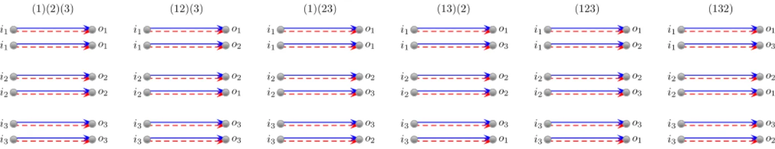
while forn= 3 there are 6 permutations (1)(2)(3) (123) (132)
(1)(23) (12)(3) (13)(2), (34) and so
P˜3+=VN(1,1,1) + 3VN(2,1) + 2VN(3). (35) With the recursive results in [37, 39] for the class co- efficients we can easily find the following results for low n:
Unitary case
Without time reversal symmetry, the results are P˜1+= 1
N P˜2+= 1
N(N+ 1) P˜3+= 1
N(N+ 1)(N+ 2) P˜4+= 1
N(N+ 1)(N+ 2)(N+ 3)
P˜5+= 1
N(N+ 1)(N+ 2)(N+ 3)(N+ 4). (36) The pattern seems to be
P˜n+= Γ(N)
Γ(N+n). (37)
An inductive proof using Eq. 32 and recursive sums for the class coefficients should be possible. The expansion inN−1 would then be
P˜n+= 1
Nn −n(n−1)
2Nn+1 +. . . (38) Orthogonal case
With time reversal symmetry, the results are P˜1+= 1
(N+ 1) P˜2+= 1
N(N+ 3) P˜3+= 1
N(N+ 1)(N+ 5) P˜4+= 1
N(N+ 1)(N+ 2)(N+ 7)
P˜5+= 1
N(N+ 1)(N+ 2)(N+ 3)(N+ 9), (39) suggesting a general result of
P˜n+= Γ(N) Γ(N+n)
(N+n−1)
(N+ 2n−1), (40)
with an expansion of P˜n+= 1
Nn −n(n+ 1)
2Nn+1 +. . . (41) Diagrammatic treatment without time reversal
symmetry
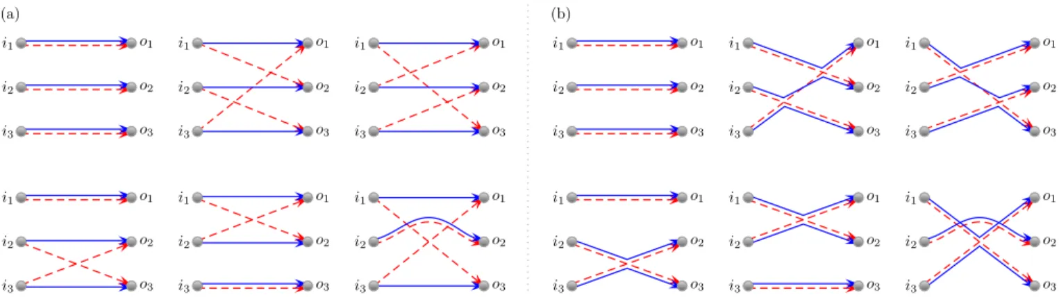
For a given cycle (1, . . . , l) in the target permutationτ the semiclassical trajectories have a very particular struc- ture whereby we first travel along a trajectory with pos- itive action fromi1 too1 and then in reverse back along a trajectory with negative action to i2 and so on along a cycle until we return to i1. For example for n = 3 we have the trajectory connections in Fig. 5(a) for each target permutationτ in Eq. 34.
For the actions of the diagram to nearly cancel, and to obtain a semiclassical contribution, the trajectories must be nearly identical, except at small regions called encounters. By directly collapsing the trajectories onto each other, as in Fig. 5(b) we obtain some of the leading order diagrams for eachτ. In fact for each diagram, fol- lowing the rules of [40], the semiclassical contribution is a factor of−N for each encounter and a factor of N−1 for each link between the encounters. For each cycle of lengthlin the diagrams in Fig. 5(b) one then has a factor of orderN−2l+1. One then needs to generate all permis- sible diagrams.
As shown in [36, 37] however the vast majority of semi- classical transport diagrams cancel. Those which remain can be untied until their target permutation becomes identity. For systems without time reversal symmetry, which we consider first, they can be mapped to primitive factorisations. One can reverse the process to build the diagrams by starting with a set of n independent links and tying together two outgoing channels into a new en- counter. This tying process increases the order of the diagram by N−1. If the outgoing channels are labelled byj and kthen the target permutation also changes to τ(j k). For example going from the top left diagram of Fig. 5(b) tying together any two outgoing channels leads to the three example along the bottom row. The dia- grams correspondingly move from orderN−3to N−4.
Tying the remaining outgoing channel to one of those already tied leads to a diagram of the type further along the top row of Fig. 5(b) [for each of which there are 3 possible arrangements, and an alternative with a single larger encounter] and now of orderN−5.
Of course one could retie the same pair chosen in the first step, so that the target permutation is again identity.
Such a diagram is however not shown in Fig. 5(b) but can be thought of as a higher order correction to a diagonal pair of trajectories. These types of diagrams appear when one treats the conductance variance for example. Such diagrams have a graphical interpretation which we will discuss below and use to generate them.
(a) i1
i2
i3
o1
o2
o3
i1
i2
i3
o1
o2
o3
i1
i2
i3
o1
o2
o3
i1
i2
i3
o1
o2
o3
i1
i2
i3
o1
o2
o3
i1
i2
i3
o1
o2
o3
(b) i1
i2
i3
o1
o2
o3
i1
i2
i3
o1
o2
o3
i1
i2
i3
o1
o2
o3
i1
i2
i3
o1
o2
o3
i1
i2
i3
o1
o2
o3
i1
i2
i3
o1
o2
o3
FIG. 5. (a) The permutations on 3 labels represented as trajectory diagrams. (b) Semiclassical contributions come when the trajectories are nearly identical, as when collapsed onto each other.
Forests
At leading order for each cycle of length l in τ the trajectories however form a ribbon graph in the shape of a tree. The tree has 2l leaves (vertices of degree 1) and all further vertices of even degree greater than 2. Such trees can be generated [41] by first treating unrooted trees whose contributions we store in the generating function f. Using the notation in [35], the function satisfies
f = r N −
∞
X
k=2
f2k−1, f N =
q
1 + 4rN22 −1
2r , (42)
where the power ofrcounts the number of leaves and the encounters may not touch the leads since the channels are distinct. Rooting the tree we add a leave to arrive at the generating functionF =rf while settingr2=swe arrive at
F N =
q
1 +N4s2 −1
2 . (43)
Expanding in powers ofs F = s
N − s2 N3 +2s3
N5 −5s4
N7 +14s5
N9 +. . . (44) one has an alternating sequence of Catalan numbers, A000108 [42].
When summing over all permutations for τ, each cy- cle of length l can be arranged in (l−1)! ways and we now wish to include this factor in the ordinary generating function. First we divide instead by a factor l with the transformation
K0
N = Z F
sN ds= r
1 + 4s
N2 −1 (45)
+1 2ln
N4
1−q 1 + N4s2
2s2 +N2
s
,
so thatK0 becomes the exponential generating function of the leading order trees multiplied by the factor (l−1)!
as required. To now generate any forest of trees corre- sponding to all permutationsτ we can exponentiateK0
to obtain the exponential generating function eK0−1 = s
N +(N−1)s2
2N3 +(N2−3N+ 4)s3 6N5 +(N3−6N2+ 19N−30)s4
24N7 +. . . (46) whose first few terms can be explicitly checked against diagrams.
Higher order corrections to trees
For each given cycle (1, . . . , l) of τ there are higher order (inN−1) corrections which can be organised in a diagrammatic expansion [35, 38]. For systems without time reversal symmetry, the first correction occurs two orders lower than leading order and the corresponding diagrams can be generated by grafting the unrooted trees on two particular base diagrams. Repeating the steps in [35], while excluding the possibility for encounters to touch the leads (since the channels are distinct), one first obtains
K2=−(f2+ 3)f4
6(f2+ 1)3 , (47) where handily, the method for subleading corrections au- tomatically undercounts by a factor of l so we directly obtain the required exponential generating function. Fi- nally we substitute from Eq. 42 and find
12N K2= 1 + N6s2
1 +N4s2
32 −1. (48) The exponential generating function eK0+K2 −1 would then generate all corresponding diagram sets up to this order.
Other corrections
However, the higher order corrections to trees are less important than the higher order corrections to other target permutation structures. For any pair of cycles (1, . . . , k)(k+ 1, . . . , l) inτ we can have diagrams which are orderN−2 smaller than a pair of leading order trees.
For example, tying any two outgoing channels of a tree on the cycle (1, . . . , l) would break the target permutation into two as here.
To generate diagrams with two cycles, we graft trees around both sides of a circle as for the cross correlation of transport moments treated in [35]. This will include the example with n = 3 mentioned at the start of this subsection.
Following the steps in [35], while excluding the possi- bility of encounters touching the lead, one finds the gen- erating function
κ=−ln
1−f12f22 (1−f12)2(1−f22)2
(49) + ln
1 (1−f12)2
+ ln
1 (1−f22)2
,
wheref1 andf2 are thef in Eq. 42 but with arguments r1andr2respectively. The last two terms are corrections for when eitherr1 orr2is 0 to remove diagrams with no trees on either side of the circle. In [35],κwas differen- tiated and such terms removed automatically, but here this correction simplifies the result to
κ=−ln
1−f12f22
. (50)
This generating function again undercounts by both a factor ofkand (l−k) and can therefore be thought of as an exponential generating function of both arguments.
Setting s1 = s2 = s then sums the possible splittings of thel elements into two cycles (along with the combi- natorial factor of choosing the label sets), counting each splitting twice. This then provides the following expo- nential generating function
κ1=−1 2ln
1−f4
(51)
=−1 2ln
"
N4 2s2
r 1 + 4s
N2
1 + 2s N2
−1− 4s N2
!#
,
whose expansion is
κ1= s2 2N4 −2s3
N6 +29s4
4N8 −26s5
N10 +. . . (52)
Order of contributions
With the diagrams treated so far the exponential gen- erating function would be
eK0+κ1+K2−1 = s
N +(N3−N2+N−1)s2 2N5
+(N4−3N3+ 7N2−15N+ 20)s3 6N7
+. . . (53)
and the differences from Eq. 46 occur two orders lower in N−1 than the leading term from independent links.
This is because the additional diagrams required at least two tying operations. However, we wish to know how the contributions change whennscales withN in some way.
First we can compare the contributions coming from K2 to those from K0. In the forest we can replace any tree fromK0with its higher order correction inK2. Since there can be at mostntrees, and the correction is order N−2 smaller, these corrections will be bound bynN−2, up to the scale of the generating function coefficients.
This means that we can expect the contributions from K2 to not be important whenn=O(N2) as we take the limitN → ∞.
Next we compare the contributions coming fromκ1to those from K0. In the forest we can now replace any tree by breaking itsl cycle into two, say k and (l−k).
Alongside the generating function coefficients, the two new cycles come with the factor (l−k−1)!(k−1)! instead of the (l−1)! that was with the tree. Since
1 (l−1)!
X
k=1
l−1 l
k
(l−k−1)!(k−1)!
=
l−1
X
k=1
l
(l−k)k ≤l , (54)
this contribution is bound by nN−1 and should not be important whenn=O(N).
Continuing in this vein we could break up any tree into three cycles and generate those diagrams but this should also be higher order whenn N. Keeping our expansion to this order we should have
eK0+κ1−1 = s
N +(N2−N+ 1)s2
2N4 (55)
+(N3−3N2+ 7N−12)s3 6N6 +. . .
Time reversal symmetry
With time reversal symmetry, additional diagrams be- come possible. For example we may reverse the trajec- tories on one side of the circle used for cross correlations and obtain 2κ1 instead of justκ1. There are also addi- tional base diagrams at the second order correction to
trees, which may be treated as in [35], but which we do not treat here since there are now diagrams at the the first order correction. These can be generated by graft- ing trees around a M¨obius strip. Following again the steps in [35] while excluding the possibility of encounters touching the lead one obtains the generating function
K1=1 2ln
1−f2 1 +f2
, (56)
or explicitly
K1=−1 4ln
1 + 4s
N2
(57)
=− s N2 +2s2
N4 −16s2
3N6 +16s4
N8 −256s5 5N10 +. . . Compared to the leading order forest, we could replace any tree by its higher order correction and obtain a term bound bynN−1, again up to the scale of the generating function coefficients. Restricting to n = O(N) the the exponential generating function would be
eK0+2κ1+K1−1 = (N−1)s
N2 +(N2−3N+ 7)s2 2N4 +(N3−6N2+ 28N−75)s3
6N6
+. . . (58)
Fermions Fornfermions we start instead with
A˜−n = 1
√n!
X
P∈Sn
(−1)P
n
Y
k=1
Zik,oP(k), (59)
where (−1)P represents the sign of the permutation, counting a factor of -1 for each even length cycle in P.
Following the same steps for bosons, one has P˜n−=h|A˜−n|2i= X
τ∈Sn
(−1)τVN(τ), (60)
so for example
P˜3−=VN(1,1,1)−3VN(2,1) + 2VN(3). (61) Calculating the class coefficients recursively one then finds the following results for lown:
Unitary case
Without time reversal symmetry, the results are P˜1−= 1
N P˜2−= 1
N(N−1) P˜3−= 1
N(N−1)(N−2) P˜4−= 1
N(N−1)(N−2)(N−3)
P˜5−= 1
N(N−1)(N−2)(N−3)(N−4), (62) The pattern seems to be
P˜n−= Γ(N−n+ 1)
Γ(N+ 1) , (63)
and the expansion inN−1 would then be P˜n−= 1
Nn +n(n−1)
2Nn+1 +. . . (64) Orthogonal case
With time reversal symmetry, the results are P˜1−= 1
(N+ 1) P˜2−= 1
(N+ 1)N P˜3−= 1
(N+ 1)N(N−1) P˜4−= 1
(N+ 1)N(N−1)(N−2)
P˜5−= 1
(N+ 1)N(N−1)(N−2)(N−3) (65) suggesting a general result of
P˜n−=Γ(N−n+ 2)
Γ(N+ 2) (66)
with an expansion of P˜n+= 1
Nn +n(n−3)
2Nn+1 +. . . (67) Generating functions
However, because our semiclassical generating func- tions are organised by cycle type, we simply need to re- places by −s and multiply the K type functions by -1 appropriately.
(1)(2)(3) i1
i2
i3
o1
o2
o3
i1
i2
i3
o1
o2
o3
(12)(3) i1
i2
i3
o1
o2
o3
i1
i2
i3
o2
o1
o3
(1)(23) i1
i2
i3
o1
o2
o3
i1
i2
i3
o1
o3
o2
(13)(2) i1
i2
i3
o1
o2
o3
i1
i2
i3
o3
o2
o1
(123) i1
i2
i3
o1
o2
o3
i1
i2
i3
o2
o3
o1
(132) i1
i2
i3
o1
o2
o3
i1
i2
i3
o3
o1
o2
FIG. 6. The leading order diagrams for the variance with 3 particles are created by finding semiclassical diagrams with 6 incoming and outgoing channels. When the channels coincide, the leading order diagrams must reduce to separated links corresponding to one of the permutations on 3 labels depicted.
The variance Now fornbosons we look at
|A˜+n|4= 1 (n!)2
X
P,P0 R,R0∈Sn
n
Y
k=1
Zik,oP(k)Zi∗k,oP0(k)
×Zik,oR(k)Zi∗k,oR0(k), (68)
or rather the average L+n =D
|A˜+n|4E
. (69)
However, when we now compare to Eq. 29 such an av- erage involves summing over permutations of length 2n while each of the originally distinct channels appears ex- actly twice. For example
L+1 =hZi1,o1Zi1,o1Zi∗1,o1Zi∗1,o1i= 2VN(1,1) + 2VN(2), (70) since the delta function conditions in Eq. 29 are satisfied for any choice ofσandπ. The result is
L+1 = 2
N(N+ 1) L+1 = 2
N(N+ 3), (71) without or with time reversal symmetry respectively.
Forn= 2, we can run through the sums of permuta- tions, giving
L+2 = 3N2−N+ 2
N2(N2−1)(N+ 2)(N+ 3), (72) without time reversal symmetry and
L+2 = 3N2+ 5N−16
N(N2−4)(N+ 1)(N+ 3)(N+ 7), (73) with. For largen this process however quickly becomes computationally intractable. Diagrammatically, we can imagine multiplying the sets of diagrams we had before, but also keeping track of all the possible permutations and which channels coincide. For example we could take the diagrams in Fig. 5(b), add the remaining 5 copies of
each diagram created by permuting the outgoing labels, and multiply the entire set by itself to obtain pairs of diagrams which appear for the variance. Of course each pair is over counted (n!)2 times and we would still need to account for the diagrams where the pairs interact and where the repeated channels play a role by considering diagrams acting on 2nleaves.
To reduce the difficulty of such a diagrammatic expan- sion, we focus here instead on just calculating the leading order term. We know that these terms are represented di- agrammatically by sets of independent links so we select the (n!)2 such sets from our multiplication. Since each outgoing channel (although appearing twice) is distinct we may relabel them appropriately to reduce our leading order diagrams ton! ways of permuting a single outgoing label. The sum of a product of two permutations essen- tially reduces to a sum over a single permutation. The overcounting is now n! instead. For n = 3 the leading order diagrams are depicted in Fig. 6. For each diagram we have the standard leading order result ofN−2nwhich, when dividing by the over counting, would be the total result if the outgoing channels were different.
However, for each cycle of the effective permutation of the outgoing channels, an additional semiclassical di- agram is possible. By adding a 2-encounter to each pair of identical channels we can separate them into two ar- tificially distinct channels. The resulting semiclassical diagram can be drawn as a series of 2-encounters around a circle with one link on either side. This process is de- picted in Fig. 7. The resulting starting point is from the larger set of possible trajectory correlators than just the sets of independent links squared, but once we move all the encounters into the appropriate leads, the required channels coincide and we have an additional leading or- der diagram.
To count such possibilities we just need to include a power of 2 for each cycle in the permutation of the out- going channels when we include the standard diagonal terms. For each cycle of lengthlthere are (l−1)! differ- ent permutations so that
−2 log(1−s) = 2s+s2+2s3 3 +s4
2 +. . . (74)
(a)
i1 o1
i1 o1
(b)
i1 o1
i¯1 o¯1
(c) i1
o1 i¯1
o¯1
(d)
i1 o1
i1 o2
i2 o2
i2 o1
(e) i1
o1
i2
o2
i¯1
o¯1
i¯2
o¯2
FIG. 7. (a) A pair of independent links can be joined by an encounter at each end to create the diagram in (b) with artificially distinct incoming and outgoing channels. When the encounters are moved into the incoming and outgoing leads respectively, the channels again coincide leading to a new leading order semiclassical diagram. In the graphical representation, the trajectories in (b) become the boundary walks around both sides of the circle in (c). Starting with four links corresponding to the permutation (12) in (d) we can create the correlated quadruplet represented in (e). Again moving the encounters into the leads creates a new leading order contribution.
acts as the exponential generating function of both pos- sibilities for each cycle times their number of permuta- tions. To generate all leading order diagrams we simply exponentiate this function
e−2 log(1−s)−1 = 1
(1−s)2 −1 (75) Since we are still overcounting byn! this actually provides the ordinary generating function and when we include the semiclassical contributions of N−2n we get the final leading order result of
L+n = n+ 1
N2n +O(N−2n+1) (76) or a variance of
L+n − P˜n+
2
= n
N2n +O(N−2n+1) (77) We checked this against the explicit semiclassical or RMT results involving Eq. 29 for n up to 5. Since the semi- classical diagrams all involve pairs of equally long cycles, the leading order result is also the same for fermions.
Intriguingly, the numerator of the leading order result for the second moments in Eq. 76 is identical to the sec- ond moment of the modulus squared of the permanents ofn×nrandom complex Gaussian matrices [43]. Higher
moments of such permanents would be useful to deter- mine the validity of thePermanent Anti-Concentration Conjecture important for Boson Sampling [43]. This opens the possibility that a semiclassical or RMT treat- ment of the higher moments of many body scattering, expanded just to leading order, could help answer such questions.
[35] G. Berkolaiko and J. Kuipers,New J. Phys.13, 063020 (2011).
[36] G. Berkolaiko and J. Kuipers,Phys. Rev. E85, 045201 (2012).
[37] G. Berkolaiko and J. Kuipers,J. Math. Phys.54, 112103 (2013).
[38] G. Berkolaiko and J. Kuipers,J. Math. Phys.54, 123505 (2013).
[39] P. W. Brouwer and C. W. J. Beenakker,J. Math. Phys.
37, 4904- (1996).
[40] S. M¨uller, S. Heusler, P. Braun, and F. Haake, New J.
Phys.9, 12 (2007).
[41] G. Berkolaiko, J. M. Harrison, and M. Novaes,J. Phys.
A41, 365102 (2008).
[42] N. J. A. Sloane, The on-line encyclopedia of integer sequences, published electronically at http://www.research.att.com/∼njas/sequences/
[43] S. Aaronson and A. Arkhipov, Theory Comp. 9, 143- (2013).