”Multiparticle correlations in complex scattering:
birthday paradox and Hong-Ou-Mandel profiles in mesoscopic systems”
INTRODUCTION
The statistical study of quantum correlations due to indistinguishability in MB mesoscopic scattering can be carried out in two different, complementary ways. The powerful random matrix theory techniques introduced in Sec. II are suitable to address the universal regime where Hong-Ou-Mandel (HOM) effects can be neglected, namely, when the incoming wavepackets are mathemat- ically taken as plane waves without a well defined po- sition. Within random matrix theory, therefore, the ef- fect of finite dwell time in the HOM profile is by def- inition irrelevant. In order to study the emergence of universality due to chaotic scattering on HOM profiles and the quantum-classical transition due to effective dis- tinguishability, in Sec. III a semiclassical theory is imple- mented. The semiclassical approach is able to account for the effect of localized, shifted incoming wavepackets in the universal limit where only pairwise correlations are relevant, as shown in Sec. IV. Finally, in Sec, I the profile of the mesoscopic HOM effect is explicitly calculated.
I. CALCULATION OF THE GENERALIZED OVERLAP INTEGRALS Q2(z)
Using the definition Eq. (4), the amplitudes given in Eq.(3) and the correlator in Eq. (9) of the main text, we get
Q(2)(z) = Z ∞
Eχ
dE1dE2
ei(q2−q1)z 1 +hτ
d(E1−E2)
~
i2 (1)
× m2 4π2~2
|X˜(k−q1)|2|X˜(k−q2)|2
~2q1q2
. To further proceed, we use Ei = Eχ +~2q2i/2m and q =q2−q1, Q = (q1+q2)/2. Then we observe that in the momentum representation the incoming wavepackets X˜(qi−k) are strongly localized aroundq1=q2=k. As long as ks1 we can extend the lower limit of the in- tegrals to −∞ and keep only terms of first order in q.
Under these conditions Eq. (1) yields Q(2)(z) =
Z ∞
−∞
dQdq eiqz
1 +v2τd2q2 (2)
×|X˜(Q−k−q/2)|2|X˜(Q−k+q/2)|2
4π2 ,
which can be finally transformed into Q(2)(z) =
Z ∞
−∞
F2(z−vt)e−|t|τd 2τd
dt . (3)
II. RMT APPROACH FOR TRANSMISSION PROBABILITIES
In this section we derive and then prove results for the transmission probabilities of bosons and fermions in both symmetry classes, Eq. (13) in the main text.
A. Bosons
Fornbosons, we start with the expression A˜+n = 1
√n!
X
P∈Sn
n
Y
k=1
Zik,oP(k), (4) where we sum over all permutationsP of{1, . . . , n}and whereZ=σTis the transpose of the single particle scat- tering matrix σ (so we can identify the first subscript as an incoming channel and the second as an outgoing one). For simplicity we assume that all the channels are distinct. This quantity is related to then-particle ampli- tude when the particle energies coincide orτd= 0.
For the transmission probability we are interested in
|A˜+n|2= ˜A+n( ˜A+n)∗= 1 n!
X
P,P0∈Sn
n
Y
k=1
Zik,oP(k)Zi∗k,oP0(k). (5) The averages over scattering matrix elements are known both semiclassically and from RMT (see [1, 2] for exam- ple)
Za1,b1· · ·Zan,bnZα∗1,β1· · ·Zα∗n,βn
(6)
= X
σ,π∈Sn
VN(σ−1π)
n
Y
k=1
δ(ak−ασ(k))δ(bk¯−βπ(k)¯ ), where V are class coefficients which can be calculated recursively.
However, since the channels are distinct, for each pair of permutationsP,P0 in Eq. (5) only the term withσ= id and π = P(P0)−1 in Eq. (6) contributes. One then obtains the result
P˜n+=h|A˜+n|2i= 1 n!
X
P,P0∈Sn
VN(τ), (7) where
P˜n+= 1
n! hPa,b+ i
τd τs=0
zij=0 (8)
is the transmission probability when the particles enter at equal energies at the same time. In Eq. (7)τ=P(P0)−1
is the target permutation of the scattering matrix corre- lator. Sinceτis a product of two permutations, summing over the pairP,P0just means thatτ covers the space of permutationsn! times and
P˜n+ = X
τ∈Sn
VN(τ). (9)
Since the class coefficients only depend on the cycle type of τ, one could rewrite the sum in terms of partitions.
For this we let v be a vector whose elements vl count the number of cycles of length l in τ so that P
llvl = n. Accounting for the number of ways to arrange the n elements in cycles, one can write the correlator as
P˜n+=
P
llvl=n
X
v
n!VN(v) Q
llvlvl!, (10) where we represent the argument of V by the cycles en- coded inv.
Typically, one considers correlators with a fixed target permutation, rather than sums over correlators as here in Eq. (9). For example fixing τ = (1, . . . , n) provides the linear transport moments whileτ=idgives the mo- ments of the conductance. A summary of some of the transport quantities which have been treated with RMT and semiclassics can be found in [3].
1. Examples
Representing the argument of the class coefficientsVN
instead by its cycle type, one can directly write down the result forn= 1,2:
P˜1+=VN(1)
P˜2+=VN(1,1) +VN(2), (11) while forn= 3 there are 6 permutations
(1)(2)(3) (123) (132)
(1)(23) (12)(3) (13)(2), (12) and so
P˜3+=VN(1,1,1) + 3VN(2,1) + 2VN(3). (13)
With the recursive results in [1, 2] for the class coef- ficients we can easily find the following results for low n:
2. Unitary case
Without time reversal symmetry, the results are P˜1+= 1
N P˜2+= 1
N(N+ 1) P˜3+= 1
N(N+ 1)(N+ 2) P˜4+= 1
N(N+ 1)(N+ 2)(N+ 3)
P˜5+= 1
N(N+ 1)(N+ 2)(N+ 3)(N+ 4). (14) The pattern
P˜n+= Γ(N)
Γ(N+n). (15)
holds for all n as we prove in a following subsection.
In fact we can relate n! ˜Pn+ to the moments of a single element of a CUE random matrix and find a proof of Eq. (15) in [4].
For a comparison to diagrammatic results, the expan- sion inN−1is
P˜n+= 1
Nn −n(n−1)
2Nn+1 +. . . (16) 3. Orthogonal case
With time reversal symmetry, the results are P˜1+= 1
(N+ 1) P˜2+= 1
N(N+ 3) P˜3+= 1
N(N+ 1)(N+ 5) P˜4+= 1
N(N+ 1)(N+ 2)(N+ 7)
P˜5+= 1
N(N+ 1)(N+ 2)(N+ 3)(N+ 9), (17) with a general result of
P˜n+= Γ(N) Γ(N+n)
(N+n−1)
(N+ 2n−1), (18) and an expansion of
P˜n+= 1
Nn −n(n+ 1)
2Nn+1 +. . . . (19) For a proof of Eq. (18) we can show thatn! ˜Pn+ coincides exactly with the moments of a single element of a COE random matrix. The result as proved in [5] leads directly to Eq. (18).
B. Fermions
Fornfermions we start instead with A˜−n = 1
√n!
X
P∈Sn
(−1)P
n
Y
k=1
Zik,oP(k), (20) where (−1)P represents the sign of the permutation, counting a factor of -1 for each even length cycle in P.
Following the same steps for bosons, one has P˜n−=h|A˜−n|2i= X
τ∈Sn
(−1)τVN(τ), (21) so for example
P˜3−=VN(1,1,1)−3VN(2,1) + 2VN(3). (22) Calculating the class coefficients recursively one then finds the following results for lown:
1. Unitary case
Without time reversal symmetry, the results are P˜1−= 1
N P˜2−= 1
N(N−1) P˜3−= 1
N(N−1)(N−2) P˜4−= 1
N(N−1)(N−2)(N−3)
P˜5−= 1
N(N−1)(N−2)(N−3)(N−4), (23) The pattern turns out to be
P˜n−= Γ(N−n+ 1)
Γ(N+ 1) , (24)
and the expansion inN−1is P˜n−= 1
Nn +n(n−1)
2Nn+1 +. . . (25) 2. Orthogonal case
With time reversal symmetry, the results are P˜1−= 1
(N+ 1) P˜2−= 1
(N+ 1)N P˜3−= 1
(N+ 1)N(N−1) P˜4−= 1
(N+ 1)N(N−1)(N−2)
P˜5−= 1
(N+ 1)N(N−1)(N−2)(N−3) (26)
with a general result of
P˜n−=Γ(N−n+ 2)
Γ(N+ 2) (27)
and an expansion of P˜n+= 1
Nn +n(n−3)
2Nn+1 +. . . (28)
C. Proofs
Now we can turn to proving the formulae in Eq. (24) and Eq. (27). These proofs build heavily on [5, 6] for the underlying details and methods. To introduce the tech- niques though, we start with the simpler case of reproving Eq. (15).
1. Unitary bosons
Starting with the sum over permutations in Eq. (9), we use the fact that the class coefficients, which are also known as the unitary Weingarten functions admit the following expansion [6]
P˜n+= X
τ∈Sn
VN(τ) = 1 n!
X
λ`n
fλ Cλ(N)
X
σ∈Sn
χλ(σ), (29)
whereλis a partition ofnand the remaining term are as defined in [6]. To evaluate the sum we employ the char- acter theory for symmetric groups. The trivial character forSn isχ(n)(σ) = 1 forσ∈Sn while the orthogonality of irreducible characters means that
1 n!
X
σ∈Sn
χλ(σ)χµ(σ) =δλ,µ. (30)
Combining both these facts we have 1
n!
X
σ∈Sn
1χλ(σ) = X
σ∈Sn
χ(n)(σ)χλ(σ) =δ(n),λ. (31)
Substituting into Eq. (29) the gives P˜n+= 1
n!
X
λ`n
fλ
Cλ(N)δ(n),λ= f(n)
C(n)(N). (32) Sincef(n)= 1 andC(n)(N) =N(N+ 1). . .(N+n−1) from the definitions in [6] we obtain
P˜n+ = 1
N(N+ 1). . .(N+n−1), (33) recovering and proving Eq. (15).
2. Unitary fermions
For fermions we need to include the powers of (−1) in Eq. (21). For this we proceed as in the bosonic case, but now we for the powers of (−1) we use the irreducible characterχ(1n)(σ) = (−1)σ forσ∈Sn. Substituting into Eq. (21) gives
P˜n− = 1 n!
X
λ`n
fλ Cλ(N)
X
σ∈Sn
χ(1n)(σ)χλ(σ), (34)
while orthogonality reduces the result to P˜n−= 1
n!
X
λ`n
fλ
Cλ(N)δ(1n),λ= f(1n)
C(1n)(N). (35) Takingf(1n)= 1 andC(1n)(N) =N(N−1). . .(N−n+1) from the definitions in [6] we obtain
P˜n−= 1
N(N−1). . .(N−n+ 1), (36) proving Eq. (24).
3. Orthogonal fermions
This proof is somewhat more involved and we start by expressing our sum
P˜n−= X
τ∈Sn
(−1)τVN(τ)
=X
µ`n
n!
zµ
(−1)n−l(µ)WgO(µ;N+ 1), (37) in terms of WgO which are the Weingarten function for the COE and which are evaluated for permutationsτ of coset-typeµwhilezµis as defined in [5]. As in [5] we can reexpress our sum in terms of double length permutations
P˜n− = 1 2nn!
X
σ∈S2n
−1 2
n−l0(σ)
WgO(σ;N+ 1), (38) wherel0(σ) is the length ofµ ifµis the coset-type ofσ.
From the definition of the orthogonal Weingarten func- tion [6] our sum becomes
P˜n−= 1 (2n)!
X
λ`n
f2λ Dλ(N+ 1)
X
σ∈S2n
−1 2
n−l0(σ)
ωλ(σ), (39) in terms of zonal spherical functionsωλ. These play the role of the irreducible characters used for the unitary case, and analogously as for the unitary fermions
ω(1n)(σ) =
−1 2
n−l0(σ)
. (40)
The zonal functions also follow an othogonality relation 1
(2n)!
X
σ∈S2n
ωλ(σ)ωµ(σ) = δλ,µ
f2λ , (41) so that
P˜n−=X
λ`n
f2λ Dλ(N+ 1)
δλ,(1n)
f2λ = 1
D(1n)(N+ 1). (42) Finally from the definition ofDλ(N + 1) in [6] one has D(1n)(N+ 1) =Qn
i=1(N+ 1−i) giving P˜n− = 1
(N+ 1)N . . .(N−n+ 2), (43) proving Eq. (27).
D. Coinciding channels
We start with letting k outgoing channels (say bi, i = 1, . . . , k) be identical while keeping the remaining outgoing channels and the incoming channels distinct.
Then still only σ=id is permissible in Eq. (6) while π can now take any value KP for all K ∈ Sk. The sum becomes
Pˆn±= X
P∈Sn
(±1)P X
K∈Sk
VN(KP). (44) For eachK we setτ=KP then since
(±1)P = (±1)K−1τ= (±1)K−1(±1)τ = (±1)K(±1)τ, (45) the sum reduces to
Pˆn±= X
K∈Sk
(±1)K X
τ∈Sn
(±1)τVN(τ). (46) Since we already know the sum overτ
Pˆn±= X
K∈Sk
(±1)KP˜n±, (47) we are left with the simple sum over K. For bosons, this is simplyk! while for fermions we can again use the irreducible characters and their orthogonality
X
K∈Sk
(−1)K= X
K∈Sk
χ(1k)(K)χ(k)(K) =k!δ(1k),(k)=δk,1, (48) since clearly (1k) and (k) can only be the same partition whenk= 1. Combined we have
Pˆn± =k!(1±1) ˜Pn± k >1. (49) We can repeat this process for arbitrary sets of coincid- ing incoming and outgoing channels giving the result for bosons that ˆPn+ =a!b! ˜Pn+ and zero for fermions as soon
as any channels coincide. For the unitary case there is no restriction on whethera orbcontain the same chan- nels, but in the orthogonal case as soon as this happens the simple formula in Eq. (6) is no longer valid and must be replaced by a more complicated version (see [1, 2]
for example). With this restriction, these results provide Eq. (13) in the main text.
III. SEMICLASSICAL TREATMENT OF SCATTERING MATRIX CORRELATORS We will treat correlators of An using a semiclassical diagrammatic approach. This is heavily based on [2, 3, 7, 8] and we refer in particular to [2, 7] for the underlying details and methods.
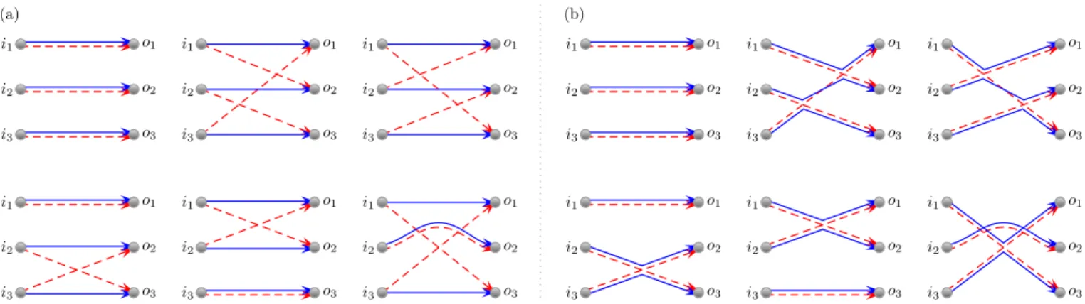
We return first to the transmission probability for bosons in Eq. (9). For a given cycle (1, . . . , l) in the target permutation τ the semiclassical trajectories have a very particular structure whereby we first travel along a trajectory with positive action fromi1 to o1 and then in reverse back along a trajectory with negative action to i2 and so on along a cycle until we return to i1. For example forn= 3 we have the trajectory connections in Fig. 1(a) for each target permutationτ in Eq. (12).
For the actions of the diagram to nearly cancel, and to obtain a semiclassical contribution, the trajectories must be nearly identical, except at small regions called encounters. By directly collapsing the trajectories onto each other, as in Fig. 1(b) we obtain some of the leading order diagrams for each τ. In fact for each diagram, following the rules of [9], the semiclassical contribution is a factor of−N for each encounter and a factor ofN−1 for each link between the encounters. For each cycle of lengthlin the diagrams in Fig. 1(b) one then has a factor of orderN−2l+1.
As a straightforward example we can look at the sim- plest diagrams made up of a set of independent links like the first diagram in Fig. 1(b). Withnlinks each provid- ing the factorN−1 we have the contribution
P˜±=N−n (50)
This contribution is in fact unaffected by the energy and time differences of the incoming particles leading directly to the classical contribution presented in Eq. (7) of the main text. This contribution also accounts for the leading order terms in the expansions of Eqs. (16), (19), (25) and (28).
A. Diagrammatic treatment without time reversal symmetry
Once the contribution of each diagram has been es- tablished, one then needs to generate all permissible di- agrams. As shown in [2, 8] however the vast majority of semiclassical transport diagrams cancel. Those which
remain can be untied until their target permutation be- comes identity. For systems without time reversal sym- metry, which we consider first, they can be mapped to primitive factorisations. One can reverse the process to build the diagrams by starting with a set of nindepen- dent links and tying together two outgoing channels into a new encounter. This tying process increases the or- der of the diagram by N−1. If the outgoing channels are labelled byj andkthen the target permutation also changes toτ(j k). For example going from the top left di- agram of Fig. 1(b) tying together any two outgoing chan- nels leads to the three example along the bottom row.
The diagrams correspondingly move from orderN−3 to N−4.
Tying the remaining outgoing channel to one of those already tied leads to a diagram of the type further along the top row of Fig. 1(b) [for each of which there are 3 possible arrangements, and an alternative with a single larger encounter] and now of orderN−5.
Of course one could retie the same pair chosen in the first step, so that the target permutation is again identity.
Such a diagram is however not shown in Fig. 1(b) but can be thought of as a higher order correction to a diagonal pair of trajectories. These types of diagrams appear when one treats the conductance variance for example. Such diagrams have a graphical interpretation which we will discuss below and use to generate them.
1. Forests
At leading order for each cycle of length l in τ the trajectories however form a ribbon graph in the shape of a tree. The tree has 2l leaves (vertices of degree 1) and all further vertices of even degree greater than 2. Such trees can be generated [10] by first treating unrooted trees whose contributions we store in the generating function f. Using the notation in [7], the function satisfies
f = r N −
∞
X
k=2
f2k−1, f N =
q
1 + 4rN22 −1
2r , (51)
where the power ofrcounts the number of leaves and the encounters may not touch the leads since the channels are distinct. Rooting the tree we add a leave to arrive at the generating functionF =rf while settingr2=swe arrive at
F N =
q1 + N4s2 −1
2 . (52)
Expanding in powers ofs F = s
N − s2 N3 +2s3
N5 −5s4 N7 +14s5
N9 +. . . (53) one has an alternating sequence of Catalan numbers, A000108 [11].
(a) i1
i2
i3
o1
o2
o3
i1
i2
i3
o1
o2
o3
i1
i2
i3
o1
o2
o3
i1
i2
i3
o1
o2
o3
i1
i2
i3
o1
o2
o3
i1
i2
i3
o1
o2
o3
(b) i1
i2
i3
o1
o2
o3
i1
i2
i3
o1
o2
o3
i1
i2
i3
o1
o2
o3
i1
i2
i3
o1
o2
o3
i1
i2
i3
o1
o2
o3
i1
i2
i3
o1
o2
o3
FIG. 1. (a) The permutations on 3 labels represented as trajectory diagrams. (b) Semiclassical contributions come when the trajectories are nearly identical, as when collapsed onto each other.
When summing over all permutations for τ, each cy- cle of length l can be arranged in (l−1)! ways and we now wish to include this factor in the ordinary generating function. First we divide instead by a factor l with the transformation
K0
N = Z F
sN ds= r
1 + 4s
N2 −1 (54)
+1 2ln
N4
1−q 1 + N4s2
2s2 +N2
s
, so thatK0becomes the exponential generating function of the leading order trees multiplied by the factor (l−1)!
as required. To now generate any forest of trees corre- sponding to all permutations τ we can exponentiateK0
to obtain the exponential generating function eK0−1 = s
N +(N−1)s2
2N3 +(N2−3N+ 4)s3 6N5 +(N3−6N2+ 19N−30)s4
24N7 +. . . (55) whose first few terms can be explicitly checked against diagrams.
2. Higher order corrections to trees
For each given cycle (1, . . . , l) of τ there are higher order (in N−1) corrections which can be organised in a diagrammatic expansion [3, 7]. For systems without time reversal symmetry, the first correction occurs two orders lower than leading order and the corresponding diagrams can be generated by grafting the unrooted trees on two particular base diagrams. Repeating the steps in [7], while excluding the possibility for encounters to touch the leads (since the channels are distinct), one first obtains
K2=−(f2+ 3)f4
6(f2+ 1)3 , (56)
where handily, the method for subleading corrections au- tomatically undercounts by a factor of l so we directly obtain the required exponential generating function. Fi- nally we substitute from Eq. (51) and find
12N K2= 1 + N6s2
1 +N4s2
32
−1. (57)
The exponential generating function eK0+K2 −1 would then generate all corresponding diagram sets up to this order.
3. Other corrections
However, the higher order corrections to trees are less important than the higher order corrections to other target permutation structures. For any pair of cycles (1, . . . , k)(k+ 1, . . . , l) inτ we can have diagrams which are orderN−2smaller than a pair of leading order trees.
For example, tying any two outgoing channels of a tree on the cycle (1, . . . , l) would break the target permutation into two as here.
To generate diagrams with two cycles, we graft trees around both sides of a circle as for the cross correlation of transport moments treated in [7]. This will include the example withn = 3 mentioned at the start of this subsection.
Following the steps in [7], while excluding the possibil- ity of encounters touching the lead, one finds the gener- ating function
κ=−ln
1−f12f22 (1−f12)2(1−f22)2
(58) + ln
1 (1−f12)2
+ ln
1 (1−f22)2
,
wheref1andf2are thef in Eq. (51) but with arguments r1andr2respectively. The last two terms are corrections for when eitherr1orr2 is 0 to remove diagrams with no
trees on either side of the circle. In [7], κwas differen- tiated and such terms removed automatically, but here this correction simplifies the result to
κ=−ln
1−f12f22
. (59)
This generating function again undercounts by both a factor ofkand (l−k) and can therefore be thought of as an exponential generating function of both arguments.
Setting s1 = s2 = s then sums the possible splittings of thel elements into two cycles (along with the combi- natorial factor of choosing the label sets), counting each splitting twice. This then provides the following expo- nential generating function
κ1=−1 2ln
1−f4
(60)
=−1 2ln
"
N4 2s2
r 1 + 4s
N2
1 + 2s N2
−1− 4s N2
!#
,
whose expansion is κ1= s2
2N4 −2s3 N6 +29s4
4N8 −26s5
N10 +. . . (61)
4. Order of contributions
With the diagrams treated so far the exponential gen- erating function would be
eK0+κ1+K2−1 = s
N +(N3−N2+N−1)s2 2N5
+(N4−3N3+ 7N2−15N+ 20)s3 6N7
+. . . (62)
and the differences from Eq. (55) occur two orders lower in N−1 than the leading term from independent links.
This is because the additional diagrams required at least two tying operations. However, we wish to know how the contributions change whennscales withN in some way.
First we can compare the contributions coming from K2 to those from K0. In the forest we can replace any tree fromK0with its higher order correction inK2. Since there can be at mostntrees, and the correction is order N−2 smaller, these corrections will be bound by nN−2, up to the scale of the generating function coefficients.
This means that we can expect the contributions from K2 to not be important whenn=o(N2) as we take the limitN→ ∞.
Next we compare the contributions coming fromκ1to those from K0. In the forest we can now replace any tree by breaking its l cycle into two, say k and (l−k).
Alongside the generating function coefficients, the two new cycles come with the factor (l−k−1)!(k−1)! instead
of the (l−1)! that was with the tree. Since 1
(l−1)!
X
k=1
l−1 l
k
(l−k−1)!(k−1)!
=
l−1
X
k=1
l
(l−k)k ≤l , (63)
this contribution is bound by nN−1 and should not be important whenn=o(N).
Continuing in this vein we could break up any tree into three cycles and generate those diagrams but this should also be higher order whenn N. Keeping our expansion to this order we should have
eK0+κ1−1 = s
N +(N2−N+ 1)s2
2N4 (64)
+(N3−3N2+ 7N−12)s3 6N6 +. . .
B. Time reversal symmetry
With time reversal symmetry, additional diagrams be- come possible. For example we may reverse the trajec- tories on one side of the circle used for cross correlations and obtain 2κ1 instead of justκ1. There are also addi- tional base diagrams at the second order correction to trees, which may be treated as in [7], but which we do not treat here since there are now diagrams at the the first order correction. These can be generated by grafting trees around a M¨obius strip. Following again the steps in [7] while excluding the possibility of encounters touching the lead one obtains the generating function
K1= 1 2ln
1−f2 1 +f2
, (65)
or explicitly K1=−1
4ln
1 + 4s N2
(66)
=− s N2 +2s2
N4 −16s2 3N6 +16s4
N8 −256s5 5N10 +. . . Compared to the leading order forest, we could replace any tree by its higher order correction and obtain a term bound bynN−1, again up to the scale of the generating function coefficients. Restricting to n = o(N) the the exponential generating function would be
eK0+2κ1+K1−1 = (N−1)s
N2 +(N2−3N+ 7)s2 2N4 +(N3−6N2+ 28N−75)s3
6N6
+. . . (67)
C. Fermions
For fermions we need to also include the powers of (−1) in Eq. (21). However, because our semiclassical generat- ing functions are organised by cycle type, we simply need to replacesby−sand multiply theK type functions by -1 appropriately.
D. The variance
Now fornbosons we look at
|A˜+n|4= 1 (n!)2
X
P,P0 R,R0∈Sn
n
Y
k=1
Zik,oP(k)Zi∗k,oP0(k)
×Zik,oR(k)Zi∗k,oR0(k), (68) or rather the average
L+n =D
|A˜+n|4E
. (69)
However, when we now compare to Eq. (6) such an av- erage involves summing over permutations of length 2n while each of the originally distinct channels appears ex- actly twice. For example
L+1 =hZi1,o1Zi1,o1Zi∗1,o1Zi∗1,o1i= 2VN(1,1) + 2VN(2), (70) since the delta function conditions in Eq. (6) are satisfied for any choice ofσandπ. The result is
L+1 = 2
N(N+ 1) L+1 = 2
N(N+ 3), (71) without or with time reversal symmetry respectively.
Forn= 2, we can run through the sums of permuta- tions, giving
L+2 = 3N2−N+ 2
N2(N2−1)(N+ 2)(N+ 3), (72) without time reversal symmetry and
L+2 = 3N2+ 5N−16
N(N2−4)(N+ 1)(N+ 3)(N+ 7), (73) with. For largen this process however quickly becomes computationally intractable. Diagrammatically, we can imagine multiplying the sets of diagrams we had before, but also keeping track of all the possible permutations and which channels coincide. For example we could take the diagrams in Fig. 1(b), add the remaining 5 copies of each diagram created by permuting the outgoing labels, and multiply the entire set by itself to obtain pairs of diagrams which appear for the variance. Of course each pair is over counted (n!)2 times and we would still need to account for the diagrams where the pairs interact and
where the repeated channels play a role by considering diagrams acting on 2nleaves.
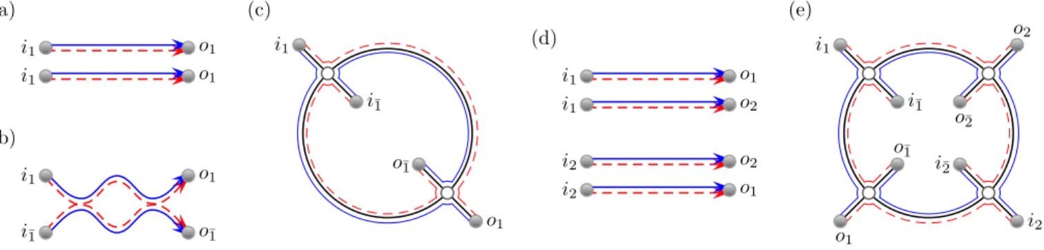
To reduce the difficulty of such a diagrammatic expan- sion, we focus here instead on just calculating the leading order term. We know that these terms are represented di- agrammatically by sets of independent links so we select the (n!)2 such sets from our multiplication. Since each outgoing channel (although appearing twice) is distinct we may relabel them appropriately to reduce our leading order diagrams ton! ways of permuting a single outgoing label. The sum of a product of two permutations essen- tially reduces to a sum over a single permutation. The overcounting is now n! instead. For n = 3 the leading order diagrams are depicted in Fig. 2. For each diagram we have the standard leading order result ofN−2nwhich, when dividing by the over counting, would be the total result if the outgoing channels were different.
However, for each cycle of the effective permutation of the outgoing channels, an additional semiclassical di- agram is possible. By adding a 2-encounter to each pair of identical channels we can separate them into two ar- tificially distinct channels. The resulting semiclassical diagram can be drawn as a series of 2-encounters around a circle with one link on either side. This process is de- picted in Fig. 3. The resulting starting point is from the larger set of possible trajectory correlators than just the sets of independent links squared, but once we move all the encounters into the appropriate leads, the required channels coincide and we have an additional leading or- der diagram.
To count such possibilities we just need to include a power of 2 for each cycle in the permutation of the out- going channels when we include the standard diagonal terms. For each cycle of lengthlthere are (l−1)! differ- ent permutations so that
−2 log(1−s) = 2s+s2+2s3 3 +s4
2 +. . . (74) acts as the exponential generating function of both pos- sibilities for each cycle times their number of permuta- tions. To generate all leading order diagrams we simply exponentiate this function
e−2 log(1−s)−1 = 1
(1−s)2 −1 (75) Since we are still overcounting byn! this actually provides the ordinary generating function and when we include the semiclassical contributions ofN−2n we get the final leading order result of
L+n =n+ 1
N2n +o(N−2n+1) (76) or a variance of
L+n − P˜n+
2
= n
N2n +o(N−2n+1) (77) We checked this against the explicit semiclassical or RMT results involving Eq. (6) forn up to 5. Since the semi- classical diagrams all involve pairs of equally long cycles, the leading order result is also the same for fermions.
(1)(2)(3) i1
i2
i3
o1
o2
o3
i1
i2
i3
o1
o2
o3
(12)(3) i1
i2
i3
o1
o2
o3
i1
i2
i3
o2
o1
o3
(1)(23) i1
i2
i3
o1
o2
o3
i1
i2
i3
o1
o3
o2
(13)(2) i1
i2
i3
o1
o2
o3
i1
i2
i3
o3
o2
o1
(123) i1
i2
i3
o1
o2
o3
i1
i2
i3
o2
o3
o1
(132) i1
i2
i3
o1
o2
o3
i1
i2
i3
o3
o1
o2
FIG. 2. The leading order diagrams for the variance with 3 particles are created by finding semiclassical diagrams with 6 incoming and outgoing channels. When the channels coincide, the leading order diagrams must reduce to separated links corresponding to one of the permutations on 3 labels depicted.
(a)
i1 o1
i1 o1
(b)
i1 o1
i¯1 o¯1
(c) i1
o1
i¯1
o¯1
(d)
i1 o1
i1 o2
i2 o2
i2 o1
(e) i1
o1 i2
o2
i¯1
o¯1
i¯2
o¯2
FIG. 3. (a) A pair of independent links can be joined by an encounter at each end to create the diagram in (b) with artificially distinct incoming and outgoing channels. When the encounters are moved into the incoming and outgoing leads respectively, the channels again coincide leading to a new leading order semiclassical diagram. In the graphical representation, the trajectories in (b) become the boundary walks around both sides of the circle in (c). Starting with four links corresponding to the permutation (12) in (d) we can create the correlated quadruplet represented in (e). Again moving the encounters into the leads creates a new leading order contribution.
Intriguingly, the numerator of the leading order result for the second moments in Eq. (76) is identical to the sec- ond moment of the modulus squared of the permanents ofn×nrandom complex Gaussian matrices [12]. Higher moments of such permanents would be useful to deter- mine the validity of the Permanent Anti-Concentration Conjecture important for Boson Sampling [12]. This opens the possibility that a semiclassical or RMT treat- ment of the higher moments of many body scattering, expanded just to leading order, could help answer such questions.
IV. RELEVANCE OF DIAGRAMS WITH PAIRWISE CORRELATIONS IN THE SCALING
LIMIT
In the following sections we rigurously shown that in the limitn→ ∞and under the scalingN =αn2the sum of semiclassical diagrams with pairwise correlations gives Eq. (15) of the main text ifτd/τs= 0, zij = 0. Once this result is stablished, we re-introduce τd/τs > 0, zij 6= 0 and obtain Eq. (16), one of our main results.
A. The caseτd/τs= 0, zij= 0
In order to show that only diagrams with pairwise cor- relations are neccesary to obtain Eq. (15) in the main text, we start with the following exact relation
hPa,b()i hPa,b(cl)i
τd τs=0
zij=0
= ∂n
∂sn eK0(s)
s=0 (78) expressing the ratio between quantum and classical tran- sition probabilities in terms of the generating function K0(s) defined in Eq. (54). In the limit n, N → ∞ with quadratic scaling N = αn2, all bounds in Sec. III A 4 show we only need to consider standard trees and forests.
The generating function K0 generates trees, with each power ofs corresponding to trees with increasing num- ber of leaves. Justs by itself is individual links, s2 are the pairwise correlations,s3 would be all three way cor- relator and so on. If we truncate to second order we only have links and x-like correlations in our generating func- tion while further exponentiatingK0truncated to second order generates all possible sets of links and pairwise cor- relators, like (a), (b), and (e) but not (d) in Fig. 2 of the main text.
Our strategy is to show that, in the scaling limit, Eq. (78) gives Eq. (15) of the main text when K0 =
s−s2/2N+O(s3) is truncated to second order and there- fore only pairwise correlations are included. Our starting point is then Eq. (78) withK0=s(1−s/2N),
hPa,b()i hPa,b(cl)i
τd τs=0
zij=0
' ∂n
∂sn es(1−2Ns )
s=0, (79) which can be written in the convenient form for asymp- totic analysis
∂n
∂sn es(1−2Ns )
s=0= n!
2πi
I ez(1−2Nz )
zn+1 (80)
= n!
2πi I
ez(1−2Nz )−(n+1) logz as a complex integral along a contour that enlcoses the origin. In the largenlimit this integral can be evaluated in saddle point approximation. The saddle point z=zc is easily found to be
zc= N 2 1−
r
1−4(n+ 1) N
!
'n+1+(n+ 1)2 N . (81) The exponent in Eq. (80) and its second derivative eval- uated at the saddle point are also easily found to be
z 1− z
2N
−(n+ 1) logz
z=zc' −(n+ 1) log(n+ 1) +(n+ 1)−(n+ 1)2
2N , (82)
∂2
∂z2 z
1− z 2N
−(n+ 1) logz z=zc
' 1 n+ 1 to get
∂n
∂sn es(1−2Ns )
s=0' n!
2π
p2π(n+ 1)
((n+ 1)/e)n+1e−(n+1)22N (83) and finally, using the asymptotic approximation for the factorial of large numbers,
∂n
∂sn es(1−2Ns )
s=0'e−2Nn2. (84) We conclude then that in the limitn→ ∞and under the scaling N =αn2 the sum of semiclassical diagrams with pairwise correlations gives Eq. (15) of the main text.
B. The caseτd/τs>0, zij6= 0
If only pairwise correlations are included in the dia- gramatic expansion, all results are expressed in terms of the overlapping functions between all posible pairs of in- coming channels. This is a simple combinatorial problem and we get (forη >1)
hPa,b()i hPa,b(cl)i
−−−−−→n1 N=αnη
X
I⊆{1,...,n}
|I|=:2leven
(−)l Nl
X
CuI l
Y
q=1
Q(2)(zCq), (85)
where C runs over the set of contractions obtained by pairing different indexes inI={i1, . . . , i2l}andCq is its qth element.
C. Mesoscopic HOM effect with two macroscopically occupied channels
In the following the explicit evaluation of Eq. (85) in the case of a very large number n 1 of particles that macroscopically occupy only two different incoming wavepackets is carried out. Let n0 = y0n denote the number of particles in a single incoming wavepacket for which we setz = 0 and letn1 =y1nbe the number of remaining particles occupying a wavepacket with separa- tionz=z1from the other. We denote the corresponding sets of indexes withI0 andI1, respectively.
Pairings of then particle indices are characterized by the total number of pairs l. Furthermore this number splits into the numberl1 of pairs among the n0 indexes in I0, the number k of pairs connecting an index inI0 with one inI1 and the numberl−l1−k of pairs inside I1. Each contraction specified by the numbers l, l1, k contributes a value of
− N
l
[Q(2)(0)]l−k[Q(2)(z1)]k =:
− α
l
n−2lql−k0 q1k (86) to the sum in Eq. (85) if the scalingN=αn2is taken into account. We introduced the abbreviationsq0 andq1 for the two overlap integrals involved. Therefore the prob- ability to get all particles in different outgoing channels is
hPa,b()i hPa,b(cl)i
−−−−−→n1 N=αn2
[n2] X
l=0
min{l,[n21]}
X
l1=0
min{l−l1,n1−2l1}
X
k=0
×Cl,l1,k
− α
l
n−2lql−k0 q1k,
(87)
where the combinatorial factor for each tuple (l, l1, k) is given by
Cl,l1,k= n1
2l1
(2l1−1)!!
| {z } l1 pairs inI1
n1−2l1
k
n0
k
k!
| {z } k pairs betweenI0 andI1
×
n0−k 2l−2l1−2k
(2l−2l1−2k−1)!!
| {z }
remaining pairs inI0
= 1
2l−kl1!(l−l1)!
l−l1
k
×
n1! (n1−2l1−k)!
n0!
(n0−2l+ 2l1+k)!
| {z }
−−−→n1 n2l11+kn2l−2l0 1−k
.
(88)
The limiting value of the expression in square brackets is valid for any fixedl, l1andk. After expressingn0andn1
by their (finite) fractions ofnthe addends of (87) become independent ofn (due to the scalingN =αn2). This is the point where it becomes evident that a scaling of N with a power of n different from η = 2 would lead to trivial results corresponding to Eq. (15) of the main text (for η > 1) also in the present case where τd 6= 0 and zij 6= 0 for somei, j. Simplifying the upper limits of the sums forn→ ∞yields
hPa,b()i hPa,b(cl)i
−−−−−→n1 N=αn2
∞
X
l=0 l
X
l1=0
1 l!
− 2α
l l l1
q0y12l1
y0l−l1
×
l−l1
X
k=0
l−l1
k
(q0y0)l−l1−k(2q1y1)k
=
∞
X
l=0
1 l!
− 2α
l l
X
l1=0
l l1
q0y12l1
2q1y0y1+q0y20l−l1
=
∞
X
l=0
1 l!
− 2α
l
q0 y02+y12
+ 2q1y0y1l
= exph
− 4α
Q(2)(0) 1 +x2
+Q(2)(z1) 1−x2i , (89) where in the last step we rewroteq0 and q1 in terms of overlap functions and introduced the imbalance parame- terxrelated toy0and y1 by
y0=1
2(1−x), y1=1
2(1 +x).
(90)
Equation (89) is plotted and analysed in Fig. 1 of the main text and corresponds to the result Eq. (16) there.
[1] P. W. Brouwer and C. W. J. Beenakker,J. Math. Phys.
37, 4904- (1996).
[2] G. Berkolaiko and J. Kuipers,J. Math. Phys.54, 112103 (2013).
[3] G. Berkolaiko and J. Kuipers,J. Math. Phys.54, 123505 (2013).
[4] J. Novak,E. J. Comb.14, R21 (2007).
[5] S. Matsumoto, Rand. Mat.: Theory Appl. 1, 1250005 (2012).
[6] S. Matsumoto, Rand. Mat.: Theory Appl. 2, 1350001 (2013).
[7] G. Berkolaiko and J. Kuipers,New J. Phys.13, 063020
(2011).
[8] G. Berkolaiko and J. Kuipers, Phys. Rev. E85, 045201 (2012).
[9] S. M¨uller, S. Heusler, P. Braun, and F. Haake, New J.
Phys.9, 12 (2007).
[10] G. Berkolaiko, J. M. Harrison, and M. Novaes,J. Phys.
A41, 365102 (2008).
[11] N. J. A. Sloane, The on-line encyclopedia of integer sequences, published electronically at http://www.research.att.com/∼njas/sequences/
[12] S. Aaronson and A. Arkhipov, Theory Comp. 9, 143- (2013).