Marine emissions of the climate relevant sulfur gases carbonyl sulfide, carbon
disulfide and dimethyl sulfide
Dissertation
zur Erlangung des Doktorgrads
der Mathematisch-Naturwissenschaftlichen Fakultät der Christian-Albrechts Universität zu Kiel
vorgelegt von
Sinikka T. Lennartz
Marine emissions of the climate relevant sulfur gases carbonyl sulfide, carbon
disulfide and dimethyl sulfide
Dissertation
zur Erlangung des Doktorgrads
der Mathematisch-Naturwissenschaftlichen Fakultät der Christian-Albrechts Universität zu Kiel
vorgelegt von
Sinikka T. Lennartz
Kiel, 2017
Referentin: Prof. Dr. Christa A. Marandino Koreferent: Prof. Dr. Hermann W. Bange Tag der mündlichen Prüfung: 28.07.2017
Hiermit erkläre ich,
Sinikka T. Lennartz,
dass ich diese Doktorarbeit selbstständig verfasst sowie alle wörtlichen und inhaltlichen Zitate als solche gekennzeichnet habe.
Die Arbeit wurde unter Einhaltung der Regeln guter wissen- schaftlicher Praxis der Deutschen Forschungsgemeinschaft verfasst.
Sie hat weder ganz noch in Teilen einer anderen Stelle im Rahmen eines Prüfungsverfahrens vorgelegen.
Abstract
Sulfur containing trace gases have gained attention due to their impact on the Earth’s radiative budget and, thus, the climate on our planet. The ocean is a major natural source of the gases carbonyl sulfide (OCS), carbon disulfide (CS2) and dimethyl sulfide (DMS).
Understanding and quantifying their oceanic emissions is critical to decipher their present and future contribution to aerosol formation in the stratosphere (OCS) and troposphere (DMS, CS2). These aerosols exert a natural cooling effect on surface temperatures and therefore counteract global warming. In addition, a well known atmospheric budget of OCS helps to constrain processes in the carbon cycle, in particular the terrestrial CO2 uptake (gross primary production). This is needed to assess the response of the terrestrial biosphere to changing climate conditions. Both, climate predictions and constraining the carbon cycle using OCS, require well quantified sources and sinks of these gases in the atmosphere. However, especially the marine emissions are still associated with considerable uncertainties. A large gap in the atmospheric budget of OCS currently impedes conclusions about trends in stratospheric aerosol formation or gross primary production on a global level. Tropical oceanic emissions of OCS and its precursor gas CS2, potentially also DMS, have been suggested to account for the missing source. In this thesis, newly developed measurement systems as well as numerical models were used in three studies to quantify marine emissions of OCS, CS2 and DMS on local, regional and global scale in order to reduce existing uncertainties.
In the first study, the optimal representation of oceanic emissions in atmospheric models was systematically assessed. Atmospheric chemistry climate models provided with accurate boundary conditions are powerful tools to assess present and predict future climate. Such boundary conditions include emissions of gases from the ocean. The optimal method to represent these emissions in global atmospheric chemistry climate models was investigated by comparing a set-up with prescribed water concentrations and online calculation of emissions to a prescribed static flux climatology. The results indicated that simulated atmospheric mixing ratios agreed best with observations if emissions were calculated
were less sensitive towards online calculation of emissions.
While global DMS surface concentration maps are available in monthly resolution, oceanic measurements of OCS and CS2are still very scarce. Therefore, measuring and modeling sea surface concentrations of OCS, the latter both regionally in the tropics and globally, was the goal of the second study. A novel underway measurement system was developed to measure the trace gas OCS continuously and autonomously during two research cruises. The study areas focused on tropical regions with respect to the missing source of atmospheric OCS. Two contrasting regions, an oligotrophic region in the Indian Ocean as well as the highly productive eastern tropical South Pacific, were chosen to obtain a wide range of concentration variability. The new observations from the tropical regions were used in conjunction with existing data to derive a parameterization for marine photoproduction of OCS, which, for the first time, combines data from three major ocean basins. The parameterization was used to simulate global sea surface concentrations for OCS and derive a global emission estimate of 130 (±80) Gg S yr−1. Results prove the dominant role of marine emissions in the atmospheric budget of OCS, which are nonetheless too low to account for the missing source. Emission estimates of the two other precursor gases complemented the inventory. Despite larger uncertainties in their contributions to the OCS budget, they are also unlikely to fill the gap in the atmospheric budget of OCS.
Characterizing the marine biogeochemical cycling of CS2and OCS in the water column to reduce these uncertainties was subject of the third study. For the first time, both gases were simultaneously measured in the water column of the highly productive eastern tropical South Pacific. A newly developed 1D water column model within the modeling framework GOTM/FABM was used to systematically assess their marine cycling. Model simulations for OCS agreed well with measurements in and below the mixed layer. Additionally, a new parameterization for OCS light-independent production was derived, which confirmed a temperature dependency stable across different biogeochemical regimes. Simulations for CS2profiles provided first field evidence for a significant subsurface degradation pro- cess. A stable ratio in the apparent quantum yield between OCS and CS2across different biogeochemical regimes is promising for future modeling studies.
In total, the results of this thesis improve the understanding of marine emissions of climate relevant sulfur gases and, thus, reduce uncertainties in their atmospheric budget.
The outcome sets the base for future model implementations in order to assess global questions concerning the Earth’s climate.
Zusammenfassung
Schwefelhaltige Spurengase haben durch ihren starken Einfluss auf das Strahlungsbudget der Erde, und damit auf das Klima unseres Planeten, große Aufmerksamkeit erlangt. Der Ozean ist eine bedeutende Quelle der Spurengase Karbonylsulfid (OCS), Kohlenstoffdisulfid (CS2) und Dimethylsulfid (DMS). Das Verständnis und die Quantifizierung dieser Emissio- nen aus dem Ozean sind wichtig, da sie zur Aerosolbildung in der Stratosphäre (OCS) und Troposphäre (DMS, CS2) beitragen. Sie üben daher einen natürlichen Kühlungseffekt auf die Oberflächentemperatur der Erde aus, welcher der globalen Erwärmung entgegenwirkt.
Zusätzlich kann über das atmosphärische OCS-Budget die nicht direkt messbare pflan- zliche CO2Aufnahme (Bruttoprimärproduktion) indirekt abgeleitet werden. Ein besseres Verständnis der Bruttoprimärproduktion ist notwendig, um die Reaktion der terrestrischen Biosphäre auf wechselnde Klimabedingungen abzuschätzen. Daher sind exakt quantifizierte Quellen und Senken von OCS, CS2und DMS notwendig, da letztere in der Atmosphäre zu OCS reagieren können. Eine große Lücke im atmosphärischen Budget von OCS erschwert momentan Rückschlüsse auf die Bildung von stratosphärischen Aerosolen, sowie auf die Bruttoprimärproduktion auf globaler Ebene. In diesem Zusammenhang haben die ozeani- schen Emissionen von OCS und seinen Ausgangsstoffen an Aufmerksamkeit gewonnen, da Emissionen aus tropischen Ozeanregionen als fehlende Quelle angenommen werden.
In der vorliegenden Dissertation wurden neu entwickelte Messsysteme sowie numerische Modelle in drei Studien eingesetzt, um die marinen Emissionen der Spurengase OCS, CS2 und DMS lokal, regional und global zu quantifizieren.
In der ersten Studie wurde systematisch ausgewertet, wie Ozeanemissionen optimal in at- mosphärische Klimamodelle eingebunden werden können. Diese sind wichtige Werkzeuge für die Erforschung des gegenwärtigen Klimas und die Vorhersage zukünftiger Trends, sofern sie mit sinnvollen Rahmenbedingungen ausgestattet werden. Solche Rahmenbe- dingungen sind unter anderem die Ozeanemissionen von Spurengasen. In dieser Studie wurden Modellläufe mit vorgeschriebenen Wasserkonzentrationen und einer interaktiven Berechnung der Emissionen mit Modellläufen mit statisch vorgeschriebenen Emissionskli-
der Simulation interaktiv berechnet werden. Das gilt insbesondere für Gase, die im Ozean nahe am Lösungsgleichgewicht konzentriert sind. Gase, deren Wasserkonzentrationen weiter vom Lösungsgleichgewicht entfernt sind, waren weniger sensitiv gegenüber der interaktiven Emissionsberechnung.
Während für DMS globale Ozeankonzentrationen in monatlicher Auflösung vorliegen, sind für OCS und CS2relativ wenig Messdaten vorhanden. Deshalb war das Ziel der zweiten Studie, OCS im Oberflächenwasser des tropischen Ozeans zu messen, sowie dessen Ober- flächenkonzentrationen auf regionaler und globaler Ebene zu simulieren. Dazu wurde ein neues Messsystem entwickelt, mit dem OCS kontinuierlich und automatisiert während zwei Forschungsfahrten gemessen wurde. Vor dem Hintergrund der fehlenden atmosphärischen Quelle von OCS wurde der Fokus auf tropische Regionen gelegt, da hier die Datenlage bisher unzureichend war. Zwei sehr unterschiedliche tropische Gebiete – eine oligotrophe Region im Indischen Ozean sowie eine hochproduktive Region im östlichen Südpazifik – wurden ausgewählt, um einen großen Bereich der Variabilität der Oberflächenkonzen- trationen abzudecken. Mit den neu erhaltenen Daten wurde eine neue Parametrisierung für die marine Photoproduktion von OCS aufgestellt, die erstmalig Informationen aus allen drei großen Ozeanen kombiniert. Diese Parametrisierung wurde zur Berechnung glo- baler Oberflächenkonzentrationen von OCS verwendet. Die Abschätzung direkter globaler Emissionen beläuft sich auf 130±80 Gg S a−1. Die Ergebnisse belegen die wichtige Rolle ozeanischer Emissionen, sind jedoch zu niedrig, um die Lücke im atmosphärischen Budget von OCS zu schließen. Auch indirekte OCS-Emissionen durch die Ausgangsstoffe CS2und DMS können die Lücke wahrscheinlich nicht schließen.
Die Charakterisierung mariner Stoffkreisläufe von OCS und CS2waren daher Gegenstand der dritten Studie. Erstmalig wurden Konzentrationsprofile beider Gase in der Wassersäule im biologisch hochproduktiven tropischen Südostpazifik gemessen. Ein neu entwick- eltes 1D-Wassersäulenmodell in der Modellumgebung GOTM/FABM wurde verwendet, um die biogeochemischen Prozesse beider Gase systematisch zu untersuchen. Mit dem neu entwickelten Modell konnten die Messungen von OCS in der Wassersäule sehr gut reproduziert werden. Zusätzlich wurde eine neue Parametrisierung für die lichtunab- hängige OCS-Produktion entwickelt. Simulationen der CS2-Profile geben Hinweise auf einen Abbauprozess unterhalb der Mischungsschicht, für den bisher kein Reaktionsprozess bekannt ist. Der für die Bestimmung der Photoproduktionsrate wichtigeapparent quantum yieldbeider Gase zeigte über verschiedene biogeochemische Regionen hinweg ein stabiles Verhältnis, was vielversprechend für zukünftige kombinierte Modellstudien ist.
Die Ergebnisse liefern eine Grundlage für weitere Modellimplementierungen, um globale Fragen bezüglich des Klimas der Erde zu beantworten.
Manuscript contributions
This dissertation is based on the following manuscripts:
1. Lennartz, S. T., Krysztofiak, G., Marandino, C. A., Sinnhuber, B. M., Tegtmeier, S., Ziska, F., Hossaini, R., Krüger, K., Montzka, S. A., Atlas, E., Oram, D. E., Keber, T., Bönisch, H., and Quack, B.: Modelling marine emissions and atmospheric dis- tributions of halocarbons and dimethyl sulfide: The influence of prescribed water concentration vs. Prescribed emissions, published in: Atmos. Chem.
Phys., 15, 11753-11772, 10.5194/acp-15-11753-2015, 2015.
My contribution: I designed the study together with GK, CAM, BMS, BQ and KK, performed the simulations together with GK, analysed the data together with GK, and wrote the manuscript with contributions from all authors.
2. Lennartz, S. T., Marandino, C. A., von Hobe, M., Cortes, P., Quack, B., Simo, R., Booge, D., Pozzer, A., Steinhoff, T., Arevalo-Martinez, D. L., Kloss, C., Bracher, A., Röttgers, R., Atlas, E., and Krüger, K.: Direct oceanic emissions unlikely to ac- count for the missing source of atmospheric carbonyl sulfide, published in:
Atmos. Chem. Phys., 17, 385-402, 10.5194/acp-17-385-2017, 2017.
My contribution: I designed the study with CAM and MvH, developed the measure- ment system, performed shipboard measurements and OCS model studies, and wrote manuscript with contributions from all authors.
3. Lennartz, S.T., Marandino, C.A., von Hobe, M., Fischer, T., Bittig, H., Booge, D., Goncalves-Araujo, R., Ksionzek, K., Koch, B.P., Bracher, A., Röttgers, R., Quack, B.: Production and Consumption processes of OCS and CS2in the Eastern Tropical South Pacific, manuscript in preparation for JGR.
My contribution: I designed the study together with CAM, performed shipboard measurements and sampling, developed the GOTM/FABM module together with HB, and wrote the manuscript with contributions from all authors.
1. Campbell, E., Kesselmeier, J., Yakir, D., Berry, J. A., Peylin, P., Belviso, S., Vesala, T., Maseyk, K., Seibt, U., Chen, H., Whelan, M., Hilton, T., Montzka, S.,Lennartz, S.T., Kuai, L., Wohlfahrt, G., Wang, Y., Blake, N., and Blake, D.: Assessing a new clue to how much carbon plants store, EOS Earth and Space Science News, 2017,in press.
2. Schlundt, C., Marandino, C. A., Tegtmeier, S.,Lennartz, S. T., Bracher, A., Cheah, W., Krüger, K., and Quack, B.: Oxygenated volatile organic carbon in the western pacific convective centre: Ocean cycling, air-sea gas exchange and atmospheric transport, Atmos. Chem. Phys. Discuss., 2017, 1-29, 10.5194/acp-2017-9, 2017.
3. Falk, S., Sinnhuber, B. M., Krysztofiak, G., Jöckel, P., Graf, P., andLennartz, S. T.: Brominated VSLS and their influence on ozone under a changing climate, Atmos.
Chem. Phys. Discuss., 2017, 1-24, 10.5194/acp-2017-34, 2017.
4. Whelan, M. and COSANOVA Team: Synthesis on Carbonyl Sulfide as a tracer for terrestrial gross primary production. Manuscript, 2017.
Acknowledgments
First and foremost, I would like to thank Prof. Dr. Christa Marandino for supervising my thesis, for sharing her contagious enthusiasm for science, and for keeping the perfect balance between guidance and freedom to let me pursue my own scientific ideas. I am very grateful to Dr. Birgit Quack for her commitment, for her thorough feedback throughout my thesis and for asking the right questions at the right time. Furthermore, I highly appreciated the assistance of Dr. Marc von Hobe, who not only trusted me in deploying his precious OCS analyzer on ships in the middle of the ocean, but also for sharing his great knowledge and experience in measuring and modeling OCS. I also would like to thank the members of my ISOS-committee, Christa, Birgit, Dr. Irene Stemmler and Prof. Dr. Andreas Oschlies, for their valuable input during discussions in my semiannual committee meetings, which always provided me with a new perspective.
The members of the Marine Chemistry Department have immensely contributed to making my time as a PhD student productive and enjoyable. A huge ’Thank you!’ to Alex and Dennis (the Golden T.C. Racing Team I), who hold a major share in making my PhD time unforgettable. Especially for you: Thank you for the music! A special ’Thank you!’ to the current and former members of the HPA (and beyond), who were always open for questions, moral support and Friday afternoon beer: Alina, Anna, Annette, Cathleen, Damian, Helmke, Jimmy, Katharina, Kathrin, Meike, Melf, Roberto, Steffen, Tobi (x2). I am very grateful for the friendships that developed during this time. Also, I highly acknowledge the support of Damian and Tobi, for their technical help during two cruises in solving seemingly impossible-to-solve problems with their experience and inexhaustible pool of emergency lab material. Tim is thanked for his incredible patience in making physical oceanography understandable to me. Thanks to Nils for valuable IT support in exchange for burgers. I would also like to thank the TLZ, namely Wiebke, René, Rudi, and Uwe, for transforming my crazy ideas into deployable systems.
I acknowledge funding of my research from the BMBF (ROMIC-THREAT) and Prof. Dr.
Christa Marandino’s Helmholtz Young Investigators Group TRASE-EC.
Contents
1 Introduction 1
1.1 Sulfur and its role in climate . . . 1
1.1.1 Carbonyl Sulfide (OCS) . . . 5
1.1.2 Carbon disulfide (CS2) . . . 9
1.1.3 Dimethyl sulfide (DMS) . . . 10
1.2 Air-sea gas exchange . . . 12
1.3 Marine biogeochemistry of volatile organic sulfur compounds . . . 14
1.3.1 Carbonyl sulfide (OCS) . . . 15
1.3.2 Carbon disulfide (CS2) . . . 17
1.3.3 Dimethyl sulfide (DMS) . . . 18
1.4 Objectives and Research Questions . . . 19
2 Methods 33
2.1 In-situ measurements of OCS and CS2 . . . 332.1.1 A new underway measurement system for OCS . . . 33
2.1.2 A profiling pump for continuous depth profiles of OCS . . . 37
2.1.3 Measurements of CS2with GC-MS . . . 38
2.2 A new database for marine measurements of OCS and CS2 . . . 40
2.3 Box and 1D models for OCS and CS2 . . . 42
2.3.1 Parameterizations for OCS . . . 42
2.3.2 Parameterizations for CS2 . . . 45
2.3.3 A simple box model to simulate sea surface concentrations . . . 46
2.3.4 1D water column models for OCS and CS2 . . . 48
2.4 The global atmospheric 3D chemistry climate model EMAC . . . 49
3 Modelling marine emissions 55
3.1 Introduction . . . 57
3.2 Model set-up and data description . . . 59
3.2.1 The atmosphere-chemistry model EMAC . . . 59
3.2.2 Parameterizations of air-sea gas exchange . . . 60
3.2.3 Experimental Set-up . . . 62
3.2.4 Observational data . . . 66
3.3 Results and Discussion . . . 69
3.3.1 Global emissions based on prescribed concentrations . . . 69
3.3.2 Atmospheric mixing ratios based on PWC and PE . . . 73
3.3.3 Comparison of different transfer velocity (kw) parameterizations . 81 3.4 Summary and conclusions . . . 82
3.5 Acknowledgments . . . 83
3.6 Appendix: Supplementary figures . . . 84
3.7 Appendix: Supplementary tables . . . 86
3.8 Appendix: Equations to compute error metrics . . . 88
4 Direct oceanic emissions of OCS 99
4.1 Introduction . . . 1004.2 Methods . . . 104
4.2.1 Study sites . . . 104
4.2.2 Measurement setup for trace gases . . . 104
4.2.3 Calculation of air–sea exchange . . . 106
4.2.4 Box model of OCS concentration in the surface ocean . . . 107
4.2.5 Assessing the indirect contribution of DMS with EMAC . . . 110
4.3 Results and discussion . . . 111
4.3.1 Observations of OCS in the tropical ocean . . . 111
4.3.2 A direct global oceanic emission estimate for OCS . . . 114
4.3.3 Indirect OCS emissions by DMS and CS2 . . . 120
4.4 Conclusions and outlook . . . 121
4.5 Data availability . . . 123
4.6 List of parameters . . . 123
4.7 Acknowledgements . . . 123
4.8 Appendix: Supplementary figures . . . 125
4.9 Appendix: Supplementary tables . . . 130
5 OCS and CS
2production and loss processes in
the eastern tropical South Pacific 141
5.1 Introduction . . . 142
5.2 Methods . . . 145
5.2.1 Study area . . . 145
5.2.2 Measurements of trace gases . . . 145
5.2.3 Measurements of ancillary parameters . . . 147
5.2.4 Modeling OCS and CS2concentration in the water column . . . 149
5.3 Results . . . 153
5.3.1 Characterization of dissolved organic matter . . . 153
5.3.2 Carbonyl sulfide (OCS) . . . 156
5.3.3 Carbon disulfide (CS2) . . . 159
5.4 Discussion . . . 164
5.4.1 Carbonyl sulfide (OCS) . . . 164
5.4.2 Carbon disulfide (CS2. . . 167
5.5 Summary and conclusion . . . 170
6 Conclusion and Outlook 179
List of Figures
1.1 Global atmospheric sulfur budget in volcanically quiescent periods. . . 2
1.2 Radiative forcing and aggregated uncertainties from 2011 in relation to 1750. 4 1.3 Uncertainties in the atmospheric budget of carbonyl sulfide. . . 6
1.4 Conceptual model of air sea exchange and uncertainties in the transfer velocityk . . . 13
1.5 Research questions addressed in this thesis. . . 20
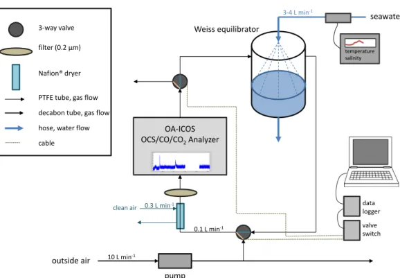
2.1 Set-up for continuous OCS measurements at sea. . . 35
2.2 Comparison of the effect of the inlet gas stream on the OCS mixing ratio at the outlet of the membrane equilibrator. . . 37
2.3 Set-up of profiling pump for water column measurements of OCS. . . 38
2.4 Specifications for CS2measurements with GC-MS. . . 40
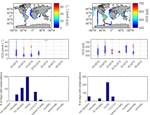
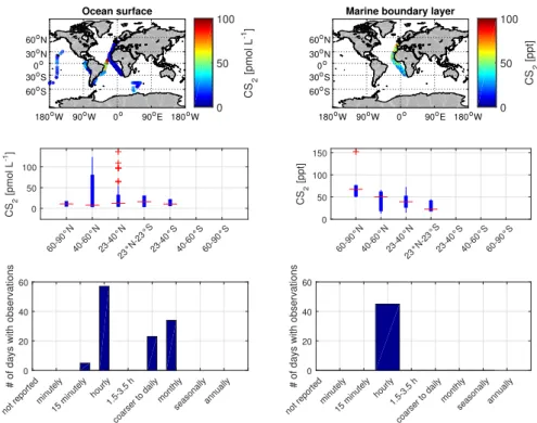
2.5 Metadata of OCS in the newly developed database . . . 41
2.6 Metadata of CS2in the newly developed database . . . 42
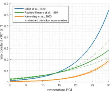
2.7 Hydrolysis rates for OCS from previous experimental studies. . . 44
2.8 Set-up of the simple mixed layer box model for carbonyl sulfide (OCS). . . 47
2.9 Model set-up for the 1D water column models for OCS and CS2. . . 49
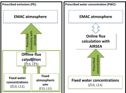
3.1 Schematic overview of the set-up of prescribed emissions and online cal- culated fluxes based on prescribed water concentrations implemented in EMAC. . . 63
3.3 Locations of atmospheric data of aircraft and ship campaigns for halocar- bons and DMS for comparison with EMAC model output. . . 68
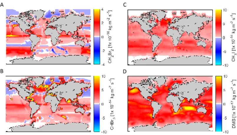
3.4 Emissions from prescribed water concentrations for halocarbons and DMS in EMAC. . . 70
3.5 Differences in emissions of halocarbons and DMS between prescribed emis- sions and water concentrations in EMAC . . . 72
3.6 Atmospheric mixing ratios from EMAC model output and observations for 3 halocarbons. . . 74 3.7 Mean seasonal variation of CH2Br2mixing ratios. . . 76 3.8 Mean seasonal variation of CHBr3mixing ratios. . . 77 3.9 Mean seasonal variation of CH3I mixing ratios. . . 78 3.10 Mean seasonal variation of DMS mixing ratios. . . 79 3.11 Taylor diagram of PE compared to PWC for DMS and three halocarbons. . 80 3.12 Numbers of measurement per 10◦latitude bin for Figure 7. . . 84 3.13 Input parameters for case study box model simulation for the ASTRA-OMZ
cruise. . . 85 4.1 Observed OCS water concentrations and calculated emissions during three
cruises to the tropical oceans. . . 113 4.2 OCS box model simulations compared to observations for the cruises OASIS
and ASTRA-OMZ. . . 116 4.3 Dependence of photoproduction rate constantpona350. . . 117 4.4 Annual simulated mean surface concentration of OCS and corresponding
emissions. . . 118 4.5 CS2surface concentrations during two cruises to tropical oceans. . . 120 4.6 Input parameters for case study box model simulation for the OASIS cruise. 125 4.7 Input parameters for case study box model simulation for the ASTRA-OMZ
cruise. . . 126 4.8 Annual mean for input parameters for the global box model simulation. . . 127 4.9 Diurnal cycles of downward radiation as forcing for the global mixed layer
OCS model. . . 128 4.10 Production and consumption rates from global box model simulation. . . . 129 5.1 Sea surface temperature (SST) along the cruise track of ASTRA-OMZ (SO243) 144 5.2 CDOM, absorption spectra slope and SPE-DOS during ASTRA-OMZ (SO243). 154 5.3 FDOM components of PARAFAC analysis in the ETSP . . . 155 5.4 UV-FDOM and VIS-FDOM components along the cruise track of ASTRA-
OMZ (SO243). . . 156 5.5 Concentrations of OCS and CS2along the cruise track of ASTRA-OMZ. . . 157 5.6 Observed, simulated and residual concentration profiles of OCS at the
stations 2, 5, 7 and 18 along the cruise track of ASTRA-OMZ. . . 158 5.7 OCS fluxes within the water column derived from measured concentrations
and microstructure profiles. . . 159
5.8 Daily averaged profiles of production and loss processes of OCS for sta- tions 2, 5, 7, and 18 during the ASTRA-OMZ cruise as simulated with the FABM/GOTM model. . . 160 5.9 Arrhenius-plot of temperature dependency of dark production rates of OCS. 161 5.10 Observed, simulated and residual concentration profiles of CS2the stations
2, 5, 7 and 18 along the cruise track of ASTRA-OMZ. . . 162 5.11 Photoproduction rates of CS2at stations 2, 5, 7, and 18 as simulated with
the FABM/GOTM model. . . 163 5.12 CS2fluxes within the water column as derived from measured concentra-
tions and microstructure profiles. . . 163 6.1 Level of previous knowledge and contribution of this thesis towards compre-
hensively modeling sulfur emissions of OCS, CS2and DMS in 3D numerical models. . . 180 6.2 Annual mean direct and indirect marine emissions of OCS . . . 182 6.3 Seasonality and latitudinal dependence of global direct and indirect marine
OCS emissions. . . 184 6.4 Comparison of spatial patterns in CDOM and DOM . . . 185
List of Tables
3.1 Set-up of EMAC model simulations for comparison of prescribed water concentrations and prescribed emissions. . . 64 3.2 Integrated global emissions for halocarbons and DMS during 2010-2011
(sensitivity tests) . . . 67 3.3 Metadata of the ground based time series (halocarbons, DMS) stations for
comparison of EMAC model output . . . 69 3.4 Integrated global fluxes of halocarbons and DMS from this study compared
to previously available emission inventories. . . 71 3.5 Error metrics of EMAC model output compared to observations for pre-
scribed emissions and prescribed water concentrations of halocarbons and DMS. . . 80 3.6 Global averages of marine emissions for the year 2012 as a comparison for
the resolution of grid T42 and T106. . . 86 3.7 Overview of data of the aircraft campaigns (halocarbons, DMS) used in this
study. . . 87 4.1 OCS missing source estimates derived from top-down approaches. . . 101 4.2 Global oceanic emission estimates of OCS. . . 103 4.3 Descriptive statistics of trace gases and related parameters as observed
during three cruises to tropical oceans . . . 112 4.4 Comparison of water properties. . . 114 4.5 Comparison of previous observations with model output. . . 115 4.6 Input parameters for the box model for the OASIS cruise (Indian Ocean) . 130 4.7 Input parameters for the box model for the ASTRA-OMZ cruise (Pacific
Ocean) . . . 130 4.8 Input parameters for the global box model. . . 131
5.1 Simulation set-up for the GOTM/FABM model simulations at 4 stations for the two gases OCS and CS2. . . 152 5.2 Fitted AQY for stations 2, 5, 7, and 18 with error metrics. . . 167
1
Introduction
1.1 Sulfur and its role in climate
The climate of the Earth critically depends on the interaction between atmosphere, ocean, ice and land masses to absorb and redistribute solar energy. The atmosphere plays a key role in this context, as its composition strongly influences the radiative budget of the Earth.
The concentration of trace gases and aerosols in the atmosphere determines the reflection, absorption and transformation of incoming solar radiation, and thus influences the tem- perature of the planet. Sulfur containing trace gases play an important role in defining the radiative balance of the Earth with both warming and cooling effects. Sulfate aerosols, which form by oxidation of precursor gases such as carbonyl sulfide (OCS) and sulfur dioxide (SO2), reflect solar radiation and thus increase Earth’s albedo in the stratosphere and the troposphere (Boucher et al., 2013; Kremser et al., 2016). Secondary aerosols from biogenic trace gases such as dimethyl sulfide (DMS) might alter the formation and lifetime of clouds with an impact on albedo as well, although still associated with high uncertainty (Andreae & Crutzen, 1997). Besides the cooling effect, some sulfur gases (OCS, CS2) also act as greenhouse gases with a warming effect (Brühl et al., 2012). Describing the radiative budget in our current as well as in future climate scenarios requires both, an accurate process understanding of the mechanisms that alter solar radiation in the atmosphere, as well as an exact quantification of the atmospheric budget, i.e. the sources and sinks, of sulfur containing trace gases. The atmospheric sulfur budget is fed by both natural and anthropogenic sources. Natural biogenic sulfur emissions include a variety of reduced gases (DMS, OCS, CS2, H2S, dimethyl sulfide) from oceanic emissions (Andreae, 1986; Liss et al., 2014), wetlands and soils (Bates et al., 2004)(Fig. 1.1). Emissions from volcanoes and, to a smaller amount, from dust storms, appear less regular and often only for a short time,
e1.1:GlobalbudgetofatmosphericsulfurcompoundsfromShengetal.(2015).Boxesrepresentreservoirs(GgS)andarrowsthedirectionoffluxes(GgSyr−1.Numbersarecolorcodedtoindicateresultsfromdifferentmodelsimulationsorobservations(black:AER-2Dwithsensitivityresultsinparenthesis,measurementsinbracketsfromSPARC(2006),red:SOCOL-AER,green:troposphericGOCARTfromChin&Davis2000,blue:GE-2derivedaerosolmass(Arfeuille2013),orange:Chin&Davis(1995)).
but can introduce substantial amounts of sulfur gases such as SO2up to the stratosphere (Kremser et al., 2016). Besides these natural emissions, the atmospheric sulfur reservoir is strongly affected by human activities (Brimblecombe et al., 1989; Rodhe, 1999). Rodhe (1999) estimated the human emissions of sulfur to the atmosphere to be as large as 2-3 times the magnitude of natural emissions. This is because of emissions of SO2from coal and petroleum burning, and leads to a continuous rise of atmospheric sulfuric acid (H2SO4) since the beginning of the Industrial Revolution, which is even detectable in ice cores (Mayewski et al., 1990). Higher atmospheric concentrations of H2SO4increase the acidity of rainwater with serious negative environmental effects (Likens & Bormann, 1974). The atmospheric sulfur cycle is thus a complex superposition of natural biogenic sulfur emissions, irregular volcanic eruptions and strong human perturbations. In order to understand this complexity, it is crucial to separate the single natural processes from the anthropogenic impact and reduce uncertainties in the fluxes between reservoirs.
High turnover rates make the atmospheric sulfur cycle react quickly to changes in environmental conditions and emissions. This close connection between source fluxes and effects can lead to feedback mechanisms with mitigating or amplifying effects on global warming (Boucher et al., 2013). Aerosol-climate feedbacks including secondary aerosols from biogenic sulfur gas emissions occur through changes in source strength of aerosols or their precursors (Boucher et al., 2013). For example, DMS has been suggested to be involved in a feedback mechanism (Charlson et al., 1987, see section 1.1.3), but the overall effect is currently associated with only a medium level of confidence (Boucher et al., 2013).
Hence, quantifying the source strength of sulfur containing trace gases is important to assess the magnitude of such feedback mechanisms.
Despite the importance of atmospheric sulfur gases, their effects, budgets and fluxes between reservoirs carry high uncertainties. While aerosols provide an important natural counterpart to anthropogenic global warming, their overall effect on the radiative balance of the Earth still displays large uncertainty even in the direction of the impact (Fig. 1.2), resulting among others from uncertainty in effects and source strength of aerosol precursors.
For global atmospheric sulfur budgets, estimated total emission of sulfur ranges between 82.5 Tg S yr−1and 108.3 Tg S yr−1, with resulting differences of approximately 30% (Chin et al., 2000; Sheng et al., 2015). Relative uncertainties in the source strength of single sulfur species are much higher. For example, emissions of OCS and CS2are associated with uncertainties of a factor of 2-4 for OCS (Kremser et al., 2016), and are even less well constrained for CS2. Although the source strength of OCS and CS2on the order of several hundreds of Gg S per year is much smaller than the total atmospheric sulfur source strength in the teragram range, there are specific effects particular to these gases that require their
Figure 1.2:Globally averaged radiative forcing and aggregated uncertainties from 2011 in relation to 1750 (IPCC AR5). Black diamonds are best estimates together with uncertainty range and the level of confidence given at the last column of the table (VH - very high, H - high, M - medium, L - low.
budgets to be well constrained (see section 1.1.1 and 1.1.2). For example, CS2is the most important precursor of OCS, and OCS the major supplier of the stratospheric aerosol layer in volcanically quiescent periods (Kremser et al., 2016). Stratospheric aerosols have increased since 2000 with a small but significant impact on global surface temperatures (Solomon et al., 2011). Neglecting the variations in the global stratospheric aerosol layer can lead to an overestimation of global warming (Solomon et al., 2011). Therefore, accurately quantifying the individual contributions of major suppliers to stratospheric aerosols is important to identify reasons for the temporal variations in the stratospheric aerosol layers.
Understanding the atmospheric sulfur budget and quantifying the fluxes in and out of the atmosphere as well as understanding the driving processes is crucial for assessment and prediction of climate in present and future. The ocean plays a major role as one of the largest sulfur emitters (Liss et al., 2014). Oceanic sulfur emissions represent the largest natural flux of sulfur to the atmosphere (Chin et al., 2000). Sulfur gases emitted by the
ocean are mainly reduced compounds, and include in descending order of the amount of annual emissions, DMSmethyl mercaptane (CH3SH) > OCS, CS2> H2S (Liss et al., 2014). In this thesis, the focus is set on the gases OCS and CS2, as especially the marine contribution of their emissions is associated with uncertainties of up to a factor of four of global annual emissions (see below). DMS is quantitatively the most important compound to transport sulfur from the ocean to the atmosphere, and its emissions are reasonably well quantified based on measurements and model studies (see e.g. Kloster et al., 2006; Lana et al., 2011). This thesis builds upon the previous knowledge by using DMS climatologies to assess how to best represent marine sulfur emissions in stand-alone atmospheric climate models, to provide a tool for dynamically including oceanic sulfur emissions for global climate assessment.
1.1.1 Carbonyl Sulfide (OCS) in the atmosphere
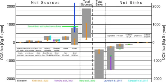
Carbonyl sulfide (OCS) is the most abundant sulfur gas in the atmosphere with an annual mean mixing ratio of approximately 500 ppt (Liss et al., 2014; Sheng et al., 2015). OCS is emitted to the atmosphere from the oceans by both direct and indirect emissions of the precursor gas CS2(and potentially DMS, see below), as well as from biomass burning and other anthropogenic sources. Sinks of atmospheric OCS are dominated by vegetation uptake, and uptake by soils and destruction by the OH radical are smaller but still significant (Chin & Davis, 1993; Kremser et al., 2016; Watts, 2000)(Fig. 1.3).
Spatial and temporal variations of atmospheric OCS mixing ratios occur on several scales.
Although interannual variability on decadal timescales is low, a pronounced seasonal cycle leads to variations of∼100 ppt within one year, with a minimum in late summer and a maximum in spring (Montzka et al., 2007). Variations in atmospheric mixing ratios are stronger on millennial time scales. As inferred from firn ice and ice core measurements dating back ca. 55000 years B.P., atmospheric mixing ratios in Antarctica were as low as 160-210 ppt at the beginning of the Holocene (Aydin et al., 2016). On the spatial scale, several lines of evidence indicate a latitudinal gradient for atmospheric mixing ratios of OCS at least in some locations (Krysztofiak et al., 2015; Kuai et al., 2015). Ground based stations from the NOAA-ESRL (Earth System Research Laboratory) show constant air mixing ratios in the southern hemisphere (3 stations) and the tropics, but a decline in atmospheric volume mixing ratios towards high latitudes in the northern hemisphere, reflecting the uptake of OCS by vegetation in boreal latitudes (Montzka et al., 2007). The atmospheric lifetime of OCS is estimated between 2 and 7 years, which is long enough for mixing in the two hemispheres and to enable entrainment into the stratosphere, where OCS is rapidly photolysed (Kremser et al., 2016).
Figure 1.3:Uncertainties in the atmospheric budget of carbonyl sulfide (Kremser et al., 2016).
A well explained atmospheric budget is required for two reasons: First, OCS is a climate relevant trace gas and accurate fluxes are needed to derive an accurate atmospheric budget to assess its effect on climate. Second, OCS has shown potential as a proxy to constrain terrestrial gross primary production (Berry et al., 2013; Campbell et al., 2008), for which a well defined budget is needed to apply this proxy on the global scale (Beer et al., 2010).
Climate relevance of OCS
OCS is relevant to global climate in several ways with counteracting warming and cooling effects (Brühl et al., 2012). In the troposphere, OCS acts as a greenhouse gas with a direct radiative forcing efficiency 724 times that of CO2(Brühl et al., 2012). However, the much lower atmospheric mixing ratio of OCS (ppt) compared to CO2(ppm) reduces the overall warming effect considerably relative to other greenhouse gases such as CO2. Due to its long lifetime, OCS can be transported to the stratosphere, where it acts as a precursor to stratospheric sulfate aerosols (Crutzen, 1976; Kremser et al., 2016). In volcanically quiescent periods, the upward transport of OCS controls the aerosol loading of the Junge layer in the stratosphere (Brühl et al., 2012). There, OCS is photolysed to SO2which reacts with OH to form H2SO4, yielding sulfate aerosols (Kremser et al., 2016). These sulfate aerosols reflect sunlight and thus increase Earth’s albedo (Junge et al., 1961), therefore resulting in a cooling effect on global temperatures. Brühl et al. (2012) showed that the warming and the cooling effect balance each other on a global scale, but can lead to local differences. The net effect can potentially vary with changes in source strength and location
of emissions as well as atmospheric circulation over time. In contrast, Solomon et al. (2011) showed that model simulations overestimate global warming, if the cooling effect of the stratospheric aerosol layer supplied by OCS is not considered. A better understanding of sources and sinks of tropospheric OCS is needed to improve future climate prediction (Kremser et al., 2016).
Besides the cooling effect, the stratospheric aerosols also influence ozone depletion, as they support the formation of polar stratospheric clouds (Solomon et al., 2015). The ozone content in the polar atmosphere has been shown to be very sensitive to the aerosol loading (Solomon et al., 2015), as these aerosols provide the surfaces for heterogeneous reactions that accelerate ozone depletion. A change in carbonyl sulfide loading, aerosol formation and consequently ozone depletion could have potential feedbacks in the coupled system of ocean and atmosphere.
Currently, atmospheric chemistry climate models often use prescribed mixing ratios of OCS in the boundary layer instead of seasonally varying boundary fluxes (Brühl et al., 2012; Sheng et al., 2015). Simulations would benefit from temporally and spatially resolved boundary fluxes of sulfur containing trace gases to dynamically take into account variations in emissions and sulfur loading of the atmosphere (Kremser et al., 2016). At the moment, such simulations hampered by a poorly constrained atmospheric budget of OCS, in which known sinks exceed known sources of OCS to the atmosphere, so model simulations can not spin up to equilibrium.
Constraining gross primary production with OCS
In addition to its climate relevance, OCS recently regained attention as a CO2 analog to constrain terrestrial gross primary production (GPP, Berry et al., 2013; Campbell et al., 2008). The global application of using OCS as a proxy for GPP was discovered as CO2 and OCS both show a remarkable covariance in their seasonal cycle at ground based time series stations (Montzka et al., 2007) and airborne data (Campbell et al., 2008). Constraining processes in the biological part of the carbon cycle is crucial for climate projections, as one of the major uncertainties in climate forcing results from uncertainties in the terrestrial biosphere, i.e. photosynthetic uptake (Arneth et al., 2010).
The representation of GPP in global climate models shows a large spread, and the trend as well as the interannual variability in carbon uptake from 1990-2009 is not represented consistently among observation-based datasets and process-oriented models (Anav et al., 2015). Using OCS as a proxy for GPP might thus be a promising tool to better constrain these uncertainties (Asaf et al., 2013; Beer et al., 2010).
The basic idea of this concept relies on inferring the CO2 uptake by plants from the
uptake by OCS and the uptake ratio of both gases. GPP cannot be measured directly and thus relies on indirect methods of quantification (Anav et al., 2015). OCS can help quantifying terrestrial CO2uptake, as it is taken up by plants in a similar pathway as CO2(Sandoval-Soto et al., 2005). However, unlike CO2, it is not concurrently emitted by respiration, but degraded within the leaf. This makes the OCS a one-way flux into the leaf, whereas the CO2flux into the leaf is masked by the concurrent release by respiration (Asaf et al., 2013). With a known uptake ratio of OCS and CO2, the CO2uptake or GPP can be inferred (Asaf et al., 2013).
The global application of this proxy is encouraged because at least in the northern hemisphere, the seasonal cycle of atmospheric mixing ratios for both OCS and CO2is driven by vegetational uptake (Montzka et al., 2007; Suntharalingam et al., 2008). In addition, the atmospheric lifetime of OCS is advantageous, because it is long enough to be well mixed in the atmosphere, but short enough to react to changes in sources and sinks (Campbell et al., 2017). However, an uncertain atmospheric budget currently hampers the application of the OCS proxy technique on a global scale (Beer et al., 2010). To separate the flux of GPP from other fluxes in the seasonal cycle of OCS, all other atmospheric sources and sinks of OCS need to be adequately quantified. This is currently not the case, as a large missing source was identified by inverse modeling approaches with satellite and FTIR data (Glatthor et al., 2015; Kuai et al., 2015; Wang et al., 2016), leaving the atmospheric budget of OCS unclosed.
The missing source of atmospheric OCS
Known sinks exceed known sources of OCS to the atmosphere by ca. 600-800 Gg S each year (Fig. 1.3). As atmospheric mixing ratios of OCS are relatively constant on the timescale of decades (Montzka et al., 2007), an unidentified additional missing source of OCS has been suggested. The ocean plays a key role in this context, as it has been suggested that oceanic emissions might account for the missing source (Berry et al., 2013; Glatthor et al., 2015; Kuai et al., 2015).
In 2002, the atmospheric budget of OCS had been closed within the range of uncertainties (Kettle, 2002), although the cumulative uncertainties of 185 Gg S yr−1were still large. The budget was brought out of balance by an upward revision of the vegetational uptake of OCS from the atmosphere. This revision was based on (i) a new bottom-up estimates for OCS uptake on the leaf scale (Sandoval-Soto et al., 2005) and (ii) a top-down approach to better fit the observed seasonality in ground based stations (Berry et al., 2013; Suntharalingam et al., 2008). With new satellite data for OCS becoming available from the Aura-TES and the Envisat-MIPAS instruments, the magnitude of the missing source has been increased to
600-800 Gg S yr−1(Glatthor et al., 2015; Kuai et al., 2015). Based on a simple inversion approach increasing the total marine emissions of OCS, the missing source was suggested to be located in the tropical oceans, with a hot spot in the Pacific warm pool region (Kuai et al., 2015). It should be noted however, that the two satellite data sets are currently not fully consistent, with deviations of ca. 100 ppt in the tropopause (Glatthor et al., 2016).
As inverse modeling approaches are very sensitive towards their forcing data, such an inconsistency might have implications for the atmospheric budget in top-down estimates.
A bottom-up modeling study by Launois et al. (2015) simulated oceanic concentrations in the 3D global ocean model NEMO-PISCES that corroborate the magnitude of the missing source with direct oceanic OCS emissions of 813 Gg S yr−1. However, this would require concentrations in the range of annual mean concentrations of ca. 100-300 pmol L−1in the tropics, which is not consistent with previous measurements (e.g. Kettle et al., 2001). While Launois et al. (2015) simulate a maximum of OCS concentrations in the tropics, other model studies found highest emissions in high latitudes (Kettle, 2000; Preiswerk & Najjar, 2000).
The fact that top-down approaches cannot differentiate between direct OCS emissions and emissions of short-lived precursor gases further complicates the problem. The discrepancy between bottom-up and top-down budget estimates is currently not resolved, and hampers both the assessment of the climate effect and influence on the stratospheric aerosol layer with model simulations based on surface boundary fluxes, and using OCS as a proxy for gross primary production on the global scale. Spatially and temporally resolved emission estimates from the oceans are required to (i) assess whether the ocean can account for the missing source and (ii) provide models with accurate boundary fluxes of a key compound in atmospheric sulfur chemistry.
1.1.2 Carbon Disulfide (CS2): the short-lived precursor of OCS
In contrast to OCS, CS2has a much shorter atmospheric lifetime (Bandy et al., 1981; Khalil
& Rasmussen, 1984), and atmospheric volume mixing ratios have been reported to vary between 0.4 and 50 ppt at various locations in the Atlantic and Pacific Oceans in the marine boundary layer (Bandy et al., 1993; Cooper & Saltzman, 1991; Kim & Andreae, 1987; Kim
& Andreae, 1992). The main loss process of CS2in the atmosphere is the reaction with OH (Eq. 1.1-1.2) (Chin & Davis, 1993).
CS2+OH+M−−−→←−−−CS2OH+M (1.1)
CS2OH+O2−−−→products (1.2)
It is generally agreed that the major reaction products from OH radical reaction with CS2 are OCS and SO2(Hynes et al., 1988; Jones et al., 1982; Stickel et al., 1993). In a three-step reaction, an adduct is formed (CS2-OH), where the OH radical is most likely added to one of the S atoms (Zeng et al., 2017). The S-adduct is either decomposed by the inverse reaction or further reacts in a bimolecular rection with O2(Jones et al., 1983; Stickel et al., 1993) yielding end products like OCS and SO2.
While it is assumed that there is one major reaction channel producing OCS and another major reaction channel producing SO2, the exact mechanism is not known (Stickel et al., 1993). Stickel et al. (1993) listed more than 26 possible exothermic reaction channels.
OCS is generally considered as the major reaction product with reported molar conversion factors from CS2of 0.81 (Chin & Davis, 1993) and 0.83±0.08 (Stickel et al., 1993). Therefore, CS2is considered as a major source for OCS (Chin & Davis, 1993; Kettle, 2002; Watts, 2000). The adduct reaction constant of CS2and OH which yields OCS increases drastically with decreasing temperature (Hynes et al., 1988), potentially leading to faster conversion and thus a shorter atmospheric lifetime in higher latitudes. Other reaction processes in the atmosphere include reaction with O3P (Hattori et al., 2012) and photooxidation (Wine et al., 1981), but seem to be quantitatively less important compared to the reaction with OH.
Although CS2is a greenhouse gas itself, its impact on tropospheric warming is small due to its low atmospheric mixing ratio and its short lifetime (Brühl et al., 2012). The major importance of CS2arises from being the main precursor of atmospheric OCS and thus indirectly affecting the stratospheric sulfur layer. However, the atmospheric budget of CS2 is very poorly constrained, and this uncertainty directly translates into an uncertain budget for OCS. Due to the scarcity of data, top-down constraints for the atmospheric budget of CS2are highly uncertain. The ocean is believed to be a major source due to photochemical and biological production of CS2(Chin & Davis, 1993; Watts, 2000), but only few mea- surements (ca. 1000) exist from the sea surface. A better process understanding would help to reduce uncertainties in seasonality and magnitude of CS2emissions to the atmosphere, which is needed to quantify its impact within the atmospheric sulfur cycle.
1.1.3 Dimethyl sulfide (DMS): the major natural sulfur flux to the atmosphere
Dimethyl sulfide is a very short-lived sulfur gas with a lifetime in the order of hours to days due to its rapid oxidation in the atmosphere (Barnes et al., 2006; Osthoff et al., 2009). It is the major biogenic sulfur source to the atmosphere (Liss et al., 2014), and by
far the most is emitted from the ocean (Lana et al., 2011). The atmospheric oxidation of DMS to other gases makes an exact quantification of the DMS flux also important for the budgets of other sulfur containing trace gases. DMS is oxidized in the atmosphere by OH, following one of two possible reaction pathways: i) the addition pathway, which is favored at higher temperatures and includes reactions with OH, NO3and Cl, and ii) the H- abstraction pathway which is favored at lower temperatures and includes reactions with OH and Br (see e.g. Hoffmann et al., 2016, for a detailed summary). The abstraction pathway yields H2SO4as an end product, which can form new aerosol particles (Kreidenweis &
Seinfeld, 1988), so called non-sea-salt SO24−or nss-SO24−. Other oxidation products include dimethyl sulfoxide (DMSO) and methanesulfonic acid (MSA), the latter also being involved in formation and growing of aerosols (Hoffmann et al., 2016; Saltzman et al., 1983). An oxidation of DMS to OCS has been suggested previously (Barnes et al., 1994) and since then included in the budgets of OCS (Kettle, 2000; Watts, 2000), but severe doubts concerning the exact mechanism and the occurrence of this process under natural conditions have been raised (Whelan & COSANOVA-Team, 2017). The conversion of DMS to OCS had been derived from atmospheric chamber experiments with precursor levels far above natural conditions and only with a restricted pressure and temperature range, and their validity under environmental conditions is thus questionable.
The discovery of the formation of aerosols from DMS led to the postulation of the CLAW hypothesis (CLAW for Charlson, Lovelock, Andreae and Warren Charlson et al., 1987) which describes a possible feedback loop between marine DMS emissions and climate.
Marine produced DMS is emitted to the atmosphere, where it forms nss-SO24−which serve as cloud condensation nuclei (CCN). The concentration of cloud droplets then increases the scattering of solar radiation and thus increases albedo. Lower incoming radiation at the surface decreases temperature and solar irradiance below clouds, which was then postulated to feedback on marine phytoplankton and thus DMS production. The postulation of this hypothesis initiated a large number of field observations (overview in Lana et al., 2011), process studies (e.g. Simo et al., 2002) and modeling studies (Kloster et al., 2006; Six et al., 2013). Ayers & Gillett (2000) showed, that in remote locations such as the Southern Ocean, DMS is indeed a central player for a variety of important atmospheric processes.
The CLAW hypothesis has been systematically challenged by Quinn & Bates (2011).
Points of criticism were 1) correlation between CCN and DMS/nss-SO24− neither rules out other CNN sources nor indicates any sensitivity of CCN numbers to changes in DMS emissions, 2) other CCN sources might be more important, and 3) a spatial decoupling between source and effect might interrupt the feedback loop.
The exact magnitude of the climate effect of DMS is thus still debated, but the intensive
studies following the CLAW hypothesis make DMS the best studied compound of the trace gases described here.
1.2 Air-sea gas exchange
When a trace gas in the surface ocean is super- or undersaturated with respect to the overlying marine boundary layer, the compound is exchanged across the air-sea interface to reach equilibrium. With the air-sea interface covering 71% of the Earth’s surface, air-sea exchange is a crucial component of many biogeochemical cycles. Accurately quantifying the fluxes across this interface is especially important for climate relevant trace gases, as the amount of gases entering or leaving the atmosphere through this boundary defines their impact on climate. Oceanic emissions play a major role for the sulfur gases discussed in this thesis (Chin & Davis, 1993; Lana et al., 2011; Watts, 2000).
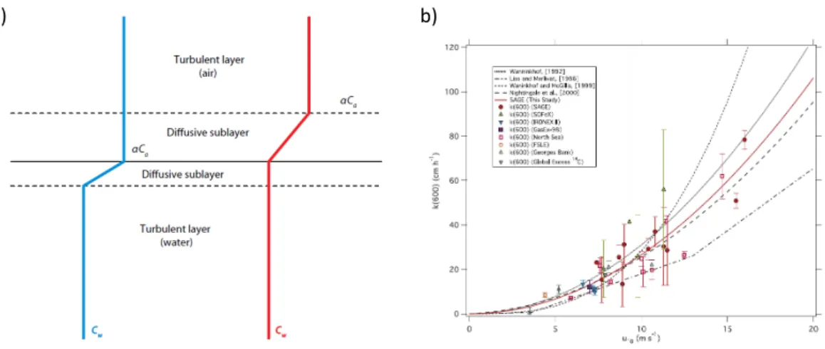
A simple but useful conceptual model to describe air-sea exchange was proposed by Liss
& Slater (1974), which characterizes the interface as the boundary between two diffusive sublayers where turbulence is suppressed and the exchange of mass depends on molecular diffusion (Donelan et al., 2002; Liss & Slater, 1974)(Fig. 1.4a). These layers provide the largest resistance for gases when crossing the interface (Donelan et al., 2002). For insoluble gases like OCS and CS2, the resistance of the air-side diffusive sublayer is several orders of magnitude lower than the water-side resistance, and is thus often neglected in air-sea exchange calculations. For more soluble gases as e.g. DMS, the air-side resistance can become significant at low sea surface temperatures and moderate wind speeds (McGillis et al., 2001).
Air-sea exchange is defined as the product of the concentration gradient across the interface∆c and the transfer velocityk(eq. 1.3).
F =k·∆c (1.3)
While∆c describes the saturation state of the respective compound and thus the direction of the flux, i.e. the thermodynamical component,kdetermines the rate of the exchange, i.e.
the kinetic component (the inverse of the air- and waterside resistance).
A widely used method to calculate air-sea fluxes is the bulk method, where fluxes are calcu- lated from the measured concentration gradient across the surface and a parametrization of the transfer velocityk. This method relies on measurements of the gas in the surface ocean (usually around 5-10m depth) and the marine boundary layer (usually 10-30m height) for
∆c and a parametrization of the transfer velocity, mostly dependent on meteorological
a) b)
Figure 1.4:a) Conceptual model of air sea exchange (from: Wanninkhof et al. (2009)), b) different parameterizations of water-side transfer velocities and spread in measurements with the dual tracer technique (from: (Ho et al., 2006))
parameters such as wind speed. While the method has been extensively tested and generally validated for various gases (see e.g. Garbe et al., 2014; Wanninkhof et al., 2009), it should be noted that both terms,∆c andk, rely on assumptions that may not always be valid:
• The concentration gradient ∆c: When measuring ∆c, concentrations as deep as 6 m in the mixed layer as well as several meters above sea level are taken as representative of the concentration gradient across the air-sea interface. While OCS is generally well mixed in the upper layers of the ocean and the marine boundary layers, it has been shown that this approach has its limitation if strong concentration gradients occur near the surface. Such gradients have previously been inferred for DMS (Kieber et al., 1996; Marandino et al., 2008) and N2O (Kock et al., 2012).
Walker et al. (2016) showed by comparison of direct flux measurements and emissions calculated with the bulk method, that production or enrichment of DMS near the surface can occur under certain meteorological and biological (i.e. blooms of DMS producing plankton species) conditions. In this context, the sea surface microlayer regained attention, as any loss or production occurring there directly influences air- sea exchange, but may be overlooked by the bulk method. The sea surface microlayer may differ from the underlying water in several aspects (Cunliffe et al., 2013) and has been shown to be enriched with chromophoric dissolved organic matter (CDOM) (Wurl et al., 2009), with implications for photochemically produced gases (Zhou &
Mopper, 1997), such as OCS and CS2.
• The transfer velocity k: The transfer velocity is governed by several physical
processes including turbulence, waves, sea spray formation and bubbles, but to date the key parameter and its dependency onk has not been fully characterized. As wind induces turbulence which in turn determines the transfer velocity,khas been found to correlate with wind speed (Liss & Slater, 1974; Wanninkhof et al., 2009).
Therefore, most of the parameterizations forkrely on the wind speed at 10 m height.
These parameterizations have been determined using different techniques such as dual tracer release and eddy covariance and have been tested in wind wave tanks as well as at sea, but uncertainties still exist both in the functional form (linear, quadratic, cubic) and the overall magnitude. Especially at high wind speeds above 10 m s−1,kvalues differ by up to a factor of∼5 (Fig. 1.4b). The scatter in fig. 1.4b indicates that parameters other than wind speed substantially influence the air-sea exchange. A variety of different studies thus investigated the effects of rain (Ho et al., 2004), bubble enhanced gas transfer (Asher & Wanninkhof, 1998; Zhang et al., 2006), surfactants (Frew et al., 1990; Tsai & Liu, 2003) and boundary layer stability (Erickson, 1993). Additionally, it has been questioned that there is only one functional dependence of wind speed andk(i.e. linear, cubic) for all gases, as field measurements point towards differences between e.g. DMS and CO2at wind speeds above 11 m s−1, potentially because of their different solubilities (Bell et al., 2013).
In summary, although the air-sea exchange is a molecular process occurring on vertically very small scales, the horizontal extent of the air-sea interface makes this process glob- ally extremely relevant. Any reduction of uncertainties of the air-sea exchange directly translates into a reduced uncertainty in global marine emission estimates. Increasing our understanding of air-sea exchange is thus crucial for the atmospheric budget of climate relevant trace gases. In addition, the physical and biogeochemical drivers of air-sea fluxes will vary with changing climate, hence an accurate quantification is needed to quantify present and future trace gas emissions and potential feedback mechanisms.
1.3 Marine biogeochemistry of volatile organic sulfur compounds
The ocean plays a major role in the atmospheric budget of the three gases DMS, OCS and CS2(Chin & Davis, 1993; Liss et al., 2014), and it is thus important to accurately quantify their marine emissions in order to assess their influence on climate and atmospheric chemistry. This involves two aspects: First, measurements of the concentration gradient between atmosphere and surface ocean across various oceanic regimes are needed to
determine the order of magnitude of the flux. Second, the key parameters of the marine cycling have to be well understood to upscale observations to a global level. Models with verified parameterizations of production and consumption processes are useful tools for the quantification of emissions. In the following, the current level of understanding of marine production and consumption processes as well as sea surface concentration measurements is reviewed.
1.3.1 Carbonyl sulfide (OCS)
Carbonyl sulfide is present in the surface water of the oceans in the lower picomolar range with strong temporal and spatial variations. Temporal variations on a diurnal as well as on a seasonal scale can vary between super- and undersaturation, with highest concentrations usually shortly after local noon (Kettle, 2000; von Hobe et al., 2003) and during summer (Ulshöfer et al., 1995). Spatial variations are not fully understood due to the limited spatial coverage of previous measurements, but some common patterns seem to emerge. OCS concentrations are usually higher in coastal areas compared to the open ocean (Cutter
& Radford-Knoery, 1993), and higher latitude waters show higher concentrations than tropical or temperate latitudes (e.g. Kettle, 2000; Staubes & Geogrii, 1993). To facilitate the measurements of both spatial and temporal variability of concentrations, automated and continuous measurement systems are needed, which will be addressed within this thesis in chapter 2.
The processes that determine the concentration of OCS in the surface waters have been described previously and include hydrolysis as a loss term, photoproduction and light- independent production as source terms, and air-sea exchange acting as a source or a sink depending on the saturation. Hydrolysis involves the reaction of OCS with either H2O or OH−(reaction 1.4 and 1.5):
OCS+H2O−−−→←−−−H2S+CO2 (1.4) OCS+OH−−−−→←−−−HS−+CO2 (1.5) Hydrolysis rates have been investigated in laboratory and field studies (see section 2.3.1), showing that hydrolysis is strongly temperature dependent. In warm, tropical waters, hydrolysis determines the lifetime of OCS on the order of several hours, whereas in colder waters, lifetime due to hydrolysis can be several days (Elliott et al., 1989).
A photochemical production of OCS was first suggested by Ferek & Andreae (1984) because diurnal variations in the supersaturation of OCS in surface waters follow a similar temporal pattern as solar radiation. The photoproduction of OCS is dependent on the
radiation, the concentration of the precursor and the apparent quantum yield (often also termed in-situ photoproduction rate constant). Flöck et al. (1997) identified cysteine, a common amino acid, as a precursor of OCS in incubation studies, but neither other precursors nor the distribution of these precursors in the ocean is sufficiently well known for modeling purposes. Although several studies used simple models to determine the photoproduction rate constant for specific locations (Uher & Andreae, 1997; von Hobe et al., 2003), no globally valid relationship has been established to date. Incubation experiments at different wave lengths indicated that the apparent quantum yield (AQY) of OCS is strongest in the UV wavelength range (Weiss et al., 1995). However, the variation between published AQYs from the open Pacific ocean (Weiss et al., 1995), the North Sea, and the Gulf of Mexico (Zepp & Andreae, 1994), the Sargasso Sea (Cutter et al., 2004) vary across two orders of magnitude. The inadequate description of photoproduction rates is a shortcoming of previous modeling studies, which hampers an accurate quantification of global marine emissions of OCS.
Light-independent production (also called dark production) has been suggested because OCS concentrations in the absence of light stabilize above the detection limit, indicating that a production process occurs at the same time as the hydrolysis loss process. Experimental studies showed significant production of OCS in the absence of UV light and identified glutathione as a potential precursor (Flöck & Andreae, 1996; Flöck et al., 1997). Currently, two hypotheses exist: a biological process, e.g. microbial activities (Cutter et al., 2004;
Flöck et al., 1997) and/or radical reactions, as Pos et al. (1998) show that in theory, radical formation from metal complexes can lead to the formation of carbonyl sulfide. Dark production has been shown to vary with temperature and CDOM content, but currently only one parameterization describing dark production is available, which is based on data from several cruises to the Atlantic ocean (Von Hobe et al., 2001).
Under- and supersaturation of OCS has been detected in surface waters (Kettle, 2000;
Ulshöfer et al., 1995), which implies that exchange of OCS across the air-sea interface occurs in both directions. Uncertainties related to this process are similar to other trace gases whose emissions are derived with the bulk method (see section 1.2).
In total, the production and loss processes for OCS are reasonably well described to narrow down the key parameters influencing surface concentrations and thus emissions.
However, insufficient quantification of both production processes has still introduced consid- erable uncertainty in global modeling efforts to simulate global sea surface concentrations and emissions of OCS.