Deciphering the variability in Mg/Ca and stable oxygen isotopes of individual foraminifera

This article has been accepted for publication and undergone full peer review but has not been through the copyediting, typesetting, pagination and proofreading process which may lead to differences between this version and the Version of Record. Please cite this article as doi: 10.1029/2018PA003533

Groeneveld Jeroen (Orcid ID: 0000-0002-8382-8019) Mackensen Andreas (Orcid ID: 0000-0002-5024-4455) Laepple Thomas (Orcid ID: 0000-0001-8108-7520)

Deciphering the variability in Mg/Ca and stable oxygen isotopes of individual foraminifera

Groeneveld, Jeroen^*1,2, Sze Ling Ho^1,3, Andreas Mackensen⁴, Mahyar Mohtadi², Thomas Laepple¹

1Alfred Wegener Institute, Helmholtz Center for Polar and Marine Research, Telegrafenberg A45, D- 14473 Potsdam, Germany

2MARUM-Center for Marine Environmental Sciences, University of Bremen, Klagenfurter Strasse 2-4, D-28359 Bremen, Germany; *corresponding author (jgroeneveld@uni-bremen.de)

3now at Institute of Oceanography, National Taiwan University, 10617 Taipei, Taiwan

4Alfred Wegener Institute, Helmholtz Center for Polar and Marine Research, Am Alten Hafen 26, D- 27568 Bremerhaven, Germany

Keywords: Mg/Ca, ¹⁸O, planktic foraminifera, individual foraminifer analyses, climate variability Key Points

- Variability in Mg/Ca and ¹⁸O of individual foraminifer analyses (IFA) shows a strong relationship suggesting a common factor of influence

- Temperature is identified as the main common factor controlling both proxies supporting the use of IFA to reconstruct climate variability

- The weak relationship of the IFA data to seasonal and interannual variability suggests that ecology plays an important role

Abstract

Foraminifera are commonly used in paleoclimate reconstructions as they occur throughout the world’s oceans and are often abundantly preserved in the sediments. Traditionally, foraminifera- based proxies like ¹⁸O and Mg/Ca are analyzed on pooled specimens of a single species.

Analysis of single specimens of foraminifera allows reconstructing climate variability on timescales related to El Niño-Southern Oscillation (ENSO) or seasonality. However, quantitative calibrations between the statistics of individual foraminiferal analyses (IFA) and climate variability are still missing. We performed Mg/Ca and ¹⁸O measurements on single specimens from core-top sediments from different settings to better understand the signal recorded by individual foraminifera. We used three species of planktic foraminifera (G. ruber (s.s.), T.

sacculifer, and N. dutertrei) from the Indo-Pacific Warm Pool (IPWP) and one species (G. ruber (pink)) from the Gulf of Mexico (GoM). Mean values for the different species of Mg/Ca vs calculated ¹⁸O temperatures agree with published calibration equations. IFA statistics (both mean and standard deviation) of Mg/Ca and ¹⁸O between the different sites show a strong relationship indicating that both proxies are influenced by a common factor, most likely temperature variations during calcification. This strongly supports the use of IFA to reconstruct climate variability. However, our combined IFA data for the different species only show a weak relationship to seasonal and interannual temperature changes, especially when seasonal variability increases at a location. This suggests that the season and depth habitat of the foraminifera strongly affect IFA variability, such that ecology needs to be considered when reconstructing past climate variability.

1. Introduction

Foraminifera are commonly used in paleoclimate reconstructions as they occur throughout the world’s oceans and are easily preserved in the sediments. Traditionally, proxies like stable oxygen isotopes and Mg/Ca are analyzed on samples consisting of many pooled specimens of a single species. As a typical sediment sample includes the recordings of several up to hundreds or even thousands of years but a single specimen only lived and recorded several weeks, a larger number of 10-100 specimens is needed to provide a representative signal of the paleoclimatic parameter that is to be reconstructed (Schiffelbein & Hills, 1984; Rosenthal et al., 2000; Nürnberg, 2000; Lea, 2004;

Katz et al., 2010; Laepple & Huybers, 2014). In the early eighties it was already shown that the variation in stable isotope values in single specimens (individual foraminifera analysis = IFA; also

known as single specimen analysis (SSA), individual specimen analysis (ISA) or single foraminifer analysis (SFA) (e.g. Wit et al., 2010; Thirumalai et al., 2013; Metcalfe et al., 2015)) from the same sediment sample was much larger than expected from just long-term temperature variations (Killingley et al., 1981; Schiffelbein & Hills, 1984). This was linked to varying water depths of calcification for different specimens and used by Schiffelbein and Hills (1984) to estimate the uncertainty of analyses commonly performed on pooled specimens. Many studies then investigated additional factors that can impact variations in single shell ¹⁸O, including bioturbation (Billups &

Spero, 1996; Stott & Tang, 1996), interspecific shell ontogeny (Spero & Williams, 1990), photosymbiont influences (Spero & Lea, 1993; Houston et al., 1999), seasonal salinity changes (Spero & Williams, 1990; Tang & Stott, 1993), discrepancies between living and recently fossilized individuals (Waelbroeck et al., 2005), or genetic differences within the same morphospecies (Morard et al., 2016; Sadekov et al., 2016). More recently, it was suggested that this variation within the same sample can be linked to shorter timescale climate variability related to ENSO (Koutavas et al., 2006; Leduc et al., 2009; Khider et al., 2011; Scroxton et al., 2011; Sadekov et al., 2013; Rustic et al., 2015) or the seasonal cycle (Wit et al., 2010; Ganssen et al., 2011; Metcalfe et al., 2015; Vetter et al., 2017). These studies used analyses of stable oxygen isotopes (¹⁸O) on individual foraminifera from the same sediment samples to determine short-term variations. However, to what extent the IFA variations in ¹⁸O are suitable to reconstruct past climate variability, is still an open question.

Assessing different parameters of the same sample may help to identify a common driving factor of IFA variability. Mg/Ca and ¹⁸O are analyzed on the same biotic carrier and therefore differences in season and habitat are avoided in the proxy signal recorded by the foraminiferal tests (Nürnberg, 2000). ¹⁸O is already routinely measured on single specimens, but Mg/Ca in individual foraminifera has mainly been analyzed by Laser Ablation ICP-MS. Laser ablation has been instrumental in demonstrating that trace elements are heterogeneously distributed throughout tests related to banding during biomineralization or the deposition of primary vs. secondary calcite (Eggins et al., 2004; Sadekov et al., 2008; Hathorne et al., 2009; Wit et al., 2010; Spero et al., 2015). Additionally, the effects of diagenesis can be identified by laser ablation (Groeneveld et al., 2008; Van Raden et al., 2011). Despite the advantage of laser ablation analyses for determining intra-test variability, it takes many laser profiles to give a representative signal in order to be directly compared to IF analyses of ¹⁸O (De Nooijer et al., 2014).

Flow-Through time resolved analysis and automated cleaning provides an alternative for the rigorous manual cleaning of samples for Mg/Ca (Haley & Klinkhammer, 2002). Samples are placed on a filter and then connected to an automated cleaning device, which reduces the loss of sample material during the cleaning process. This allows the analysis of trace metal/Ca in individual foraminifera (Haarmann et al., 2011), very small samples (McKay et al., 2015), or to separate diagenetic and primary calcite (Klinkhammer et al., 2009).

In this study we analyze the Mg/Ca of individual foraminifera using Flow-Through automated cleaning and analyze ¹⁸O on individual foraminifera from the same sediment sample. This dual approach allows us to explore whether the spread between single measurements in individual foraminifera is related to environmental parameters and hence climate (e.g. seasonality), or is rather dominated by analytical and processing uncertainties. We use four species of planktic foraminifera (Globigerinoides ruber (sensu stricto (s.s.)), G. ruber (pink), Trilobatus sacculifer, and Neogloboquadrina dutertrei) from core top sediments representing a range of oceanic conditions.

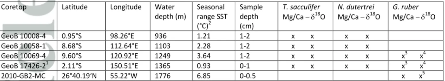
Core tops originate from the Indo-Pacific Warm Pool, both from the warm pool and from upwelling- affected areas, and from the Gulf of Mexico, which experience seasonal variations in sea surface temperature (SST) between 1°C and 7°C (Table 1). We analyze for the first time combined individual foraminifer (IF) Mg/Ca and ¹⁸O both on single specimens from the same samples and show that these independent parameters show similar distributions. As the sample processing and analytics are different for both proxies, this provides strong evidence for a common climatic origin of the Mg/Ca and ¹⁸O signal. We further show that their distributions cannot be explained solely by seasonal or interannual temperature variations but are likely also related to changing habitat preferences and/or oceanographic conditions.

2. Oceanographic and ecological setting

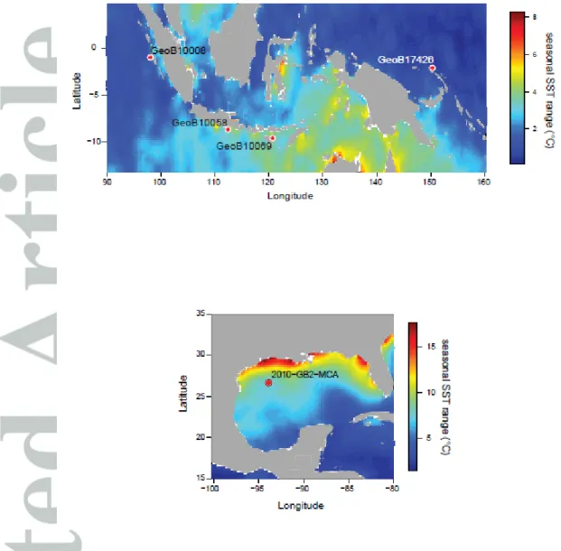
Core top locations were selected based on particular oceanic conditions to include a wide range of settings (Figure 1) in terms of variability experienced. We selected one location from the Western Pacific Warm Pool (WPWP) just north of Papua New Guinea (PNG), three locations along the western coast of Indonesia (Northern Mentawai Basin (NMB), Lombok Basin (LB), and Savu Sea (SS)), and one location from the Gulf of Mexico (Figure 1). The main varying characteristic between these locations is seasonality in seawater temperatures. The PNG and NMB locations are typical warm pool sites with low seasonality in temperature (seasonal range in SST ~1°C; Table 1; Figures 1 and 2), oligotrophic conditions, and a deep thermocline, although the NMB does experience significant

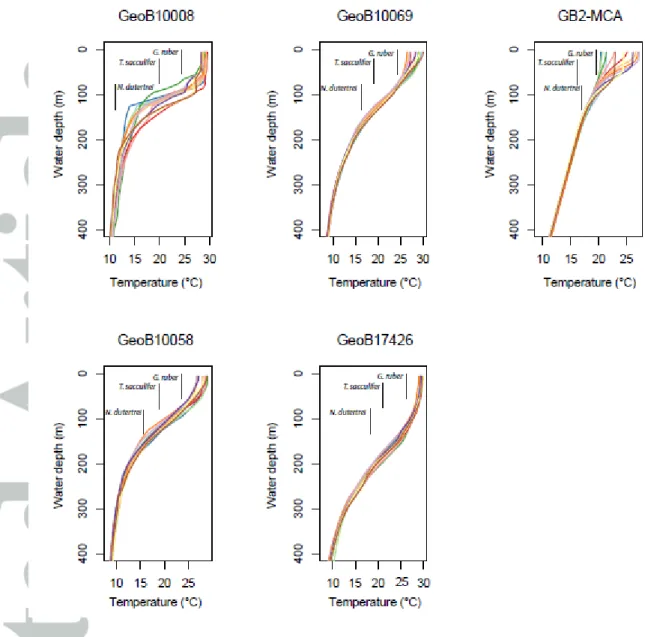
subsurface temperature variability (Mohtadi et al., 2011). The Lombok Basin and Savu Sea are also part of the IPWP but experience stronger seasonal changes in SST (~2-4°C; Table 1; Figure 2) and thermocline-depth during the austral winter when the southeast monsoon causes Ekman-induced upwelling (Table 1; Mohtadi et al., 2011). Calcification depth of T. sacculifer is within the mixed layer varying between 40 and 95 m in the WPWP and between 20 and 50 m off Indonesia (Mohtadi et al., 2011; Hollstein et al., 2017). Although N. dutertrei occurs throughout the year, the maximum flux of specimens occurs during the upwelling season off Indonesia, and its estimated habitat depth varies between 75-100 m, while in the WPWP it varies between 90-160 m (Mohtadi et al., 2011; Hollstein et al., 2017).

The location in the GoM was selected because of its large seasonality. Seasonal surface temperature and salinity variations of up ~7°C (Table 1) and 0.23 salinity units, respectively, occur because the seasonal migration of the Intertropical Convergence Zone (ITCZ) moves the warm Loop Current into the GoM during boreal summer, while during boreal winter the southward migration of the ITCZ keeps the Loop Current outside of the GoM (Poore et al., 2013). Globigerinoides ruber (pink) is one of the dominantly present foraminifer species in the GoM and occurs throughout the year but with highest fluxes generally during the warm season (Poore et al., 2013). The habitat depth of G. ruber is generally within the upper 50 m of the water column. In this study we analyzed only Globigerinoides ruber (pink) in the GoM as the abundance of G. ruber (s.s.) was insufficient.

3. Methods and Material

The core tops from the IPWP were collected during the R/V SONNE 228 (GeoB 17426-2; Mohtadi et al., 2013) and R/V SONNE 184 (GeoB 10008-4, GeoB 10058-1, and GeoB 10069-4; Hebbeln et al., 2005) expeditions (Table 1). The core tops off Indonesia were AMS-¹⁴C dated as modern (>1950 AD) (Mohtadi et al., 2011). Core top GeoB 17426-2 has a calibrated AMS-¹⁴C age of 309 yr BP (Table 1).

Core top 2010-GB2-MC from the Gulf of Mexico was collected in Summer 2010 on the R/V Cape Hatteras, and was AMS-¹⁴C dated as modern (>1950 AD) (Thirumalai et al., 2018).

The planktic foraminiferal species Globigerinoides ruber (s.s.), G. ruber (pink), Trilobatus sacculifer (without sac-like final chamber), and Neogloboquadrina dutertrei (dextral) were picked for the analysis of stable oxygen and carbon isotopes, and Mg/Ca. All foraminifera were picked from the 315-400 µm size fraction. For IFA of Mg/Ca, one specimen per analysis was used for T. sacculifer and N. dutertrei, and two specimens for G. ruber due to the smaller amount of calcite per specimen.

Using two specimens per analysis reduces the standard deviation and expected range by √𝑛, where

n is the number of specimens used in the samples, in this case n = 2. After rescaling with this factor of ~1.4, the two specimen analysis can be compared with the single specimen analyses of T.

sacculifer and N. dutertrei. For simplicity, if not stated otherwise, all values in the text, table and figures are rescaled to represent the statistics of single specimen analyses and we call all the analyses (whether based on two or single specimen) single specimen analyses.

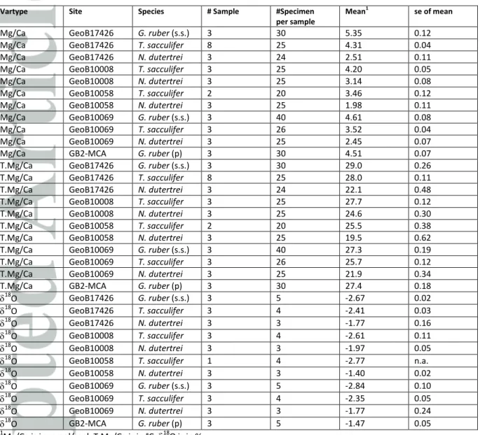
For pooled analyses of Mg/Ca, 25 specimens per sample were used for T. sacculifer and N. dutertrei, and 40 specimens for G. ruber. For stable oxygen isotopes, three-four specimens for N. dutertrei, four-five specimens for T. sacculifer, and five-six specimens for G. ruber were used for the pooled samples respectively, while for IFA one specimen per sample was used for T. sacculifer and N.

dutertrei, and two specimens for G. ruber were needed to have enough material for analysis.All data presented here are stored in the Pangaea database (www.pangaea.de).

3.1 Mg/Ca

After gentle crushing, the shell fragments of the pooled samples were cleaned according to the standard cleaning protocol for foraminiferal Mg/Ca analyses (Barker et al., 2003). After dissolution, samples were centrifuged for 10 minutes (6000 rpm) to exclude any remaining insoluble particles from the analyses. Samples were diluted with Seralpur before analysis with an ICP-OES (Agilent Technologies, 700 Series with autosampler ASX-520 Cetac and micro-nebulizer) at MARUM, University of Bremen. Instrumental precision of the ICP-OES was monitored every five samples by analysis of an in-house standard solution with a Mg/Ca of 2.93 mmol/mol (long-term standard deviation of 0.026 mmol/mol or 0.88%). The ECRM752-1 limestone standard, with a reported Mg/Ca of 3.75 mmol/mol, was analyzed (n = 44) to allow inter-laboratory comparison (Greaves et al., 2008) with an average of 3.85 + 0.027 mmol/mol.

A total of 451 foraminifera were gently crushed for individual shell analyses after each single foraminifer was placed on a polypropylene filter with a PTFE membrane (0.45 µm mesh; Whatman) using a pipette tip. The filters were connected to a Flow-Through – Automated Cleaning Device (Klinkhammer et al., 2004; Haarmann et al., 2011). Cleaning over a filter reduces the loss of material, which occurs with traditional cleaning, allowing the analysis of single specimens. The automated cleaning involves three rinses of 10 minutes each with Seralpur, 1%-NaOH buffered H2O2 for oxidation, and Seralpur. Several drops of NH3 (suprapur) were added to the Seralpur to increase the pH to prevent leaching during the Seralpur rinses. For oxidation, the filters were placed in a water bath at 98°C. After the cleaning, the filters were connected to a cleaned syringe with 1 mL of 0.075 M QD HNO3 to dissolve the foraminiferal fragments by placing the syringes in a rack and letting the

acid slowly drop through the sample to allow enough time for dissolution. Samples were analyzed with an ICP-OES (Agilent Technologies, 700 Series with autosampler ASX-520 Cetac and micro- nebulizer) at MARUM, University of Bremen. In comparison with the pooled samples the analytical method was tuned to the lower concentrations of single specimen samples, i.e., calibration samples with lower concentrations, and a more sensitive element line for Al (167.019 nm) (see below for details). Combined analytical precision for all species and locations based on three repetitions for each sample analysis for the IFA was 0.55% for Mg/Ca (n = 451).

Temperatures for the different species were calculated using the species dependent calibrations from Anand et al. (2003; Mg/Ca = B * exp (A*T), with B = species specific, and A = 0.09 (assumed based on the findings of previous calibration studies (Elderfield and Ganssen, 2000)). For the main conclusions of this study, only the exponential constant of A = 0.09 is relevant as the pre-exponential constant B does not influence the resulting temperature spread from the IFA distribution.

We set thresholds to classify IF analyses as reliable depending on the amount of material and possible contamination. As the analysis of single foraminifera approaches the limits of the amount of material which can be measured on the ICP-OES, we set a conservative minimum threshold of 4 ppm Ca for an acceptable measurement (Figure S1). Potential contamination by remaining clay particles was monitored using Al/Ca. Because the absolute concentrations were close to the detection limit, the absolute values of the Al/Ca may be too high due to matrix effects. Therefore, we set a threshold of 2 mmol/mol for Al/Ca above which samples are classified as possibly contaminated and not included in further statistical analyses. After applying both thresholds, 286 samples remain. The sensitivity of the results on the Ca and Al/Ca thresholds was tested, showing that our choice is a reasonable tradeoff between minimizing the effect of potential contamination and not removing too many measurements (Figure S1). To ensure that the FT system did not get contaminated by remaining particles during the cleaning, the system was regularly rinsed with 1M HNO3 (3 min.) followed by buffered Seralpur (20 min.), and after the analysis of each sample was finished the tubes were rinsed with Seralpur (10 min.). Blank samples (n = 41), which both received the same cleaning treatment as regular samples and which were taken from specific positions along the FT-device (e.g.

at the end of a particular tube), were regularly analyzed and had element concentrations below the detection limit for each element. The blank samples were not additionally acidified before analysis.

3.2 Stable isotopes

Stable oxygen isotope analyses on pooled samples were performed on a Finnigan MAT 252 mass spectrometer equipped with an automated carbonate preparation device at MARUM, University of Bremen. Isotopic results were calibrated relative to the Vienna Pee Dee belemnite (VPDB) using the NBS19 standard. The standard deviation of the laboratory standard was lower than 0.07‰ for the measuring period.

Stable oxygen and carbon isotope analyses (¹⁸O and ¹³C) on individual foraminifera (n = 506) were performed using a Finnigan MAT 253 mass spectrometer with the automated carbonate preparation device Kiel IV at AWI Bremerhaven. The precision of the stable oxygen isotope analyses determined on an internal laboratory standard, measured over a one-year period together with the samples, was better than 0.08‰. Values are reported in -notation relative to Vienna Pee Dee Belemnite (VPDB), calibrated by using the National Institute of Standards NBS 18 and 19 standards. Samples with a sample-intensity of less than 2000 mV were excluded due to insufficient material, leading to 483 remaining samples. Although instrument-specific and therefore not commonly applicable we tested the dependency of the results on the sample intensity threshold to show that the standard deviation of the IFA variability is insensitive to this choice (Figure S2).

3.3 Statistical methods

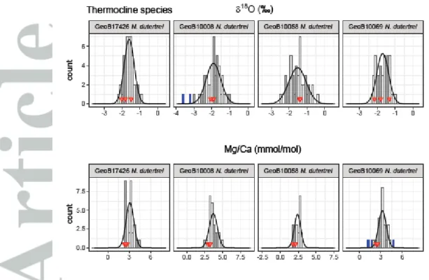
Despite removing samples that had a too-low amount of sample material left for analysis or a potential threat of contamination as described above, outliers related to the presence of a higher portion of secondary crust on N. dutertrei or other unknown reasons are still possible. Therefore, we removed outliers in the Mg/Ca and ¹⁸O data using the 1.5x IQR (interquartile range) criterion, a robust method for outlier detection (Tukey, 1977). This criterion removed six (2.0%) of the single specimen samples for Mg/Ca and seven samples for ¹⁸O (1.5%; Figure 3). Our main conclusions are insensitive to this outlier removal (Figures S1 and S2).

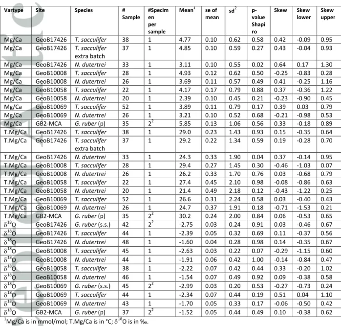
To estimate the skewness of the IFA distributions we use the Fisher-Pearson coefficient of skewness and provide bootstrap confidence intervals as the classical confidence intervals were shown to be unreliable (Wright & Herrington, 2011). We test the IFA distributions for normality using the Shapiro- Wilk test (Shapiro & Wilk, 1965). In only one of 20 cases (Mg/Ca GeoB17426, N. dutertrei), the null hypothesis that the data are normally distributed (p = 0.05) is rejected (Table 2). When omitting the outlier correction, four of the 20 distributions get rejected, consistent with the visually apparent outliers in these distributions (¹⁸O: GeoB10069 G. ruber (s.s.), GeoB10008 T. sacculifer; Mg/Ca:

GeoB17426 T. sacculifer, GeoB10058 T. sacculifer). We therefore conclude that there is no evidence for a non-normal distribution and characterize the spread of the IFA using the standard deviation and provide the analytical confidence intervals of the standard deviation based on the ChiSquare distribution. We note that the normality test may be too optimistic for G. ruber as the measurements were performed on two specimens and this will reduce any higher moments of the distribution such as the skewness.

We use a bias corrected estimator for the standard deviation that assumes a normally distributed random variable (Brugger, 1969). The bias correction is only relevant for the comparison of the pooled and IFA spread but has no discernible effect on the analysis of the IFA variability as the sample sizes are large enough (>30 individuals).

3.4. Oceanographic data and expected proxy variability

We use the monthly climatological seawater temperature and salinity from the World Ocean Atlas (WOA) 2013 on a 1x1 degree grid (Locarnini et al., 2013; Zweng et al., 2013). To estimate the effect of interannual variations on the expected proxy variability, we use annual seawater temperature and salinity from the NCEP Global Ocean Data Assimilation System (GODAS) (Behringer & Xue, 2004).

We further use the global gridded data set of the oxygen isotopic composition in seawater (Version 1.1) (LeGrande & Schmidt, 2006) to extract the ¹⁸Osw at the core positions. Even though most of our core-tops are dated as modern, the time period recorded by the foraminifera is likely not the same as the time period represented by the oceanographic data. However, in contrast to a warming trend in the last decades, the change in variability is expected to be minor and discrepancies in the recorded time period should thus have no discernable influence on our results.

To estimate the effect of seasonal and interannual variations on ¹⁸Osw, we predicted the ¹⁸Osw

anomalies from the monthly WOA and annual GODAS salinity anomalies. For this step, we assumed a linear relationship between both variables with a slope of 0.257‰/psu for the GoM (Spero &

Williams, 1990) and 0.42‰/psu for the remaining sites (Morimoto et al., 2002). For simplicity, we extracted the ¹⁸Osw and temperature at fixed species dependent water depth ranges (G. ruber (s.s.) and G. ruber (pink) at 0-50 m, T. sacculifer at 20-70 m and N. dutertrei at 80-120 m) but we confirmed that our results are not sensitive to the use of site-specific depth ranges (Regenberg et al., 2009; Mohtadi et al., 2011; Hollstein et al., 2017; not shown). As interannual and seasonal variability are largely independent, we approximate the total variability expected to influence the single

specimen as 𝑠𝑑_{𝑡𝑜𝑡𝑎𝑙} = √𝑠𝑑_{𝑠𝑒𝑎𝑠𝑜𝑛𝑎𝑙}²+ 𝑠𝑑𝑖𝑛𝑡𝑒𝑟𝑎𝑛𝑛𝑢𝑎𝑙2

. Testing this approximation with monthly SST data shows that deviations from the true variability at our study sites are less than 20%.

Isotopic calcification temperatures of the foraminifera were calculated, using the paleotemperature equation from Bemis et al. (1998), from measured ¹⁸O (from the planktic foraminifera in VPDB units) and estimates of ¹⁸Osw (in SMOW units):

T = 14.9 - 4.8*(¹⁸O - (¹⁸Osw - 0.27))

4. Results and Discussion

4.1 Variability in single specimen Mg/Ca and ¹⁸O

Individual foraminifer Mg/Ca values for T. sacculifer varied between 2.50 and 6.24 mmol/mol with an average of 4.38 mmol/mol (Figure 3; Table 2). Assuming that temperature calibrations based on pooled specimens can also be applied to single specimens, this translates into a range between 22.0 and 32.1°C (average = 28.0°C). Individual foraminifer Mg/Ca values for N. dutertrei varied between 1.64 and 4.93 mmol/mol (17.4-29.6°) with an average of 3.14 mmol/mol (24.3°C); and for G. ruber (pink) between 4.39 and 7.50 mmol/mol (27.1-33.0°C) with an average of 5.85 mmol/mol (30.2°C).

As two specimens per sample were used for G. ruber (pink), the range is ~1.4 times less than expected for single specimen analyses. The average values are all higher than the average Mg/Ca of the pooled specimen analysis for each respective species (T. sacculifer: 4.38 vs 4.03 mmol/mol; N.

dutertrei: 3.14 vs 2.52 mmol/mol; G. ruber (pink): 5.85 vs 4.51 mmol/mol) (Table 3). The results show that the single specimen Mg/Ca values for all three species are close to normally distributed as the Shapiro-Wilk test rejected the null-hypothesis for only one of the distributions (Mg/Ca GeoB17426, N. dutertrei) (Figure 3; Table 2).

An additional, replicate batch of 59 IFA (37 samples after concentration thresholding and outlier removal) was performed using T. sacculifer specimens from GeoB 17426-2 which included an extra, short ultrasonic bath step before the FT-cleaning. Comparison between both batches shows that the mean (4.85 vs. 4.77 mmol/mol using the standard procedure), standard deviation (0.59 vs. 0.62) and skewness (0.43 vs. 0.42) are statistically indistinguishable from the sample set prepared using the standard procedure (Table 2). This suggests that the cleaning process for IFA was sufficient to extract the primary signals, and underlines the robustness of the IFA statistics when conservatively removing samples with too-low concentrations or signs for potential contamination.

For stable oxygen isotopes of the single specimens a total of 476 samples were included in further analyses after intensity screening and outlier removal. For T. sacculifer, ¹⁸O varied between -1.16 and -3.23‰ with an average of -2.40‰ (Figure 3a; Table 2; Supplements). G. ruber (s.s.) and G. ruber (pink) ¹⁸O varied between -2.33 and -3.40‰ with an average of -2.87‰ and between -0.97 and - 2.15‰ with an average of -1.52‰, respectively (Figure 3a; Table 2). As for Mg/Ca, the range in values is ~1.4 times less than expected for single specimen analysis because two specimens were analyzed per sample. For the thermocline-dwelling N. dutertrei, the spread in ¹⁸O was between - 0.44 and -2.97‰ with an average of -1.68‰ (Figure 3b; Table 2). Because no different preparation techniques are performed as with Mg/Ca, the average ¹⁸O values for single specimens are similar to the average ¹⁸O for pooled specimen samples for each species (Table 3). There is no indication that the ¹⁸O values for the respective samples are not normally distributed (Table 3). The skewness of the distributions ranges from -0.29 to 0.51, but is only significantly different from zero for the distribution in one sample (GeoB10069 T. sacculifer, skewness = 0.51).

Because stable carbon isotopes are affected by many additional factors than just temperature, we did not include them in the discussion but only show them in the Supplements (Figure S3) and the data are available via Pangaea.

4.2 Comparing pooled vs. single specimen analyses; Mean values 4.2.1 Mg/Ca

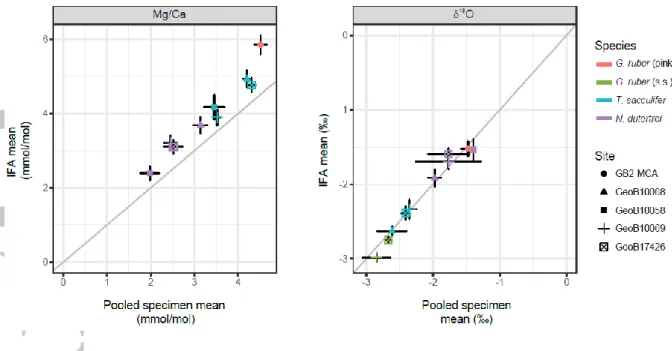
Average Mg/Ca of the individual foraminifera for each species and core top is on average 0.66 mmol/mol (~1.9°C) higher than for the pooled specimen samples (Figure 4; Table 3). The smallest difference was found for T. sacculifer in GeoB 10069-4 (0.37 mmol/mol or ~0.9°C), and the largest difference was for G. ruber (pink) in GB2-MCA (1.34 mmol/mol or ~2.84°C). The relatively constant offset between both approaches points to a systematic difference possibly due to sample preparation.

As individual and pooled specimens are picked from the same samples and are indistinguishable for

¹⁸O, the differences have to be caused by the different cleaning and measurement process. The analyses of the consistency standards, which were diluted to reflect typical IF and pooled specimen concentrations, show the same values excluding evidence for instrumental drift, i.e. between IF or pooled sample, or specific bias in the Mg/Ca measurements themselves suggesting that the

differences stem from the cleaning protocols. Possibilities include either a too intense cleaning of the samples with pooled specimens, or remaining contamination on single foraminifera.

Previous cleaning experiments have shown that with more intense cleaning, the higher Mg-parts of the tests are more affected by dissolution thus lowering Mg/Ca (Brown & Elderfield, 1996; Rosenthal et al., 2000; Barker et al., 2003; Regenberg et al., 2006); for example adding a reduction step to the cleaning resulted in 1-2°C lower temperatures (Barker et al., 2003; Rosenthal et al., 2004). The main reason to use a FT cleaning device in the current study was to reduce the loss of material during the cleaning process, which normally occurs during the manual cleaning, thus making the cleaning procedure less intense. Accordingly, it can be expected that when no material is lost the resulting Mg/Ca may be slightly higher than the traditionally cleaned samples of pooled specimens. This implies that a FT-specific Mg/Ca vs temperature equation needs to be calibrated for optimum precision when Mg/Ca paleotemperature records are reconstructed using FT-preparation.

The higher IFA Mg/Ca may also have been caused by a less efficient cleaning of the FT method. After cleaning, the samples were dissolved by running the dissolution acid over the samples. This may have led to the inclusion of some <0.45 µm particles, which could have been freed by the dissolution of the calcite. However, we already removed samples with suspiciously high Al/Ca from further discussion (Figure S1). And additional evidence that the samples were clean comes from the extra batch of samples for which an extra cleaning step, i.e. ultrasonic treatment, was performed and which shows the same mean and standard deviation as the first batch (Table 2).

We compare the replicate pooled specimen and single specimen variability of all species to infer the origins of the single specimen variability. In the case of no measurement uncertainty, the spread of the pooled specimen samples after adjusting for the number of tests in each sample by multiplying with √𝑛, where n is the number of foraminifera per sample, should be similar to the spread of the single specimen samples. The mean spread for the different species in Mg/Ca of the single specimen samples is 0.7 mmol/mol, similar to the mean spread of the pooled specimen samples of 0.75 mmol/mol after adjusting for the number of tests in each sample. This confirms for Mg/Ca that variations in the foraminiferal Mg/Ca and not analytical uncertainties are the main driver for the replicate variability.

4.2.2 Stable oxygen isotopes

The mean ¹⁸O from the pooled specimen samples and mean ¹⁸O of the IFA are indistinguishable within their statistical uncertainty in spite of differences in sample size and instruments used (Figure

4). The overall mean value of ¹⁸O of the pooled specimen samples of -2.13‰ differs from the overall mean values of the single specimen ¹⁸O samples by less than 0.01. This reproducibility also applies when comparing the means for every species and every site specifically (Figure 3, 4; Table 3).

As the samples for pooled specimen analyses consisted only of three to six specimens, the mean IFA values based on the values of ~40 separate specimens are the more reliable estimates of the true

¹⁸O value.

As we typically measured three replicate samples of pooled specimens with three to six foraminiferal tests in each sample as well as the measurements of typically ~40 individual foraminifera, we can compare the replicate pooled specimen and IFA variability similar to the comparison for Mg/Ca. The mean spread for the different species for single specimen samples of 0.33‰ is similar to the adjusted mean spread of the pooled specimen samples of 0.27‰ providing confidence that the signal and not the measurement process dominates the ¹⁸O variability.

4.3 Comparison of ¹⁸O vs. Mg/Ca with pooled specimen calibrations

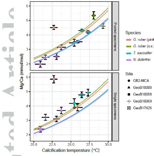
We compare the calcification temperatures calculated from the measured ¹⁸O with the mean Mg/Ca values calculated from the pooled specimen and the single specimen measurements (Figure 5). For ¹⁸O we combine the pooled specimen and the single specimen measurements to one mean value, as both are indistinguishable, and the pooled specimen samples contain too few specimens to deliver reliable mean ¹⁸O values.

For both IF and pooled specimens, the mean Mg/Ca to calcification temperature relationship follows existing species-specific calibrations (Anand et al., 2003; Figure 5). In general, the pooled specimen values are consistent with the standard calibrations as expected, as this follows the commonly applied procedure. As discussed previously (Section 4.2.1), the IF mean values are slightly higher than the pooled specimen mean and thus slightly above the calibration curve. For both pooled specimen and single specimen Mg/Ca, the GoM G. ruber (pink) values deviate from the expected relationship by 1.3‰ for pooled specimens and 1.7‰ for single specimens. While the gridded dataset (LeGrande & Schmidt, 2006) suggests a value of 0.7‰ at the core position, observational data suggest values up to 1.9‰ for the northern Gulf of Mexico (Grossman & Ku, 1986; Surge &

Lohmann, 2002) and could thus resolve the discrepancy from the calibration relationship.

Estimating an own calibration equation from the IFA data by excluding the Gulf of Mexico site results in an exponential constant of 0.096 + 0.011 (1 se), thus statistically indistinguishable from the

standard calibration slope of 0.09 (Anand et al., 2003). This result also holds when using the Shackleton (1974) equation for the ¹⁸O to temperature relationship. However, the intercept is sensitive to the calibration equation and using the Shackleton (1974) equation leads to pooled specimen values being below the calibration lines and IFA values matching the calibration relationship (not shown).

4.4 Variability in individual foraminifer analyses

The spread in IFA is often interpreted as climate variability (Koutavas et al., 2006; Leduc et al., 2009;

Khider et al., 2011; Ganssen et al., 2011; Metcalfe et al., 2015; Vetter et al., 2017). As temperature is the main driver at our sites for both Mg/Ca and ¹⁸O, we expect that both Mg/Ca and ¹⁸O IFA should show similar variability when accounting for their respective temperature calibrations.

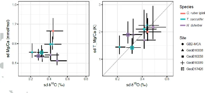
Indeed, using an exponential constant of 0.09 results in a mean TMg/Ca spread (1 sd + 1 se) of 1.8 + 0.2°C and a mean ¹⁸O spread of 0.37 + 0.04‰, thus a ratio sd (TMg/Ca) to sd (¹⁸O) of 5.1 + 0.8 (1 se).

Similar results (ratio of 4.5 – 5.6) are obtained when analyzing each species separately. The similarity of this ratio with the published ¹⁸O sensitivity on calcification temperature (e.g. 4.8 for Bemis et al., 1998) strongly supports that both signals are largely driven by variability in the calcification temperature and thus encouraging for the use of IFA as a climate proxy.

Comparing the site-specific IF Mg/Ca and ¹⁸O variability after converting Mg/Ca to temperature units (Figure 6, right panel) shows that the TMg/Ca and δ¹⁸O variability scatter around the slope of 4.8 as expected from the sensitivity of δ¹⁸O to temperature during calcification (Shackleton, 1974; Bemis et al., 1998; Bouvier-Soumagnac & Duplessy, 1985). The variability of both proxies shows a statistically significant positive correlation (R = 0.75, p = 0.02). Interestingly, this relationship largely breaks down when comparing the Mg/Ca and ¹⁸O variability before calibration, showing the importance of the nonlinear (exponential) Mg/Ca to temperature relationship that leads to a different scaling of TMg/Ca to Mg/Ca variability depending on the mean temperature. Additionally, the intercept is only slightly positive, which also suggests that the majority of Mg/Ca and ¹⁸O variability is dominated by the same mechanism. This also shows that the effect of salinity on the variability of the ¹⁸O signal is limited, consistent with the expected variability predicted from the oceanographic data (not shown).

Analyzing surface dwellers and thermocline dwellers separately supports our finding (Figure S4) but also shows that the relationship for thermocline dwellers is more sensitive to the outlier definition.

Although the number of samples is too small to draw a robust conclusion, this might indicate that

the analysis on single N. dutertrei specimens is more challenging (see also section 4.5), potentially also as N. dutertrei, in contrast to T. sacculifer and G. ruber, builds a secondary crust later in the life cycle. This crust is thought to form deeper in the water column recording lower temperatures. This was also shown for other deeper-dwelling foraminifera with a distinction between higher Mg/Ca in the primary calcite and lower Mg/Ca in the crust (Hathorne et al., 2009; Groeneveld & Chiessi, 2011;

Jonkers et al., 2012; Steinhardt et al., 2014). Although only specimens of N. dutertrei without an obvious crust were selected, the formation of a crust is gradual such that it cannot be avoided that some specimens contain some crust. This would skew the analyses of either one of the proxies towards “colder” values preventing a linear relationship between the averages from different locations (Figure S4). The relationship between the variability displayed by Mg/Ca and ¹⁸O also argues against a strong influence of vital effects (De Nooijer et al., 2014) or genetic variations (Morard et al., 2016; Sadekov et al., 2016) on the variability of Mg/Ca and δ¹⁸O in single specimens.

These mechanisms could only explain our findings by simultaneously influencing δ¹⁸O and Mg/Ca with the relative amount of this effect for both proxies following the temperature calibrations, which is unlikely as a vital effect is usually thought to only affect a specific component like the Mg inclusion. Nevertheless, it has been shown that temperature has an influence on the growth rate of the foraminifera that may at least partly be similar for both proxies (Spero and Lea, 1993; Lombard et al., 2011).

4.5 Relationship between single specimen variability and oceanographic conditions

One of the main motivations for IFA is to reconstruct past changes in seasonal and interannual temperature variability. Comparing our core-tops to the temperature and salinity variability at the different sites allows testing the skill of the IFA method to reconstruct oceanographic variability (Figures 1, 2).

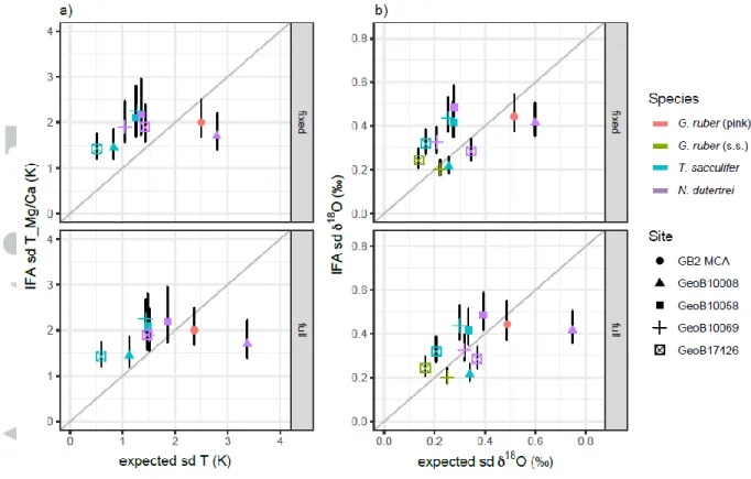
As a first test, we compare the observed single specimen variability to the predicted variability derived from analyzing the seasonal and interannual SST and ¹⁸Osw (predicted from salinity) variations at a fixed depth level (Figure 7, top row). We choose the mean depth level of their assumed habitat range (G. ruber, 25 m; T. sacculifer, 35 m; N. dutertrei, 100 m; Figure 2) but confirmed that the results are stable when varying this assumption.

The seasonal range in SST off Indonesia and in the WPWP is much lower than in the GoM (<4°C vs.

~7°C), but this is not always reflected in the spread in IF Mg/Ca and ¹⁸O. For sites in the WPWP and off Indonesia with an expected variability below sd = 2 °C, the observed variability from TMg/Ca is

above the expected variability (Figure 7). This behavior is largely mirrored for the observed IF ¹⁸O, showing that it is not a measurement or proxy artefact. In contrast, G. ruber in the GoM (GB2-MCA) and especially N. dutertrei at GeoB 10008-4 in the Northern Mentawai Basin show less reconstructed than predicted variability, both for TMg/Ca and ¹⁸O. The range for N. dutertrei at GeoB 10008-4 of the reconstructed spread (around 1°C sd T_Mg/Ca, 0.3‰ sd ¹⁸O) is much lower than the range of the predicted spread in seasonal and interannual temperatures (around 3°C sd T_Mg/Ca, 0.5‰ sd ¹⁸O) (Figures 1, 7). Thermocline conditions vary significantly throughout the year at the location of GeoB 10008-4, but a sediment trap study from off Java showed a clear seasonal flux for N. dutertrei (Mohtadi et al., 2009). This may explain why the analyzed variability in N. dutertrei is smaller than the expected variability, i.e. when the flux is concentrated to a short period of the year the expected variability will be skewed towards this time period and be less than the variability for a full year. This shows that the interpretation of thermocline-dwellers for IFA may be more complicated when the variability in the conditions becomes so large that the foraminifera restrict their habitat in which they live.

As there might also be variations in the depth habitat and thus the recorded water temperature from one foraminifer to the next, we also compared our reconstructed variability to the predicted variability derived from integrating the variability over the habitat range instead of a fixed average depth (G. ruber (s.s.) and G. ruber (pink) at 0-50 m, T. sacculifer at 20-70 m and N. dutertrei at 80-120 m). However, the results (Figure 7, lower panel) are largely unchanged.

Given our evidence that seawater temperature variability is the dominating factor for the single specimen variability, the likely explanation for our findings are site-specific seasonal and depth habitat changes. The single specimen variability can be reduced compared to the seasonal variability by only integrating one specific season, or enhanced compared to the variability at one single depth level by integrating across depth. In our results (Figure 7), the range of the recorded variations for Mg/Ca as well as for δ¹⁸O is smaller than the range of the expected variations from the oceanographic data suggesting that there is a preference of the species towards keeping their conditions constant (Mix et al., 1987) and thus to underestimate the true change in variability. The effect is likely stronger when the variability is large, such as in the thermocline of site GeoB 10008-4 where the largest mismatch between data and proxy (N. dutertrei) is observed (Figure 7).

Indeed, it is well known that planktic foraminifera have seasonal preferences and also migrate vertically during their lifecycle, recording the signal of the water depth in which they calcify throughout their habitat range (Fairbanks et al., 1982; Elderfield & Ganssen, 2000; Anand et al., 2003; Mohtadi et al., 2009; Jonkers & Kučera, 2015). Accordingly, the characteristics of different

water depths and seasons control the signal that is reflected by the shell chemistry and will thus modulate the recorded spread in IF Mg/Ca and ¹⁸O.

A previous example of how site-specific conditions may affect IFA variability was shown in a study from the Mediterranean Sea, which is characterized by a large salinity gradient. It was concluded that the spread in laser ablation-based Mg/Ca and ¹⁸O on single specimens of G. ruber was similar to the seasonal cycle (Wit et al., 2010). However, the lack of a relationship between Mg/Ca and ¹⁸O suggested that an additional impact of (seasonal) changes in salinity and the carbonate ion concentration might have affected the proxy signals and led to a differing impact of salinity on Mg/Ca and ¹⁸O (Wit et al., 2010). Additionally, when seasonal changes in SST are high as in the Mediterranean Sea, the seasonal flux of foraminifera may become more concentrated over a shorter time period also affecting the spread in IF geochemistry (Jonkers & Kučera, 2015).

4.6 Implications for paleoceanographic reconstructions

We have demonstrated a strong relationship between the single specimen variability in Mg/Ca and

¹⁸O. The consistency of the ratio of variability with the standard temperature calibration as well as the relationship between the variability of both proxies across individual sites demonstrates that single specimen variability is dominated by seawater temperatures during calcification.

However, while consistent between both temperature proxies, the observed variability cannot be fully explained by simple predictions from oceanographic temperature and salinity data alone. For example, comparing the full seasonal and interannual SST variability at our sites with the single specimen variability of the surface dwellers showed only a weak relationship, suggesting an effect of ecology leading to site-specific seasonal and depth habitat changes. Where the oceanographic variability is the strongest, the IFA variability (e.g. N. dutertrei at GeoB 10008-4) is significantly less than expected, as N. dutertrei appears to concentrate its flux to minimize varying conditions. This finding also suggests that the general relationship between IFA and variability may be less robust for sites affected by strong oceanographic/climatic variability.

This has important implications for paleo-studies using the variability in IFA to reconstruct seasonality (Ganssen et al., 2011) and/or interannual variability like ENSO (Koutavas et al., 2006;

Leduc et al., 2009; Scroxton et al., 2011; Sadekov et al., 2013; Rustic et al., 2015). The flux of foraminifera to the sediment can strongly depend on the species-specific preference for certain conditions. A certain species will thrive at the time of year and water depth where it experiences

ideal conditions (Mix, 1987; Skinner & Elderfield, 2005; Jonkers & Kučera, 2017). If these conditions change through time, e.g. last glacial in comparison with today, the season and depth recorded by a species may be shifted and thus affect the recorded mean and variability (Fraile et al., 2009). Using the spread in IF Mg/Ca and ¹⁸O as indicator for past changes in climate conditions may therefore be biased by the ecology reacting to changes in the structure of the water column.

Simple models parametrizing the foraminiferal flux as a function of environmental parameters (Mix, 1987; Schmidt & Mulitza 2002; Roche et al., 2017; Dolman et al., 2018) might allow first order estimates of these ecological effects. Further, more complex ecosystem modelling that also includes the interaction of secondary parameters such as nutrients has the potential to provide indications on how seasonality and habitat depth change in a different climatic setting (Lombard et al., 2011;

Kretschmer et al., 2018). This would help in isolating the part of the signal in IFA which represents changes in interannual variability or changes due to a shift in seasonality and depth habitat migration. However, the predictive quality of such an approach should be tested first on core-top data with known oceanographic conditions, such as the dataset presented here, or by directly comparing the geochemistry of foraminiferal tests from depth-specific plankton tows with water analyses before using it to reconstruct past climate variability.

Conclusions

We present for the first time a combined approach of the analysis of Mg/Ca and ¹⁸O on single specimens of foraminifera to investigate if its variability is related to climatic conditions or affected by analytical biases, intrinsic variability or ecological changes. The mixed-layer species G. ruber (s.s.), G. ruber (pink), and T. sacculifer and the thermocline-dwelling N. dutertrei were selected from core tops with widely differing seasonalities from the Indo Pacific Warm Pool, seasonal upwelling off Indonesia, and the Gulf of Mexico where large seasonal variations occur.

Our results indicate that the variability in Mg/Ca and ¹⁸O is mainly driven by seawater temperature and less by ¹⁸Osw variations during calcification, which allows the use of single specimen variability to infer environmental changes experienced by foraminifera. The results show that there is not always a simple relationship between the strength of the seasonal cycle and the spread in IFA;

generally all species show more variability than expected, but when conditions become highly variable, like for N. dutertrei in the thermocline at GeoB 10008-4 the variability is less than expected.

It is likely that the spread is additionally modulated by variations in the habitat depth of the foraminifera and its seasonality. Accordingly, IFA may also contain information on how the

foraminifera respond to changing climate conditions by adapting their season and habitat depth occurrence to optimize their living conditions thus minimizing variability when living in a highly variable setting. Our results suggest that the classic interpretation of IFA would be prone to underestimating the true extent to variability changes.

Our results call for further single specimen studies on modern core-tops and depth-stratified plankton tows to cover a larger range of oceanographic conditions and to estimate how variability changes in the water column. This would allow better characterizing the IFA signal; on one hand as a direct proxy of seasonal and interannual climate variability, on the other hand as a tool to constrain past changes in habitat depth. This may additionally be improved by performing IFA on foraminifera from depth-stratified plankton tows that can directly be compared with the water mass characteristics at the sampled water depth. Such datasets would also provide an ideal test-bed for statistical and ecosystem model based approaches to predict the habitat of foraminifera, and thus to ultimately improve the interpretation of foraminiferal based paleoclimate records.

Acknowledgements

We thank Silvana Pape, Henning Kuhnert and Lisa Schönborn for laboratory assistance; Ed C.

Hathorne for FT discussions; Kaustubh Thirumalai and Terry Quinn for providing the GoM core top;

Andrew Dolman for discussions, and Stephen Barker (Editor) and two anonymous reviewers for their constructive reviews. In memory of Matthias Lange who constructed the Bremen Flow- Through device. This project was supported by the Initiative and Networking Fund of the Helmholtz Association Grant VG-NH900 and European Research Council (ERC) under the European Union’s Horizon 2020 research and innovation program (grant agreement no. 716092) and the German Ministry for Education and Research (grant 03G0228A). The GODAS data was provided by the NOAA/OAR/ESRL PSD, Boulder, Colorado, USA, from their Web site at https://www.esrl.noaa.gov/psd/. The complete dataset will be archived in Pangaea (www.pangaea.de).

References

Anand, P., Elderfield, H., & Conte, M. H. (2003). Calibration of Mg/Ca thermometry in planktonic foraminifera from a sediment trap time series. Paleoceanography, 18, 1050.

doi:10.1029/2002PA000846

Barker, S., Greaves, M., & Elderfield, H. (2003). A study of cleaning procedures used for foraminiferal Mg/Ca paleothermometry. Geochemistry, Geophysics, Geosystems, 4.

doi:10.1029/2003GC000559

Behringer, D. W., & Xue, Y. (2004). Evaluation of the global ocean data assimilation system at NCEP:

The Pacific Ocean. Eighth Symposium on Integrated Observing and Assimilation Systems for Atmosphere, Oceans, and Land Surface, AMS 84th Annual Meeting, Washington State Convention and Trade Center, Seattle, Washington, 11-15.

Bemis, B. E., Spero, H. J., Bijma, J., & Lea, D. W. (1998). Reevaluation of the oxygen isotopic

Composition of planktonic foraminifera: Experimental results and revised paleotemperature equations. Paleoceanography, 13, 150-160

Billups, K., & Spero, H. J. (1996). Reconstructing the stable isotope geochemistry and

paleotemperatures of the equatorial Atlantic during the last 150,000 years: Results from individual foraminifera. Paleoceanography, 11, 217-238

Bouvier-Soumagnac, Y., & Duplessy, J.-C. (1985). Carbon and oxygen isotopic composition of planktonic foraminifera from laboratory culture, plankton tows and recent sediment:

Implications for the reconstruction of paleoclimatic conditions and of the global carbon cycle. Journal of Foraminiferal Research, 15, 302-320

Brown, S. J., & Elderfield, H. (1996). Variations in Mg/Ca and Sr/Ca ratios of planktonic foraminifera caused by postdepositional dissolution: Evidence of shallow Mg‐dependant dissolution.

Paleoceanography, 11, 543-551. doi:10.1029/96PA01491

Brugger, R. M. (1969). A note on unbiased estimation of the standard deviation. The American Statistician, 23 (4), 32-32

De Nooijer, L. J., Hathorne, E. C., Reichart, G. J., Langer, G., & Bijma, J. (2014). Variability in calcitic Mg/Ca and Sr/Ca ratios in clones of the benthic foraminifer Ammonia tepida. Marine Micropaleontology, 107, 32-43

Dolman, A. M., & Laepple, T. (2018). Sedproxy: a forward model for sediment archived climate proxies. Climate of the Past, https://doi.org/10.5194/cp-14-1851-2018

Eggins, S. M., Sadekov, A., & De Deckker, P. (2004). Modulation and daily banding of Mg/Ca in Orbulina universa tests by symbiont photosynthesis and respiration: a complication for seawater thermometry? Earth and Planetary Science Letters, 225, 411-419

Elderfield, H., & Ganssen, G. (2000). Past temperature and ¹⁸O of surface ocean waters inferred from foraminiferal Mg/Ca ratios. Nature, 405, 442-445

Fairbanks, R. G., Sverdlove, M., Free, R., Wiebe, P. H., & Bé, A. W. H. (1982). Vertical distribution and isotopic fractionation on living planktonic foraminifera from the Panama Basin. Nature, 298, 841-844

Fraile, I., Schulz, M., Mulitza, S., Merkel, U., Prange, M., & Paul, A. (2009). Modeling the seasonal distribution of planktonic foraminifera during the Last Glacial Maximum. Paleoceanography, 24, PA2216. doi:10.1029/2008PA001686

Ganssen, G. M., Peeters, F. J. C., Metcalfe, B., Anand, P., Jung, S. J. A., Kroon, D., & Brummer, G.-J. A.

(2011). Quantifying sea surface temperature ranges of the Arabian Sea for the past 20 000 years. Climate of the Past, 7, 1337-1349. doi:10.5194/cp-7-1337-2011

Greaves, M., Caillon, N., Rebaubier, H., Bartoli, G., Bohaty, S., Cacho, I., et al. (2008). Interlaboratory comparison study of calibration standards for foraminiferal Mg/Ca thermometry.

Geochemistry, Geophysics, Geosystems, 9, Q08010. doi:10.1029/2008GC001974

Groeneveld, J., Nürnberg, D., Tiedemann, R., Reichart, G.-J., Steph, S., Reuning, et al. (2008).

Foraminiferal Mg/Ca increase in the Caribbean during the Pliocene: Western Atlantic Warm Pool formation, salinity influence, or diagenetic overprint? Geochemistry, Geophysics, Geosystems, 9-1, Q01P23. doi:10.1029/2006GC001564

Groeneveld, J., & Chiessi, C. M. (2011). Mg/Ca of Globorotalia inflata as a recorder of permanent thermocline temperatures in the South Atlantic. Paleoceanography, 26, PA2203.

doi:10.1029/2010PA001940.

Grossman, E. L., & Ku, T.-L (1986). Oxygen and carbon isotope fractionation in biogenic aragonite:

Temperature effects. Chemical Geology, 59, 59-74

Haarmann, T., Hathorne, E. C., Mohtadi, M., Groeneveld, J., Kölling, M., & Bickert, T. (2011). Mg/Ca ratios of single planktonic foraminifer shells and the potential to reconstruct the thermal seasonality of the water column. Paleoceanography, 26, PA3218. doi:10.1029/2010PA002091 Haley, B. A., & Klinkhammer, G. P. (2002). Development of a flowthrough system for cleaning and

dissolving foraminiferal tests. Chemical Geology, 185, 51–69

Hathorne, E. C., James, R. H., & Lampitt, R. S. (2009). Environmental versus biomineralization controls on the intratest variation in the trace element composition of the planktonic foraminifera G. inflata and G. scitula. Paleoceanography, 24, PA4204.

doi:10.1029/2009PA001742

Hebbeln, D., Jennerjahn, T., Mohtadi, M., Andruleit, H., Baumgart, A., Birkicht, M., et al. (2005).

Report and preliminary results of RV SONNE Cruise SO-184, PABESIA, Durban (South Africa) – Cilacap (Indonesia) – Darwin (Australia), July 8^th – September 13^th, 2005. Berichte aus dem Fachbereich Geowissenschaften der Universität Bremen, 246. 142 pp.

Hollstein, M., Mohtadi, M. Rosenthal, Y., Moffa Sanchez, P., Oppo, D., Martínez Méndez, G., et al.

(2017). Stable oxygen isotopes and Mg/Ca in planktic foraminifera from modern surface sediments of the Western Pacific Warm Pool: Implications for thermocline

reconstructions. Paleoceanography, 32. doi:10.1002/2017PA003122

Houston, R. M., Huber, B. T., & Spero, H. J. (1999). Size-related isotopic trends in some Maastrichtian planktic foraminifera: methodological comparisons, intraspecific variability, and evidence for photosymbiosis. Marine Micropaleontology, 36, 169-188

Jonkers, L., de Nooijer, L. J., Reichart, G.-J., Zahn, R., Brummer, & Brummer, G.-J. A. (2012).

Encrustration and trace element composition of Neogloboquadrina dutertrei assessed from single chamber analyses – implications for paleotemperature estimates. Biogeosciences, 9, 4851-4860. doi:10.5195/bg-9-4851-2012

Jonkers, L., & Kučera, M. (2015). Global analysis of seasonality in the shell flux of extant planktonic foraminifera. Biogeosciences, 12, 2207-2226. doi:10.5194/bg-12-2207-2015

Jonkers, L., & Kučera, M. (2017). Quantifying the effect of seasonal and vertical habitat tracking on planktonic foraminifera proxies. Climate of the Past, 13, 573-586. doi:10.5194/cp-13-573- 2017

Katz, M. E., Cramer, B. S., Franzese, A., Hönisch, B., Miller, K. G., Rosenthal, Y., et al. (2010).

Traditional and emerging geochemical proxies in foraminifera. Journal of Foraminiferal Research, 40, 165-192

Khider, D., Stott, L. D., Emile-Geay, J., Thunell, R., & Hammond, D. E. (2011). Assessing El Niño Southern Oscillation variability during the past millennium. Paleoceanography, 26, PA3222.

doi:10.1029/2011PA002139

Killingley, J. S., Johnson, R. F., & Berger, W. H. (1981). Oxygen and carbon isotopes of individual shells of planktonic foraminifera from Ontong-Java Plateau, equatorial Pacific. Palaeogeography, Palaeoclimatology, Palaeoecology, 33, 193-204

Klinkhammer, G. P., Haley, B. A., Mix, A. C., Benway, H. M., & Cheseby, M. (2004). Evaluation of automated flow-through time-resolved analysis of foraminifera for Mg/Ca

paleothermometry. Paleoceanography, 19, PA4030. doi:10.1029/2004PA001050 Klinkhammer, G. P., Mix, A. C., & Haley, B. A. (2009). Increased dissolved terrestrial input to the

coastal ocean during the deglaciation. Geochemistry, Geophysics, Geosystems, 10, Q03009.

doi:10.1029/2008GC002219

Kretschmer, K., Jonkers, L., Kučera, M., & Schulz, M. (2018). Modeling seasonal and vertical habitats of planktonic foraminifera on a global scale. Biogeosciences, 15, 4405-4429. doi:10.5194/bg- 2017-429

Koutavas, A., deMenocal, P. B., Olive, G. C., & Lynch-Stieglitz, J. (2006). Mid-Holocene El Niño- Southern Oscillation attenuation revealed by individual foraminifera in eastern tropical Pacific sediments. Geology, 34, 993-996. doi:10.1130/G22810A.1

Laepple, T., & Huybers, P. (2014). Ocean surface temperature variability: Large model-data

differences at decadal and longer periods. Proceedings of the National Academy of Sciences, 111, 16682-16687. doi:10.1073/pnas.1412077111

Lea, D. W. (2004). Elemental and isotopic proxies of past ocean temperatures. In: Elderfield, H., ed., The oceans and marine geochemistry: Treatise on Geochemistry, Vol. 6: Oxford, Elsevier- Pergamon, 365–390.

Leduc, G., Vidal, L., Cartapanis, O., & Bard. E. (2009). Modes of eastern equatorial Pacific thermocline variability: Implications for ENSO dynamics over the last glacial period. Paleoceanography, 24, PA3202. doi:10.1029/2008PA001701

LeGrande, A. N., & Schmidt, G. A. (2006). Global gridded data set of the oxygen isotopic composition in seawater. Geophysical Research Letters, 33, L12604.

doi:10.1029/2006GL026011

Locarnini, R. A., Mishonov, V., Antonov, J. I., Boyer, T. P., Garcia, H. E., Baranova, O. K., et al. (2013).

World Ocean Atlas 2013, Volume 1: Temperature. S. Levitus, Ed., A. Mishonov Technical Ed.;

NOAA Atlas NESDIS 73, 40 pp.

Lombard, F., Labeyrie, L., Michel, E., Bopp, L., Cortijo, E., Retailleau, S., et al. (2011).

Modelling planktic foraminifer growth and distribution using an ecophysiological multi- species approach. Biogeosciences, 8, 853-873. doi:10.5194/bg-8-853-2011

McKay, C. L., Groeneveld, J., Filipsson, H. L., Gallego-Torres, D., Whitehouse, M. J., Toyofuku, T., et al.

(2015). A comparison of benthic foraminiferal Mn/Ca and sedimentary Mn/Al as proxies of relative bottom-water oxygenation in the low-latitude NE Atlantic upwelling system. Biogeosciences, 12, 5415-5428. doi:10.5194/bg-12-5415-2015

Metcalfe, B., Feldmeijer, W., de Vringer-Picon, M., Brummer, G.-J. A., Peeters, F. J. C., & Ganssen, G. M. (2015). Late Pleistocene glacial-interglacial shell-size-isotope variability in planktonic foraminifera as a function of local hydrography. Biogeosciences, 12, 4781-4807.

doi:10.5194/bg-12-4781-2015

Mix, A. C. (1987). The oxygen-isotope record of glaciation. In: The Geology of North America. The Geological Society of America, Vol. K-3, Ch. 6, 111-135

Mohtadi, M., Steinke, S., Groeneveld, J., Fink, H. G., Rixen, T., Hebbeln, D., et al. (2009). Low-latitude control on seasonal and interannual changes in planktonic foraminiferal flux and shell geochemistry off South Java: A sediment trap study. Paleoceanography, 24, PA1201.

doi:10.1029/008PA001636

Mohtadi, M., Oppo, D. W., Lückge, A., DePol-Holz, R., Steinke, S., Groeneveld, J., et al. (2011).

Reconstructing the thermal structure of the upper ocean: Insights from planktic

foraminifera shell chemistry and alkenones in modern sediments of the tropical eastern Indian Ocean. Paleoceanography, 26, PA3219. doi:10.1029/2011PA002132

Mohtadi, M., Bergmann, F., Blanquera, R. V. C., Buleka, J., Carag, J. W. M., Carriére-Garwood, J., et al., (2013). Report and preliminary results of RV SONNE cruise SO-228, Kaohsiung-Townsville, 04.05.2013-23.06.2013, EISPAC, WESTWIND, SIODP. Berichte aus dem Fachbereich

Geowissenschaften der Universität Bremen, 295, 113 pp.

Morard, R., Reinelt, M., Chiessi, C. M., Groeneveld, J., & Kucera, M. (2016) Tracing shifts of oceanic fronts using the cryptic diversity of the planktonic foraminifera Globorotalia inflata, Paleoceanography, 31, doi:10.1002/2016PA002977

Morimoto, M., Abe, O., Kayanne, H., Kurita, N., Matsumoto, E., & Yoshida, N. (2002). Salinity records for the 1997-98 El Niño from Western Pacific corals. Geophysical Research Letters, 29, 1540.

doi:10.1029/2001GL013521

Nürnberg, D. (2000). Taking the temperature of past ocean surfaces. Science, 289, 5485-5486 Petchey, F., & Ulm, S. (2012). Marine reservoir variation in the Bismarck region: An evaluation of

Spatial and temporal change in R and R over the last 3000 years. Radiocarbon, 54-1, 45-58 Poore, R. Z., Tedesco, K. A., & Spear, J. W. (2013). Seasonal flux and assemblage composition of

planktic foraminifers from a sediment-trap study in the northern Gulf of Mexico. Journal of Coastal Research, 63, 6-19

Regenberg, M., Nürnberg, D., Steph, S., Groeneveld, J., Garbe-Schönberg, D., Tiedemann, R., et al., (2006). Assessing the effect of dissolution on planktonic foraminiferal Mg/Ca ratios: Evidence from Caribbean core tops. Geochemistry, Geophysics, Geosystems, 7, Q07P15.

doi:10.1029/2005GC001019

Regenberg, M., Steph, S., Nürnberg, D., Tiedemann, R., & Garbe-Schönberg, D. (2009). Calibrating Mg/Ca ratios of multiple foraminiferal species with ¹⁸O-calcification temperatures:

Paleothermometry for the upper water column. Earth and Planetary Science Letters, 278,

324-336

Roche, D. M., Waelbroeck, C., Metcalfe, B., & Caley, T. (2018). FAME (v1.0): A simple module to simulate the effect of planktonic foraminifer species-specific habitat on their oxygen isotopic content. Geoscience Model Development, 11, 3587-3603.

https://doi.org/10.5194/gmd-11-3587-2018

Rosenthal, Y., Lohmann, G. P., Lohmann, K. C., & Sherrell, R. M. (2000). Incorporation and

Preservation of Mg in Gs. sacculifer: Implications for reconstructing sea surface temperatures and the oxygen isotopic composition of seawater. Paleoceanography, 15, 135-145

Rosenthal, Y., Perron-Cashman, S., Lear, C. H., Bard, E., Barker, S., Billups, K., et al. (2004).

Interlaboratory comparison study of Mg/Ca and Sr/Ca measurements in planktonic foraminifera for paleoceanographic research. Geochemistry, Geophysics, Geosystems, 5, Q04D09. doi:10.1029/2003GC000650

Rustic, G. T., Koutavas, A., Marchitto, T. M., & Linsley, B. K. (2015). Dynamical excitation of the tropical Pacific Ocean and ENSO variability by Little Ice Age cooling. Science, 350, 1537-1541, doi: 10.1126/science.aac9937

Sadekov, A., Eggins, S. M., De Deckker, P., & Kroon, D. (2008). Uncertainties in seawater

thermometry deriving from intratest and intertest Mg/Ca variability in Globigerinoides ruber.

Paleoceanography, 23, PA1215

Sadekov, A. Y., Ganeshram, R., Pichevin, L., Berdin, R., McClymont, E., Elderfield, H., et al. (2013).

Palaeoclimate reconstructions reveal a strong link between El Niño-Southern Oscillation and tropical Pacific mean state. Nature Communications, 4. doi:10.1038/ncomms3692

Sadekov, A. Y., Darling, K. F., Ishimura, T., Wade, C. M., Kimoto, K., Singh, A. D., et al. (2016).

Geochemical imprints of genotypic variants of Globigerina bulloides in the Arabian Sea.