FESOM-C: coastal dynamics on hybrid unstructured meshes
Alexey Androsov
AWI, IO, Vera Fofonova
AWI, Ivan Kuznetsov
HZG, Sergey Danilov
AWI, IAP, J, Natalja Rakowsky
AWI, Sven Harig
AWI, and Karen Helen Wiltshire
AWIAWIAlfred Wegener Institute for Polar and Marine Research, Bremerhaven, Germany
HZGInstitute of Coastal Research, Helmholtz-Zentrum Geesthacht, Geesthacht, Germany
IOShirshov Institute of Oceanology, Moscow, Russia
IAPA. M. Obukhov Institute of Atmospheric Physics, Moscow, Russia
JJacobs University, Bremen, Germany
Correspondence to:Alexey Androsov (alexey.androsov@awi.de)
Abstract.We describe FESOM-C, the coastal branch of the Finite-volumE Sea ice – Ocean Model (FESOM2), which shares with FESOM2 many numerical aspects, in particular, its finite-volume cell-vertex discretization. Its dynamical core differs by the implementation of time stepping, the use of terrain-following vertical coordinate and formulation for hybrid meshes composed of triangles and quads. The first two distinctions were critical for coding FESOM-C as an independent branch. The hybrid mesh capability improves numerical efficiency, since quadrilateral cells have fewer edges than triangular cells. They do 5
not suffer from spurious inertial modes of the triangular cell-vertex discretization and need less dissipation. The hybrid mesh capability allows one to use quasi-quadrilateral unstructured meshes, with triangular cells included only to join quadrilateral patches of differt resolution or instead of strongly deformed quadrilateral cells. The description of the model numerical part is complemented by test cases illustrating the model performance.
1 Introduction 10
Many practical problems in oceanography require regional focus on coastal dynamics. Although global ocean circulation models formulated on unstructured meshes may in principle provide local refinement, such models are as a rule based on assumptions that are not necessarily valid in coastal areas. The limitations on dynamics coming from the need to resolve thin layers, maintain stability for sea surface elevations comparable to water layer thickness or simulate the processes of wetting and drying make numerical approaches traditionally used in coastal models different from those used in large-scale models. For this 15
reason, combining a coastal and large-scale functionality in a single unstructured-mesh model, although possible, would still imply a combination of different algorithms and physical parameterizations. Furthermore, on unstructured meshes, numerical stability of open boundaries, needed in regional configurations, sometimes requires to mask certain terms in motion equations close to open boundaries. This would be an unnecessary complication for a large-scale unstructured-mesh model which is as a rule global.
20
The main goal of the development described in this paper was to design a tool, dubbed FESOM-C that is close to FESOM2 (Danilov et al., 2017) in its basic principles, but can be used as a coastal model. Its routines handling the mesh infrastructure are derived from FESOM2. However, the time stepping, vertical discretization, and particular algorithms, detailed below,
are different. FESOM-C relies on terrain-following vertical coordinate (vs. the Arbitrary Lagrangian Eulerian (ALE) vertical coordinate of FESOM2), but does a step further with respect to the mesh structure. It is designed to work on hybrid meshes composed of triangles and quads. Some decisions, such as for example, the lack of the ALE at the present stage, are only motivated by the desire to keep the code as simple as possible through the initial phase of its development and maintenance.
The code is based on the cell-vertex finite-volume discretization, same as FESOM2 (Danilov et al., 2017) and FVCOM (Chen 5
et al., 2003). It places scalar quantities at mesh vertices and the horizontal velocities at cell centroids.
Our special focus is on using hybrid meshes. In essence, the capability of hybrid meshes is build in finite-volume method.
Indeed, computations of fluxes are commonly implemented as cycles over edges, and the edge-based infrastructure is immune to the polygonal type of mesh cells. However, because of staggering, it is still convenient to keep some computations on cells, which then depend on the cell type. Furthermore, high-order transport algorithms might be sensitive to the cell geometry 10
too. We limit the allowed polygons to triangles and quads. Although there is no principal limitation on the polygon type, triangles and quads are versatile enough in practice for the cell-vertex discretization. Our motivation of using quads is two-fold (Danilov and Androsov, 2015). First, quadrilateral meshes have 1.5 times fewer edges than triangular meshes, which speeds up computations because cycles over edges become shorter. The second reason is the intrinsic problem of the triangular cell- vertex discretization — the presence of spurious inertial modes (see, e.g., Le Roux (2012)) and decoupling between the nearest 15
horizontal velocities. Although both can be controlled by lateral viscosity, the control leads to higher viscous dissipation over the triangular portions of the mesh. The hybrid meshes can be designed so that triangular cells are included only to optimally match the resolution or even absent altogether. For example, FESOM-C can be run on curvilinear meshes combining smooth changes in the shape of quadrilateral cells with smoothly approximated coastlines. One can also think of meshes where triangular patches are only used to provide transitions between quadrilateral parts of different resolution, implementing an 20
effective nesting approach.
Many unstructured-mesh coastal ocean models were proposed recently (e.g., Casulli and Walters, 2000; Chen et al., 2003;
Fringer et al., 2006; Zhang and Baptista, 2008; Zhang et al., 2016). It will take some time for FESOM-C to catch them up as concerns functionality. The decision on the development of FESOM-C was largely motiated by the desire to fit in the existing modeling infrastructure (mesh design, analysis tools, input-output organization), and not by any deficiency ofexisting models.
25
The real work load was substantially reduced through the use or modification of the existing FESOM2 routines.
We formulate the main equations and their discretization in the three following sections. Section 5 presents results of test simulations, followed by discussion and conclusions.
2 Model formulation
2.1 The Governing Equations 30
We solve standard primitive equations in the Boussinesq, hydrostatic and traditional approximations. The solution is sought in the domainQb=Q×[0, tf], wheretf is the time interval. The boundary ∂Qof domainQis formed by the free water surface, the bottom, and lateral boundaries, composed of the solid part∂Q1and the open boundary∂Q2,Q={x, y, z;x, y∈
Ω,−h(x, y)≤z < ζ(x, y, t)},0≤t≤tf. Hereζis the surface elevation andhthe bottom topography. We seek the vector of unknownq= (u, w, ζ, T, S), whereu= (u, v)is the horizontal velocity,wthe vertical velocity,T the potential temperature andSthe salinity,
∂u
∂t + ∂
∂xi
(uui) + ∂
∂z(uw) + 1
ρ0∇p+fk×u= ∂
∂zϑ∂u
∂z+∇ ·(K∇)u, (1)
5
∇ ·u+ ∂
∂zw= 0, (2)
∂p
∂z=−gρ, (3)
∂Θj
∂t +ui
∂Θj
∂xi
+w∂Θj
∂z = ∂
∂zϑΘ
∂Θj
∂z +∇(KΘ∇)Θj, (4)
10
herei= 1,2,x1=x,x2=y,u1=u,u2=v, and summation is implied over the repeating indicesi;pis the pressure;j= 1,2 withΘ1=T,Θ2=Sthe potential temperature and salinity respectively. The seawater density is determined by the equation of stateρ=ρ(T, S, p),ρ0 is the reference density;f is the Coriolis parameter;kis the vertical unit vector; ϑandKare the coefficients of vertical and horizontal turbulent momentum exchange, respectively;ϑΘ andKΘ are the respective diffusion coefficients andgis the acceleration due to gravity.
15
Writing
ρ(x, y, z, t) =ρ0+ρ0(x, y, z, t), (5)
whereρ0density fluctuation, we obtain, integrating Eq.(3),
p−patm= Zζ z
ρgdz=gρ0(ζ−z) +g Zζ z
ρ0dz,
wherepatmis the atmospheric pressure. The horizontal pressure gradient is expressed then as the sum of barotropic, baroclinic 20
and atmospheric pressure gradients:
ρ−10 ∇p=g∇ζ+gρ−10 ∇I+ρ−10 ∇patm, I= Zζ z
ρ0dz. (6)
Note that horizontal derivatives here are taken at fixedz.
2.2 Turbulent closures
The default scheme to compute the vertical viscosity and diffusivity in the system of equations (1-4) is based on the Prandtl- Kolmogorov hypothesis of incomplete similarity. According to it, the turbulent kinetic energyb, the coefficient of turbulent mixingϑand dissipation of turbulent energyεare connected asϑ=l√
b, wherel is the scale of turbulence,ϑΘ=cρϑ,ε= cεb2/ϑ;cε= 0.046(Cebeci and Smith, 1974). Prandtl’s numbercρis commonly chosen as 0.1 and sets the dependence between 5
the coefficients of turbulent diffusion and viscosity. The equation describing the balance of turbulent kinetic energy is obtained by parameterizing the energy production and dissipation in the equation for turbulent kinetic energybas
∂b
∂t−ϑ(|uz|2+cρgρ−01∂ρ
∂z) +cεb2/ϑ=αb
∂
∂zϑ∂b
∂z, (7)
with the boundary conditions b|h=B1|ϑ|2, ϑbz|ζ=Hγζu3∗ζ, 10
whereH=h+ζis the full water depth,αb= 0.73, B1= 16.6, γζ = 0.4·10−3;u∗ζ= (ρ/ρa)1/2u∗is the dynamical velocity in water near the surface,ρathe air density,u∗the dynamic velocity of water on the interface between air and water.
Equation (7) is solved iteratively in the vertical direction for the nonlinear dissipative term. It is written as cεb2/ϑ= (2bν+1bν−(b2)ν)/ϑν,
whereνis the index of iterations, which are repeated untill convergence.
15
To determine the turbulence scalelin the presence of surface and bottom boundary layers we use the Montgomery formula (Reid , 1957)
l= κ HZhZζ,
whereZh=z+h+zh,Zζ=−z+ζ+zζ,κ'0.4is the von Kármán constant,zthe layer depth andzh, zζare the roughness parameters for the bottom and free surface respectively. To remove turbulent mixing in layers that are distant from interfaces 20
we modify the Montgomery formula by introducing the cut-off functionZ0= 1−β1H−2ZhZζ,0≤β1≤4(Voltzinger, 1985) l= κ
HZhZζZ0.
In addition to the default scheme, one may select a scheme provided by the General Ocean Turbulence Model (GOTM) (Burchard et al., 1999) implemented into the FESOM-C code for computing vertical eddy viscosity and diffusion for mo- mentum and tracer equations. GOTM includes large number of well-tested turbulence models with at least one member of 25
every relevant model family (empirical models, energy models, two-equation models, Algebraic Stress Models, K-profile pa- rameterisations, etc) and treats every single water column independently. Essential part of GOTM is occupied by one-point second-order schemes (Umlauf and Burchard, 2005; Umlauf et al., 2005, 2007).
2.3 Bottom friction parametrization
The model uses either a constant bottom friction coefficientCd, or it is computed through the specified bottom roughness heightzh. The first option is preferable if the vertical resolution everywhere in the domain does not resolve the logarithmic layer or when the vertically averaged equations are solved. In the second option the bottom friction coefficient is computed according to Blumberg and Mellor (1987) and has the following form
5
Cd= (ln(H/zh)/κ)2.
It is also possible to prescribeCdorzhas a function of horizontal coordinate at the initialization step.
2.4 Boundary conditions
The boundary conditions for the dynamical equations (1-2) are those of no-slip on the solid boundary∂Q1, u|∂Q1= 0.
10
As is well known, formultion of open boundary conditions faces difficulties. They are related to either the lack or incom- pleteness of information demanded by the theory, for example, on velocity components at the open boundary. Furthermore, whatever the external information, it may contradict to the solution inside the computational domain, leading to instabilities which are frequently expressed as small-scale vortex structures forming near the open boundary. The procedure reconciling the external information with the solution inside the domain becomes of paramount importance. We use two approaches. The first 15
one is to use a function whereby advection and horizontal diffusion are smoothly tapered to zero in the close vicinity of open boundary∂Q2. Such tapering makes the equations hyperbolic at the open boundary, so that the formulation of one condition (for example, for the elevation,ζ|∂Q2=ζΓ) is possible (Androsov et al., 1995).
The other approach is to adapt the external information. It is applied to scalar fields and will be explained further.
Note that despite simplifications, barotropic and baroclinic perturbations still may disagree at the open boundary, leading to 20
instabilities in its vicinity. In this case an additional buffer zone is introduced with locally increased horizontal diffusion and bottom friction.
Dynamic boundary conditions on the top and bottom specify the momentum fluxes entering the ocean. Neglecting the contributions from horizontal viscosities, we write
ϑ∂u
∂z|ζ=τζ/ρ0, ϑ∂u
∂z|−h=τh/ρ0=Cd|uh|uh. 25
The first of them sets the surface momentum flux to the wind stress at the surface (τζ), and the second one, sets the bottom momentum flux to the frictional flux at the bottom (τh), withuhthe bottom velocity.
Now we turn to the boundary conditions for the scalar quantities obeying equation (4). This is a three-dimensional parabolic equation and the boundary conditions are determined by its leading (diffusive) terms. We impose the no-flux condition on the solid boundary∂Q1
30
∂Θj
∂n |∂Q1= 0.
The conditions at the open boundary∂Q2are given for outflow and inflow as Barnier et al. (1995); Marchesiello et al. (2001) Θt+aΘx+bΘy=−1
τ(Θ−ΘΓ),
whereΘΓis the given field value, usually a climatological one or relying on data from a global numerical model or observations.
If the phase velocity componentsa=−ΘtΘx/G,b=−ΘtΘy/GandG= [(∂Θ/∂x)2+ (∂Θ/∂y)2]−1, Raymond and Kuo (1984) show thatΘpropagates out of the domain, thenτ=τ0. If it propagates into the domain, thenaandbare set to zero and 5
τ=τΓ, withτΓτ0. The parameterτis determined experimentally and commonly is from hours to days. In the FESOM-C such an adaptive boundary condition is routinely applied for temperature and salinity, yet it can also be used for any components of solution.
The vertical boundary condition for the tracer equation (4) is that of zero flux atz=−h(the bottom is insulated) ϑΘ
∂Θj
∂n |−h= 0, (8)
10
where the derivative is in the direction normal to the surface (i= 1,2,Θ1=T,Θ2=S) and we neglect the contributions from horizontal diffusion. At the surface the fluxes are due to the interaction with the atmosphere,
ϑΘ
∂T
∂z|ζ= ˆQ(x, y, t)/ρ0cp, (9)
ϑΘ
∂S
∂z|ζ=WsSw/ρ0, (10)
15
whereQˆ is the heat flux,cρ the specific heat of sea water,Ws=E−P is the evaporation minus precipitation rates, andSw
is the salinity of added water. In most casesSw= 0. In the presence of rivers, their discharge is added either as a prescribed inflow at the open boundary in the river mouth, or as volume sources of mass, heat and momentum distributed in the vicinity of open boundary. In the first case it might create an initial shock in elevation, so the second method is safer.
3 Temporal discretization 20
As is common in coastal models, we split the fast and slow motions into, respectively, barotropic and baroclinic subsystems (Lazure and Dumas, 2008; Higdon, 2008; Gadd, 1978; Blumberg and Mellor, 1987; Deleersnijder and Roland , 1993). The reason for this splitting is that surface gravity waves (external mode) are fast and impose severe limitations on the time step, whereas the internal dynamics can be computed with a much larger time step. The time step for the external modeτ2D is limited by the speed of surface gravity waves, and that for the internal mode,τ3D, by the speed of internal waves or advection.
25
The ratioMt=τ3D/τ2Ddepends on applications, but is commonly between 10 and 30. In practice, additional limitation are due to vertical advection, or wetting and drying processes. We will further use the indiceskandnto enumerate the internal and external time steps respectively.
The numerical algorithm passes through several stages. On the first stage, based on the current temperature and salinity fields (time stepk) the pressure is computed from hydrostatic equilibrium equation (6) and then used to compute the baroclinic 30
pressure gradientρ−10 ∇p=g∇ζk+gρ−10 ∇Ik+ρ−10 ∇patm. We use an asynchronous time stepping, assuming that integration of temperature and salinity is half-step shifted with respect to momentum. The indexkonIimplies that it is centered between kandk+ 1of momentum integration. The elevation in the expression above is taken at time stepk, which makes the entire estimate for∇ponly first-order accurate with respect to time.
At the second stage, the predictor values of the three-dimensional horizontal velocity are determined as 5
˜
uk+1−uk=τ3D(−fk×u− ∇ ·uu+∇ ·(K∇u))AB3−τ3Dρ−01∇p+τ3D∂zϑ∂zu˜k+1−τ3D∂z(wu)AB3,
hereKis the coefficient of horizontal viscosity, andAB3implies the Adams–Bashforth third-order estimate. The horizontal viscosity operator can be made biharmonic or replaced with filtering as discussed in the next chapter.
To carry out mode splitting, we write the horizontal velocity as the sum of the vertically averaged oneu¯ and the deviation thereof (pulsation)u0:
10
u= ¯u+u0, u¯= 1 H
Zζ
−h
udz, Zζ
−h
u0= 0.
By integrating the system (1)-(3) vertically between the bottom and surface, with regard for the kinematic boundary conditions
∂tζτ2D+u∇ζ=won the surface and−u∇h=wat the bottom and time discretization, we get (ζn+1−ζn) +τ2D∇(Hu)¯ AB3= 0,
15
¯
un+1−u¯n=τ2D(−fk×u¯− ∇ ·u¯¯u+∇ ·(K∇¯u))AB3−τ2D(g∇ζ)AM4+τ2D(τζ/ρ0−τh)−τ2DR3D0 −τ2Dgρ−10 ∇I¯k. Here a specific version ofAB3is used, ¯uAB3= (3/2 +β)¯uk−(1/2 + 2β)¯uk−1+β¯uk−2, withβ= 0.281105for stability reasons (Shchepetkin and McWilliams, 2005);AM4implies the Adams–Multon estimateζAM4=δζn+1+(1−δ−γ−)ζn+ γζn−1+ζn−2, taken withδ= 0.614,γ= 0.088,= 0.013(Shchepetkin and McWilliams, 2005). In the equations aboveτs, τbare the surface (wind) and bottom stresses respectively,∇I¯is the vertically integrated gradient of baroclinic pressure. The 20
termR03Dcontains momentum advection and horizontal dissipation of the pulsation velocity integrated vertically
R03D= 1 Hk[
Zζ
−h
∇ ·u0u0− Zζ
−h
∇ ·(K∇u0)]k.
In this expressionHkis the total fluid depth at time stepk,Hk=h+ζk. This term is computed only on the baroclinic time step and kept constant through the integration of the internal mode.
The bottom friction is taken as 25
τh=Cd|u¯|n(¯un+1−u¯n)/Hn+1+Cd|u˜h|k+1u˜k+1h /Hn+1.
The first part of bottom friction is needed to increase stability, while the second part estimates the correct friction, withu˜k+1h the horizontal velocity vector in the bottom cell on the predictor time step.
The system of the vertically averaged equations is stepped explicitly (except for the bottom friction) throughMttime steps of durationτ2D(indexn), to ’catch up’ thek+ 1baroclinic time step. The update of elevation is made first, followed by the update of vertically integrated momentum equations.
At the "corrector" step, the 3D velocities are corrected to the surface elevation atk+ 1 uk+1= 4ki
4k+1i
˜
uk+1+ (¯uk+1−u¯P), 5
withu¯P =Hk+11 Pζ
−h(˜uk+14ki),i is the vertical index. Here 4ki,4k+1i are the thickness of thei-th layer calculated on respective baroclinic time steps. The layer thickness is4ki =4iHk/H. This correction removes the barotropic component of the predicted velocity and combines the result with the computed barotropic velocity. We will suppress the layer indexiwhere it is unambiguous.
The final step in the dynamical part calculates the transformed vertical velocitywk+1from 3D continuity equation (2). It is 10
used in the next predictor step. Note that in the predictor step the computations of vertical viscosity are implicit.
New horizontal velocities, the so-called "filtered" ones, are used for avection of tracer. They are given by the sum of the
"filtered" depth-mean and the baroclinic part of the "predicted" velocities (Deleersnijder, 1993), uk+1F = 4ki
4k+1i
u˜k+1+ (¯uF−u¯P), withu¯F=M 1
tHk+1
Pn=Mt
n=1 (¯unHn). The procedure of "filtering" removes possible high-frequency component in the barotropic 15
velocity. It also improves accuracy for it in essence works toward centering the contribution of the elevation gradient. Once the filtered velocity is computed, the vertical velocity is updated to match it.
Then, the equation for temperature will be computed in the conservation form:
4k+1Tk+1=4kTk−τ3D[∇ ·(uk+1F 4kT∗) +wF tTt∗−wF bTb∗] +D+τ3DR+τ3DC,
whereDcombines the terms related to diffusion,wF t, wF b,Tt, Tbare the vertical transport velocity and temperature on top 20
and bottom of the layer,T∗ will be computed trough second-order Adams–Bashforth (AB) time stepping method.Ris the boundary termal flux (either from surface, or due to river discharge). The last term in the equation above is
C=T∂4i
∂t =−T(∇(4iuk+1F ) +∂z(4iwFk+1)).
Its two constituents combine to zero because of continuity. Keeping this term makes sense if computation of advection are split into horizontal and vertical substeps. The salinity is treated similarly.
25
In simulations of coastal dynamics it is often necessary to simulate flooding and drying events. Explicit time stepping methods of solving the external mode are well suited for this (Luyten et al., 1999; Blumberg and Mellor, 1987; Shchepetkin and McWilliams, 2005). The algorithm to account for wetting and drying will be presented in the next section. We only note that computations are performed on each time step of the external mode.
4 Spatial discretization
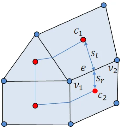
In the finite-volume method, the governing equations are integrated over control volumes and the divergence terms, by virtue of the Gauss theorem, are expressed as the sums of respective fluxes through the boundaries of control volumes. For the cell- vertex discretization the scalar control volumes are formed by connecting cell centroids with the centers of edges, which gives the so-called median-dual control volumes around mesh vertices. The vector control volumes are the mesh cells (triangles or 5
quads) themselves, as schematically shown in Fig. 1.
The basic structure to describe the mesh is the array of edges given by their verticesv1andv2, and the array of two pointers c1andc2to the cells on the left and on the right of the edge. There is no difference between triangles, quads or hybrid meshes in the cycles which assemble fluxes. Quads and triangles are described through four indices to vertices forming them; in the case of triangles the fourth index equals the first one. The treatment of triangles and quads differs slightly in computations of 10
gradients as detailed below. We will use symbolic notation:e(c)for the list of edges forming cellc,e(v)for the list of edges connected to vertexv,v(c)for the list of vertices defining cell of elementc.
In the vertical direction we introduce aσ-coordinate (Phillips, 1957) σ=z+h
h+ζ, 1≤σ≤0.
The lower and upper horizontal faces correspond to the planesσ= 0andσ= 1respectively. The vertical grid spacing is 15
defined by the selected set ofσi. The spacing ofσiis horizontally uniform in present implementation (but it can be varying) and can be selected as equidistant or based on a parobolic function with high vertical resolution near surface and bottom in the vertical,
σi=−( i−1 N−1)%+ 1,
whereN is the number of vertical layers. Here%= 1(2)gives the uniform (parabolic) distribution of vertical layers. One 20
more possibility to use refined resolution near bottom or surface is implemented through the formula by Burchard and Bolding (2002):
σi=tanh[(Lh+Lζ)(N(N−−1)i)−Lh] + tanhLh
tanhLh+ tanhLζ −1,
whereLhandLζ are the number of layers near bottom and surface respectively.
The vertical grid spacing is recalculated on each baroclinic time step for the vertices, whereζis defined. It is interpolated 25
from vertices to cells and to edges. The vector of horizontal velocity and tracers are located in the middle of vertical layers (indexi+ 1/2), but the vertical velocity is at full layers.
4.1 Divergence and gradients
Thedivergence operatoron scalar control volumes is computed as:
Z
v
∇(4u)dS= X
e=e(v)
[(4un`)l+ (4un`)r], 30
where the cycle is over edges containing vertexv, the indiceslandrimply that the estimates are made on the left and right segments of the control volume boundary attached to the center of edgee,nis the outer normal and`the length of the segment.
Vectorsslandsrconnecting the mid-point of edgeewith the elements on the left and on the right, we get(n`)l=k×sland similarly, but with the minus sign for the right element (kis a unit vertical vector). The mean cell values, for example layer thickness on the cell, can be defined as4c=P
v=v(c)4vwcv, wherewcv= 1/3 on triangles andwcv=Scv/Sc for quads 5
(Sc-cell area andScv-the part of it in the scalar control volume around vertex).
Gradients of scalarquantities are needed on cells, and are computed as:
Z
c
∇ζdS= X
e=e(c)
(n`ζ)e,
where summation is over the edges of cellc, the normal and length are related to the edges, andζis estimated as the mean over edge vertices.
10
Thegradients of velocitieson cells can be needed for computation of viscosity and momentum advection term. They are computed through the least squares fit based on the velocities on neighboring cells.
£= X
n=n(c)
(uc−un−(αx, αy)rcn)2= min.
Herercn= (xcn, ycn)is the vector connecting the center ofcto that of its neighborn. Their solution can be reformulated in terms of two sets of two matrix (computed once and stored)axcn= (xcnY2−ycnXY))/dandaycn= (ycnX2−xcnXY))/d, 15
acting on velocity differences and returning the derivatives. Hered=X2Y2−(XY)2,X2=P
n=n(c)x2cn,Y2=P
n=n(c)y2cn andXY =P
n=n(c)xcnycn. 4.2 Momentum advection
We implemented two options for horizontal momentum advection in the flux form. The first one is the linear reconstruction upwind, based on cell control volumes. The second one is central and is based on scalar control volumes, with subsequent 20
averaging to cells. In the upwind implementation we write Z
c
∇(u4u)dS= X
e=e(c)
(un`4u)e.
For edgee, linear velocity reconstructions on the elements on its both sides are estimated at the edge center. One of the cells isc, and letnbe its neighbor acrosse. The respective velocity estimates will be denoted asuceandune and upwind will be written in form2u=uce(1 + sgn(un)) +une(1−sgn(un)), whereun=n((uce+une))/2.
25
The other form is adapted from Danilov (2012). It provides additional smoothing for momentum advection by computing flux divergence for larger control volumes. In this case we first estimate the momentum flux term on scalar control volumes, Z
v
∇(u4u)dS= X
e=e(v)
[(un`4u)l+ (un`4u)r].
The notation here follows that for the divergence. No velocity reconstruction is involved. These estimates are then averaged to the centers of cells. In both variants of advection form the fluid thickness is estimated at cell centers.
30
4.3 Tracer advection
Horizontal advection and diffusion terms are discretized explicitly in time. Three advection schemes have been implemented.
The first two are based on linear reconstruction for control volume and are therefore second-order. The linear reconstruction upwind scheme and Miura scheme Miura (2007) differ in the implementation of time stepping. The first of them needs the Adams-Bashforth method to be the second-order with respect to time. The scheme by Miura reaches this by estimating the 5
tracer at a point displaced byuτ3D/2. In both cases a linear reconstruction of tracer field for each scalar control volume is performed,
ΘR(x, y) = Θ0(xv, yv) + Θx(x−xv) + Θy(y−yv),
whereΘ0is the tracer value at vertex,ΘxandΘyare the gradients averaged to vertex locations, andxv, yvthe coordinates of vertexv. The fluxes for scalar control volume faces associated to edgeeare computed as
10 X
e=e(v)
([(un`4ΘR)l+ (un`4ΘR)r]).
The estimate of tracer is made at the mid-points of the left and right segments, and at points displaced byuτ3D/2from them respectively.
The third approach used in the model is based on the gradient reconstruction. The idea of this approach is to estimate the tracer at mid-edge locations by a linear reconstruction using the combination of centered and upwind gradientsΘ±e = 15
Θvi±`e(∇Θ)±e/2,i= 1,2are the indices of edge vertices, and gradients are computed as (∇Θ)+e =2
3(∇Θ)c+1
3(∇Θ)u and (∇Θ)−e =2
3(∇Θ)c+1 3(∇Θ)d,
here, the upper indexcmeans centered estimates, andu,dimply the estimates on the up- and down- edge cells.
The advective flux of scalar quantityΘthrough the face of the scalar volume(Qe= [(un`4)l+ (un`4)r])associated with edgeewhich leaves the control volumeν1is
20
QeΘe=1
2Qe(Θ+e + Θ−e) +1
2(1−γ)|Qe|(Θ+e + Θ−e),
γis the parameter controlling the upwind dissipation. Takingγ= 0give the third-order upwind method whereasγ= 1gives the centered fourth-order estimate.
A quadratic upwind reconstruction is used in the vertical with the flux boundary conditions on surface (9) and (10) and zero flux at the bottom. Other options for horizontal and vertical advection, including limiters, will be introduced in future.
25
The advection schemes are coded so that their order can be reduced toward the first-order upwind for very thin water layer to increase stability in the presence of wetting and drying.
4.4 Viscosity and filtering
Consider the operator∇A∇u. Its computation follows the rule:
Z
c
∇A∇udS= X
e=e(c)
A`(n∇u)e
The estimate of velocity gradient on edgeeis symmetrized, following the standard practice, over the values on neighboring cells. The consequence of this symmetrization is that on regular meshes (formed of equilateral triangles or rectangular quads) 5
the information from the nearest neighbors will be lost. Any irregularity in velocity on the nearest cells will not be penalized.
Although unfavorable for both quads and triangles, it has further reaching implications for the latter: it cannot efficiently remove the decoupling between the nearest velocities which may occur for triangular cells. This fact is well known, and the modification of the scheme above that improves coupling between the nearest neighbors, consists in using the identity n=rcn/|rcn|+ (n−rcn/|rcn|),
10
wherercnis the vector connecting the centroid of cellscandn. The derivative in the direction ofrcnis just the difference between the neighboring velocities divided by the distance, which is explicitly used to correctn∇u. It is easy to show that on rectangular quads or equilateral triangles (nandrcnare collinear) the second term of the expression above will disappear. This is the harmonic discretization and a biharmonic version is obtained by applying the procedure twice.
A simpler algorithm is implemented to control grid-scale noise in the horizontal velocity. It consists in adding to the right 15
hand for the momentum equation (2D and 3D flow) a term coupling the nearest velocities, Fc=−(1
τf
)X
n(c)
(un−uc),
whereτf a time scale selected experimentally. On regular meshes this term is equivalent to the Laplacian operator. On general meshes it deviates from the Laplacian, yet after some trivial adjustments it warrants momentum conservation and energy dissipation.
20
4.5 Wetting and drying algorithm
For modeling wetting and drying we use the method proposed by Stelling and Duinmeijer (2003). The idea of this method is to accurately track the moving shoreline by employing the upwind water depth in the flux computations. The criterion for a vertex to be wet or dry is taken as:
wet, if Dwd=h+ζ+hl> Dmin
dry, if Dwd=h+ζ+hl≤Dmin, 25
whereDminis the critical depth andhlis the bathymetric land height. Each cell is treated as:
wet, if Dwd= minhv(c)+ maxζv(c)> Dmin
dry, if Dwd= minhv(c)+ maxζv(c)≤Dmin,
wherehvandζvare the depth and sea surface height at the verticesv(c)of the cellc. When a cell is treated as dry, the velocity at its center is set to zero and no volume flux passes through the boundaries of scalar control volumes inside this cell.
5 Numerical simulations
In this section we present the results of two model experiments. The first of them considers tidal circulation in the Sylt–Rømø Bight. This area has a complex morphometry with big zones of wetting/drying and large incoming tidal waves. In this case 5
our intention is to test functioning of meshes of various kind. The second experiment simulates a South-East part of the North Sea. For this area, annual simulation of barotropic-baroclinic dynamics with realistic boundary conditions on open and surface boundaries is carried out and compared to observations. We note that a large number of simpler experiments, including those where analytical solutions are known, were carried out in the course of model development, to test and tune the model accuracy and stability. Lessons learned from them where taken into account. We omit their discussion in favor of realistic simulations.
10
5.1 Sylt-Rømø experiment
To test the code sensitivity to the type of grid and grid quality we computed barotropic tidally driven circulation in the Sylt- Rømø Bight in the Wadden Sea.
It is a popular area for experiments and test cases (e.g. Lumborg and Pejrup, 2005; Ruiz-Villarreal et al., 2005; Burchard et al., 2008; Purkiani et al., 2014). The Sylt and Rømø islands are connected to the mainland by artificial dams, creating a 15
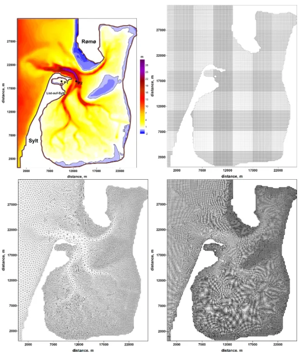
relatively small semi-enclosed bight with a circulation pattern well-known from observations and modeling (e.g. Becherer et al., 2011; Purkiani et al., 2014). It is a tidally energetic region with the water depth down to 30 m, characterized by wide intertidal flats and a rugged coastline. Water is exchanged with the open sea through a relatively narrow (up to 1.5 km wide) and deep (up to 30 m) tidal inlet Lister Dyb. The bathymetry data for the area was provided by H. Burchard and is presented in Fig 2.
20
We constructed three different meshes (Fig. 2) for our experiments. The first one is a nearly regular quadrilateral mesh, complemented by triangles that straighten the coastline (MESH-1). Its spatial resolution is 200 m. The second mesh is purely triangular (MESH-2) with resolution varying from∼820 to∼90 m. The third mesh was generated by the Gmsh mesh generator (Geuzaine and Remacle, 2009) and includes 34820 quads and 31 triangles with the minimum cell size of 30 m and maximum size of∼260 m (MESH-3). All meshes have 21 non-uniform sigma layers in the vertical direction (refined near the surface and 25
bottom). The wetting/drying option is turned on. We apply thek−turbulence closure model with transport equations for the turbulent kinetic energy and the turbulence dissipation rate using GOTM library. The second-moment closure is represented by algebraic relations suggested by Cheng et al. (2002). The experiment is forced by prescribing elevation due toM2tidal wave at the open boundary (western and northern boundaries of the domain).
Simulations on each mesh were continued until reaching the steady state in the tidal cycle ofM2wave. The last tidal period 30
was analyzed. The quasi-stationary behavior is established already on the second tidal period. The simulatedM2 wave is essentially nonlinear during the tidal cycle judged by the difference in amplitude of two tidal half-cycles.
Figure 3 shows the behavior of potential and kinetic energies in the entire domain, whereas the right panels show the energies computed over the areas deeper than 1 m. The results are sensitive to the meshes, which is explained further. The smallest tidal energy is simulated on the triangular mesh (MESH-2). The reason is that with the same value of the time scaleτf in the filter used by us in these simulations the effective viscous dissipation is much higher on a triangular mesh than on quadrilateral meshes of similar resolution. However, the solutions on quadrilateral meshes are different too, and this time the reason is the 5
difference in the details of representing very shallow areas on meshes of various resolution (MESH-3 is finer than MESH-1).
The difference between the simulations on two quadrilateral meshes is related to the potential energy and comes from the difference in the elevation simulated in the areas subject to wetting and drying. Note that the velocities and layer thickness are small in these areas, so the difference between kinetic energies between the left and right bottom panels of Fig. 3 is small.
The average currents, sea level and residual circulation simulated on MESH-1 are presented in Fig. 4. The results of this 10
experiment show good agreement with the previously published results of Ruiz-Villarreal et al. (2005).
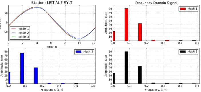
An example of spectrum of level oscillations on station LIST-auf-SYLT from model results presented in Fig. 5. The am- plitude of theM2 wave on quad meshes (MESH-1 and MESH-3) slightly exceeds 80 cm and is a bit smaller on MESH-2.
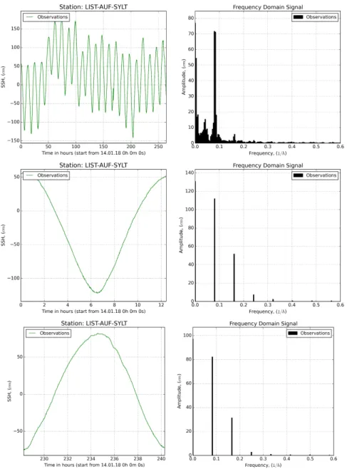
Similar behavior is seen for the second harmonics (M4) expressing nonlinear effects in this region. We tried to compare model simulation with the observations (https://www.pegelonline.wsv.de/gast/start/). For comparison, the observations were taken for 15
the first half of January, 2018. Figure 6 presents the range of fluctuations for the whole period. As is seen, the main tidal wave M2has a smaller amplitude (about 70 cm) than in simulations. However, the high-frequency part of the spectrum is very noisy because of atmospheric loading and winds. If the analysis is performed for separate tidal cycles in cases of strong wind and no-wind, the correspondence with observation is recovered in the second case.
Of particular interest is the convergence of solution on different meshes. For comparison the solutions simulated on MESH-2 20
and -3 were interpolated to the MESH-1. The comparison was performed for the full tidal cycle and is shown in Fig. 7 which presents the histograms of the differences.
For the solutions on MESH-1 and MESH-3 values at more than 80%of points agree within the range of±1 cm for the elevation (the maximum of tidal wave exceeds 1 m) and within the range of±1 cm/s for the velocity (the maximum horizontal velocity is about 120 cm/s). Thus the agreement between simulations on quadrilateral MESH-1 and MESH-3 is also maintained 25
on a local level. The agreement becomes worse when comparing solutions on triangular MESH-2 and quadrilateral MESH-1.
Here the share of points with larger deviations is noticeably larger.
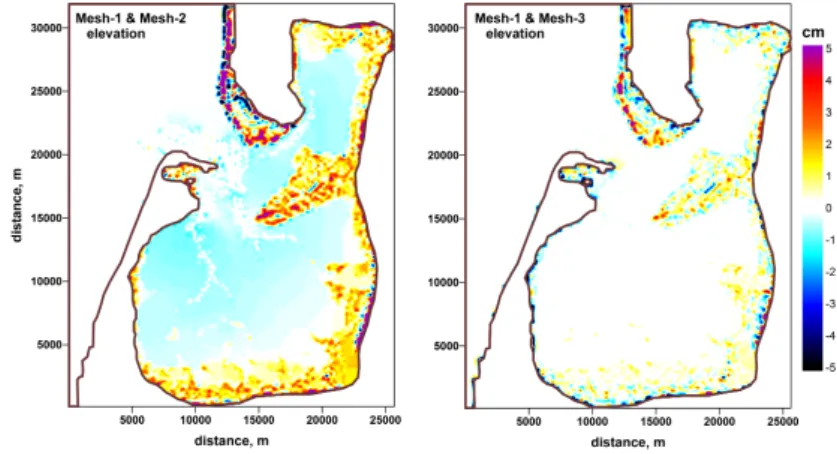
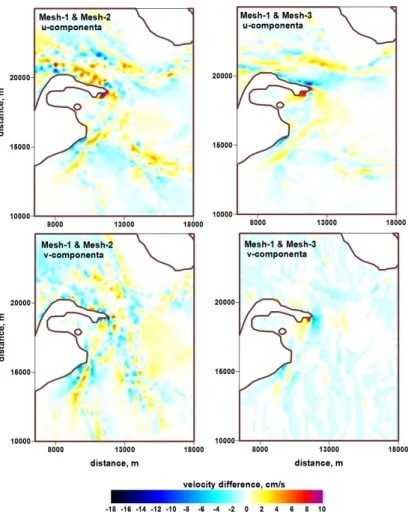
Spatial patterns of the differences for elevations and velocities simulated on different meshes are presented in Figs 8 and 9 respectively. Substantial differences for the elevation are located in wetting and drying zones. This is related to the sensitivity of the wetting and drying algorithm to the cell geometry. For the horizontal velocity the difference between the solutions is 30
defined by the resolution of bottom topography in the most energetically active zone on the quadrilateral meshes (see residual circulation in Fig. 4). The difference between the triangular grid and quadrilateral grid has a noisy character and is seen in the regions of strongest depth gradients.
5.2 South-East North Sea circulation
Here we present the results of realistic simulations of circulation in the southeastern part of the North Sea. The area of simula- tions is limited by the Dogger Bank and Horns Rev (Denmark) on the North and border between Belgium and the Netherlands on the west. It is characterized by complex bathymetry with strong tidal dynamics (Maßmann et al., 2010; Idier et al., 2017). The related estuarine circulation (Burchard et al., 2008; Flöser et al., 2011), strong lateral salinity and nutrient gradients and rivers 5
plumes (Voynova et al., 2017; Kerimoglu et al., 2017) are important aspects of this area. In our simulations, the mesh consists of mainly quadrilateral cells. The mesh is constructed with the Gmsh (Geuzaine and Remacle, 2009) using the Blossom-Quad method (Remacle et al., 2012). It includes 31406 quads and only 32 triangles. The mesh resolution (defined as the distance between vertices) varies between 0.5 - 1 km in the area close to the coast and Elbe estuary, coarsening to and 4 - 5 km at the open boundary. The mesh contains 5–σlayers in the vertical. The bathymetry from the EMODnet Bathymetry Consortium 10
(2016) has been used. Model runs were forced by 6 hourly atmospheric data from NCEP/NCAR Reanalysis (Kalnay et al., 1996) and dayly resolved observed river runoff (Radach and Pätsch , 2007; Pätsch and Lenhart, 2011). Salinity and temperature data on the open boundary were extracted from hindcast simulations based on TRIM-NP (Weisse et al., 2015). The sea surface elevation at the open boundary was prescribed in terms of amplitudes and phase forM2andM4tidal waves derived from the previous simulations of the North Sea (Maßmann et al., 2010; Danilov and Androsov, 2015). Data for temperature and salinity 15
from TRIM-NP model were used to initialize model runs for one year. The results of these runs were used as initial conditions for final simulation.
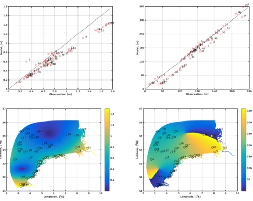
The validation of simulated amplitudes and phases ofM2 tidal wave is presented in Fig. 10. This wave is the main tidal constituent in this region. It enters the domain at the western boundary and propagates along the coast as a Kelvin wave. The phase field is characterized by two amphidromic points. We used the observed values from Andersen (2008) for the comparison.
20
The simulated amplitudes are generally slightly smaller than the observed ones (Fig. 10). The deviations in amplitudes can be explained by uncertainty in model bathymetry and the use of constant bottom friction coefficient. The phases ofM2wave are well reproduced by the model. We characterize its accuracy by the total vector error:
µ= 1 N
XN n=1
((A∗cosϕ∗−Acosϕ)2+ (A∗sinϕ∗−Asinϕ)2)1/2n ,
whereA∗,ϕ∗, andA,ϕ∗ are the observed and computed amplitudes and phases, respectively atN stations. The total vector 25
error is 0.24 m for 53 stations in the entire simulated domain which presents a reasonably good result for this region given the domain size. From the results of comparison it is seen that observations at some stations, such as station 7 in the open sea, differ considerably from the amplitude and phase at the close stations. The comparison will improve if such outlier stations are excluded.
To validate the simulated temperature and salinity we used data from the COSYNA data base (Baschek et al., 2016). The 30
model can represent both seasonal changes in sea surface temperature (SST) and salinity (SSS), as well as lateral gradients
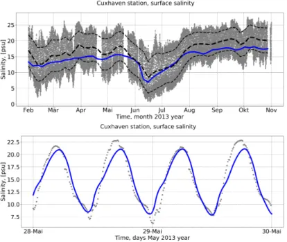
(not shown) reasonably well. The modeled and observed SSS for Cuxhaven station is presented in Fig. 11 for simulations with the Miura advection scheme.
The observations are from the station located in the mouth of the Elbe river near the coast. They are characterized by tidal amplitude in excess of 1.5 m, the horizontal salinity gradient of 0.35 PSU/km and an extended wetting and drying area around this station. Simulation is in good agreement with tidal filtered mean SSS (Fig. 11). The model represent well the summer flood 5
event during June - July months.
The (Fig. 12) shows the calculated surface salinity field in the part of the simulated domain at the time on June 26, 2013, in comparison with the observational data from (FerryBox (FunnyGirl) (Petersen, 2014). As can be seen from the plot, there is a high consistency of the simulated results with observational data.
6 Discussion 10
6.1 Triangles vs. quads: numerical performance
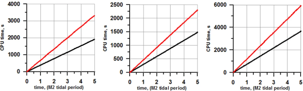
We examine the computational efficiency by comparing the CPU time needed to simulate 5 tidal periods ofM2–wave on MESH-1 and MESH-2 in the Sylt-Rømø experiment, as presented on Fig. 13. The number of vertices of the quadrilateral MESH-1 is approximately∼1.13of that of triangular MESH-2, but the numbers of elements relate as∼0.57. We have found that the total CPU times are in approximate ratio 1.62 (triangles/quads). The simulations were performed with the same time 15
steps.
The 3D velocity part takes approximately the same CPU time as the computation of vertically averaged velocity and eleva- tion (external mode). Operations on elements, which include the Coriolis and bottom friction terms as well as computations of gradients of velocity and scalars, are approximately twice cheaper on quadrilateral meshes, as expected. Computations of viscosity and momentum transport are carried out in a cycle over edges which is 1.5 times shorter for meshes made of quadri- 20
lateral elements, which warrants a similar gain of∼1.5in performance on quadrilateral meshes. In our simulation, the net gain was∼1.62times on MESH-1 compared to MESH-2, even despite the fact that number of vertices is 13% larger on MESH-2.
Model is stable on the quadrilateral meshes with smaller horizontal viscosity, which is also an advantage.
6.2 Triangles vs. quads: Open boundaries
The presence of open boundaries is a distinctive feature of regional models. The implementation of robust algorithms for the 25
open boundary is more complicated on unstructured triangular meshes than on structured quadrilateral meshes. For example, it is more difficult to cleanly assess the propagation of perturbations toward the boundary in this case. In addition, spurious inertial modes can be excited on triangular meshes in the case of cell-vertex discretization used by us, which in practice leads to additional instabilities in the vicinity of open boundary. The ability to use hybrid meshes is very helpful in this case. Indeed, even if the mesh is predominantly triangular, the vicinity of open boundary can be constructed of quadrilateral elements.
30
We illustrate the improvements of the dynamics in the vicinity of open boundary by simulating baroclinic tidal dynamic in an idealized channel with an underwater sill. The channel is 12 km in length and 3 km in width, with the maximum depth of 200 m near the open boundary. The sill with the height of 150 m in located in the central part of the channel. The flow is forced at the open boundaries by a tide with the period ofM2-wave and amplitude of 1 cm, applied in antiphase. The left part of the channel contains denser waters than the right one.
5
Three meshes were used for these simulations. The first one is a quadrilateral mesh with the horizontal resolution of 200 m refined to 20 m in the vicinity of the underwater sill. The second one is a purely triangular mesh obtained from the quadrilateral mesh by splitting quads into triangles. The third mesh is predominantly triangular, but for the zones close to the open boundary where it is quadrilateral too.
Fig. 14 illustrates that at time close to the maximum of the inflow (8h 20m), a strong computational instability due to the 10
interaction between baroclinic and barotropic flow components evolves on the right open boundary on the triangular mesh, leading eventually to the blow-up of the solution (see the left insert). However, replacing triangles in a small domain adjacent to the open boundary with quadrilateral cells we stabilize the numerical solution (see the right insert), for it allows us to cleanly handle the directions normal and tangent to the boundary.
7 Conclusions 15
We described the numerical implementation of three-dimensional unstructured-mesh model FESOM-C, relying on FESOM2 and intended for coastal simulations. The model is based on a finite-volume cell-vertex discretization and works on hybrid unstructured meshes composed of triangles and quads.
We illustrated the model performance with two test simulations.
Sylt-Rømø Bight is a closed Wadden Sea basin, characterized by a complex morphometry and high tidal activity. A sensitiv- 20
ity study was carried out to elucidate the dependence of simulated surface elevation and horizontal velocity on mesh type and quality. The elevation simulated in zones of wetting and drying may depend on the mesh structure, which may lead to distinc- tions in the simulated energy on different meshes. The total energy comparison shows that on the triangular MESH-2, having approximately the same number of vertices as MESH-1, the solution is more dissipative, for higher dissipation is generally needed to stabilize it against spurious inertial modes.
25
The second experiment deals with the southeastern part of the North Sea. Computation relied on the boundary information from hindcast simulations by the TRIM-NP, and realistic atmospheric forcing from NCEP/NCAR. Modeling results agree both qualitatively and quantitatively with observations for the full period of simulation.
Future development of the FESOM-C will include coupling with the global FESOM2 (Danilov et al., 2017), addition of monotonic high-order schemes and sea ice of FESOM2, and various modules that would increase functionality of FESOM-C.
30
Code and data availability. The version of FESOM-C used to carry out simulations reported here can be accessed from https://gitlab.dkrz.de/
a270101/FESOM-NF/ after registration. The simulation results can be obtained from the authors on request.
References
Andersen, O.B., Personal communication, 2008.
Androsov, A.A., Klevanny, K.A., Salusti, E.S., Voltzinger, N.E.: Open boundary conditions for horizontal 2-D curvilinear-grid long-wave dynamics of a strait, Advances in Water Resources, 18, 267–276, 10.1016/0309-1708(95)00017-D, 1995.
Barnier, B., Siefridt, L., Marchesiello, P.: Thermal forcing for a global ocean circulation model using a three-year climatology of ECMWF 5
analyses, J. Marine Syst., 6, 363–380, 10.1016/0924-7963(94)00034-9, 1995.
Baschek, B. et al.,: COSYNA – Coastal Observing System for Northern and Arctic Seas, Special Issue, Ocean Science and BioGeoScience, https://doi.org/10.5194/os2016-31, 2016.
Becherer, J., Burchard, H., Floeser, G., Mohrholz, V., Umlauf, L.: Evidence of tidal straining in well-mixed channel flow from micro-structure observations, Geophys. Res. Lett., 38, L17611, doi:10.1029/2011GL049005, 2011.
10
Benjamin, T. B.: Gravity currents and related phenomena, J. Fluid Mech., 31, 209–248, 1968.
Blumberg, A.F., and G.L. Mellor,: A Description of a three-dimensional coastal ocean circulation model. In: C.N.K. Mooers (Ed.), Three- dimensional Coastal Ocean Models, Coastal and Estuarine Sciences, 4, 1-16, 1987.
Burchard, H., Bolding, K., Ruiz-Villarreal, M.,: GOTM, a general ocean turbulence model. Theory, implementation and test cases. Tech.Rep.
EUR 18745 EN, European Commission, 1999.
15
Burchard, H., Bolding, K.,: GETM—a general estuarine transport model. Scientific documentation, Tech. Rep. EUR 20253 EN, European Commission, 2002.
Burchard, H., Floeser, G., Staneva, J., Badewien, T., Riethmueller, R.: Impact of Density Gradients on Net Sediment Transport into the Wadden Sea, Journal of Physical Oceanography, DOI: 10.1175/2007JPO3796.1, 2008.
Casulli V., Walters R.A.: An unstructured grid, three-dimensional model based on the shallow water equations. Int J Numer Meth Fluids 32:
20
331–348, 2000.
Cebeci, T. and Smith, A.M.O.: Analysis of Turbulent Boundary Layers. Academic Press, New York, 1974.
Chen, C., Liu, H., and Beardsley, R. C.: An unstructured, finite volume, three-dimensional, primitive equation ocean model: application to coastal ocean and estuaries, J. Atmos. Ocean. Tech., 20, 159–186, 2003.
Cheng, Y., Canuto V. M., and Howard A. M.: An improved model for the turbulent PBL, J. Atmos. Sci., 59, 1550–1565, 2002.
25
Danilov, S.: Two finite-volume unstructured mesh models for large-scale ocean modeling, Ocean Modell., 47, 14–25, doi:10.1016/j.ocemod.2012.01.004, 2012.
Danilov, S., Androsov, A.: Cell-vertex discretization of shallow water equations on mixed unstructured meshes, Ocean Dyn., 65, 33-47, doi:10.1007/s10236-014-0790-x, 2015.
Danilov, S., Sidorenko, D., Wang, Q., and Jung, T.: The Finite-volumE Sea ice–Ocean Model (FESOM2), Geosci. Model Dev., 10, 765-789, 30
https://doi.org/10.5194/gmd-10-765-2017, 2017.
Deleersnijder E., Roland M.: Preliminary tests of a hybrid numerical-asymptotic method for solving nonlinear advection-diffusion equations in a domain limited by a selfadjusting boundary, Mathematical and Computer Modelling, 17, 35-47, 1993.
Deleersnijder E.: Numerical mass conservation in a free-surface sigma coordinate marine model with mode splitting, Journal of Marine Systems, 4, 365-370, 1993.
35
Flöser, G., Burchard H., and Riethmüller, R.: Observational evidence for estuarine circulation in the German Wadden Sea, Cont. Shelf Res., 31, 1633–1639, 2011.
Fringer, O. B., Gerritsen, M., Street, R. L.: An unstructured-grid, finite-volume, nonhydrostatic, parallel coastal ocean simulator. Ocean Modelling 14, 139–173, 2006.
Gadd, A.J.: A split explicit integration scheme for numerical weather prediction, Q.J.R. Meteorol. Soc., 104(441), http://dx.doi.org/10.1002/qj.49710444103, 569–582, 1978.
Geuzaine C., and Remacle, J.-F.: Gmsh: a three-dimensional finite element mesh generator with built-in pre- and post-processing facilities, 5
International Journal for Numerical Methods in Engineering 79(11), 1309–1331, 2009.
Haidvogel, D. B. and Beckmann, A.: Numerical Ocean Circulation Modeling. Imperial College Press, 1999.
Higdon, R.L.: A comparison of two formulations of barotropic-baroclinic splitting for layered models of ocean circulation, Ocean Modelling, 24(1), 29–45, 2008.
Idier, D., Paris, F., Cozannet, G.L., Boulahya, F., Dumas, F.: Sea-level rise impacts on the tides of the European Shelf, Cont. Shelf Res., 137, 10
56–71, 2017.
Kalnay, E., et al.: The NCEP/NCAR 40-Year Reanalysis Project. Bulletin of the American Meteorological Society, 77, 437-471, 1996.
Kerimoglu, O., Hofmeister R., Maerz, J., Riethmüller, R., and Wirtz1, K.W.: The acclimative biogeochemical model of the southern North Sea, Biogeosciences, 14, 4499–4531, https://doi.org/10.5194/bg-14-4499-2017, 2017.
Lazure, P., Dumas F., An external–internal mode coupling for a 3D hydrodynamical model for applications at regional scale (MARS), 15
Advances in Water Resources, 31(2), 233-250, 2008.
Le Roux DY.: Spurious inertial oscillations in shallow-water models. J Comput Phys., 231, 7959-7987, 2012.
Lumborg, U. and Pejrup, M.: Modelling of cohesive sediment transport in a tidal lagoon an annual budget, Mar. Geol., 218, 1–16, 2005.
Luyten, P.J., Jones, J.E., Proctor, R., Tabor, A. and Wild-Allen, K.: COHERENS—A coupled hydrodynamical–ecological model for regional and shelf seas, user documentation. MUMM Rep. 911, 1999.
20
Marchesiello, P., McWilliams J.C., Shchepetkin, A.: Open boundary conditions for long-term integration of regional oceanic models, Ocean Modelling, 3(1), 1–20, 10.1016/S1463-5003(00)00013-5, 2001.
Maßmann, S., Androsov, A. and Danilov, S.: Intercomparison between finite element and finite volume approaches to model North Sea tides, Continental Shelf Research, 30 (6), 680–691, doi: 10.1016/j.csr.2009.07.004, 2010.
Miura, H.: An upwind-biased conservative advection scheme for spherical hexagonal-pentagonal grids, Mon. Wea. Rev., 135, 4038–4044, 25
2007.
Pätsch, J., Lenhart, H.J.: Daily Loads of Nutrients, Total Alkalinity, Dissolved Inorganic Carbon and Dissolved Organic Carbon of the European Continental Rivers for the Years 1977-2009. Institut für Meereskunde, Universität Hamburg, 2011.
Peterson W.,: Ferrybox systems: State-of-the-art in europe and future development. Journal of Marine Systems, 140:4 – 12, 2014. 5th Ferrybox Workshop - Celebrating 20 Years of Alg@line.
30
Phillips, N.A.: A coordinate system having some special advantages for numerical forecasting, J. Meteorol., 14, 184–185, 1957.
Purkiani, K., Becherer, J., Flöser, G., Gräwe, U., Mohrholz, V., Schuttelaars, H.M., Burchard, H.: Numerical analysis of stratification and destratification processes in a tidally energetic inlet with an ebb tidal delta, Journal of Geophysical Research: Oceans, 120, 10.1002/2014JC010325, 2014.
Radach, G., Pätsch, J.: Variability of continental riverine freshwater and nutrient inputs into the North Sea for the years 1977–2000 and its 35
consequences for the assessment of eutrophication Estuaries and Coasts, 30(1), 66-81, 2007.
Raymond, H.W., Kuo, L.H.: A radiation boundary condition for multi-dimensional flows, Quarterly Journal of the Royal Meteorological Society, 110, 535–551, 10.1002/qj.49711046414, 1984.
Reid R. O.: Modification of the quadratic bottom-stress law for turbulent channel flow in the presence of surface wind-stress. U.S. Army Corps of Engineers, Beach Erosion Board. Tech. Memo., 3, 33, 1957.
Remacle, J.-F., Lambrechts, J., Seny, B., Marchandise, E., Johnen A., Geuzainet, C.: Blossom-Quad: A non-uniform quadrilateral mesh generator using a minimum-cost perfect-matching algorithm, Intern. J. Numer. Meth. Eng., 89, 1102–1119, 2012.
Ruiz-Villarreal, M., Bolding, K., Burchard, H., Demirov, E.: Coupling of the GOTM turbulence module to some three-dimensional ocean 5
models. Marine Turbulence: Theories, Observations, and Models Results of the CARTUM Project, 225–237, 2005
Shchepetkin, A.F., McWilliams J.C., The Regional Ocean Modeling System: A split-explicit, free-surface, topography following coordinates ocean model, Ocean Modelling, 9, 347–404, 2005.
Stelling, G.S., Duinmeijer, S.P.A.: A staggered conservative scheme for every Froude number in rapidly varied shallow water flows, Int. J.
Numer. Meth. Fluids, 43(12), http://dx.doi.org/10.1002/fld.537, 1329–1354, 2003.
10
Zhang, Y., Baptista, A.M., 2008. SELFE: A semi-implicit Eulerian-Lagrangian finite-element model for cross-scale ocean circulation. Ocean Modelling 21, 71–96.
Umlauf, L., Burchard, H., 2005. Second-order turbulence closure models for geophysical boundary layers. A review of recent work. Conti- nental Shelf Research 25, 795–827.
Umlauf, L., Burchard, H., Bolding, K., 2005. General Ocean Turbulence Model. Scientific documentation. v3.2. Marine Science Reports 63, 15
274.
Umlauf, L., Burchard, H., Bolding, K., 2007. GOTM. Sourcecode and Test Case Documentation. Version 4.0.
Voltzinger N.E.: Long Waves on Shallow Water, Gidrometioizdat, Leningrad, 1985, 160. (in russian).
Voynova, Y. G., Brix, H., Petersen, W., Weigelt-Krenz, S., and Scharfe, M.: Extreme flood impact on estuarine and coastal biogeochemistry:
the 2013 Elbe flood, Biogeosciences, 14, 541–557, https://doi.org/10.5194/bg-14-541-2017, 2017.
20
Weisse R., Bisling P., Gaslikova L., Geyer B., Groll N., Hortamani M., Matthias V., Maneke M., Meinke I., Meyer E., Schwichten- berg F., Stempinski F., Wiese F., Wöckner-Kluwe K.: Climate services for marine applications in Europe. Earth Perspectives 2:3, doi:10.1186/s40322-015-0029-0, 2015.
Wang, Q., Danilov, S., Sidorenko, D., Timmermann, R., Wekerle, C., Wang, X., Jung, T., and Schröter, J.: The Finite Element Sea Ice-Ocean Model (FESOM) v.1.4: formulation of an ocean general circulation model, Geosci. Model Dev., 7, 663– 693, doi:10.5194/gmd-7-663- 25
2014, 2014.
Zhang, Y. J., Ye, F., Stanev, E. V., and Grashorn, S.: Seamless cross-scale modeling with SCHISM, Ocean Modelling, 102, 64–81, https://doi.org/10.1016/j.ocemod.2016.05.002, 2016
Figure 1.Schematic of mesh structure. Velocities are located at centroids (red circles) and elevation at vertices (blue circles). A scalar control volume associated with vertexv1is formed by connecting neighboring centroids to edge centers. The control volumes for velocity are the triangles/quads themselves. The lines passing through two neighboring centroids (e. g.,c1 andc2) are broken in a general case at edge centers. Their fragments are described by the left and right vectors directed to centroids (slandsrfor edgee). Edgeeis defined by its two verticesv1andv2and is considered to be directed to the second vertex. It is also characterized by two elementsc1andc2to the left and to the right respectively.