https://doi.org/10.5194/gmd-12-1009-2019
© Author(s) 2019. This work is distributed under the Creative Commons Attribution 4.0 License.
FESOM-C v.2: coastal dynamics on hybrid unstructured meshes
Alexey Androsov1,3, Vera Fofonova1, Ivan Kuznetsov1, Sergey Danilov1,4,5, Natalja Rakowsky1, Sven Harig1, Holger Brix2, and Karen Helen Wiltshire1
1Alfred Wegener Institute for Polar and Marine Research, Bremerhaven, Germany
2Institute of Coastal Research, Helmholtz-Zentrum Geesthacht, Geesthacht, Germany
3Shirshov Institute of Oceanology RAS, Moscow, Russia
4A. M. Obukhov Institute of Atmospheric Physics RAS, Moscow, Russia
5Jacobs University, Bremen, Germany
Correspondence:Alexey Androsov (alexey.androsov@awi.de) Received: 23 April 2018 – Discussion started: 25 July 2018
Revised: 8 December 2018 – Accepted: 15 February 2019 – Published: 21 March 2019
Abstract.We describe FESOM-C, the coastal branch of the Finite-volumE Sea ice – Ocean Model (FESOM2), which shares with FESOM2 many numerical aspects, in particu- lar its finite-volume cell-vertex discretization. Its dynamical core differs in the implementation of time stepping, the use of a terrain-following vertical coordinate, and the formulation for hybrid meshes composed of triangles and quads. The first two distinctions were critical for coding FESOM-C as an in- dependent branch. The hybrid mesh capability improves nu- merical efficiency, since quadrilateral cells have fewer edges than triangular cells. They do not suffer from spurious in- ertial modes of the triangular cell-vertex discretization and need less dissipation. The hybrid mesh capability allows one to use quasi-quadrilateral unstructured meshes, with triangu- lar cells included only to join quadrilateral patches of differ- ent resolution or instead of strongly deformed quadrilateral cells. The description of the model numerical part is comple- mented by test cases illustrating the model performance.
1 Introduction
Many practical problems in oceanography require regional focus on coastal dynamics. Although global ocean circula- tion models formulated on unstructured meshes may in prin- ciple provide local refinement, such models are as a rule based on assumptions that are not necessarily valid in coastal areas. The limitations on dynamics coming from the need to resolve thin layers, maintain stability for sea surface el- evations comparable to water layer thickness, or simulate
the processes of wetting and drying make the numerical ap- proaches traditionally used in coastal models different from those used in large-scale models. For this reason, combining coastal and large-scale functionality in a single unstructured- mesh model, although possible, would still imply a combina- tion of different algorithms and physical parameterizations.
Furthermore, on unstructured meshes, the numerical stabil- ity of open boundaries, needed in regional configurations, sometimes requires masking certain terms in motion equa- tions close to open boundaries. This would be an unneces- sary complication for a large-scale unstructured-mesh model that is as a rule global.
The main goal of the development described in this paper was to design a tool, dubbed FESOM-C, that is close to FE- SOM2 (Danilov et al., 2017) in its basic principles, but can be used as a coastal model. Its routines handling the mesh in- frastructure are derived from FESOM2. However, the time stepping, vertical discretization, and particular algorithms, detailed below, are different. FESOM-C relies on a terrain- following vertical coordinate (vs. the arbitrary Lagrangian–
Eulerian (ALE) vertical coordinate of FESOM2), but takes a step further with respect to the mesh structure. It is designed to work on hybrid meshes composed of triangles and quads.
Some decisions, such as the lack of the ALE at the present stage, are only motivated by the desire to keep the code as simple as possible through the initial phase of its develop- ment and maintenance. The code is based on the cell-vertex finite-volume discretization, the same as FESOM2 (Danilov et al., 2017) and FVCOM (Chen et al., 2003). It places scalar
quantities at mesh vertices and the horizontal velocities at cell centroids.
Our special focus is on using hybrid meshes. In essence, the capability of hybrid meshes is built on the finite-volume method. Indeed, computations of fluxes are commonly im- plemented as cycles over edges, and the edge-based infras- tructure is immune to the polygonal type of mesh cells. How- ever, because of staggering, it is still convenient to keep some computations on cells, which then depend on the cell type.
Furthermore, high-order transport algorithms might also be sensitive to the cell geometry. We limit the allowed polygons to triangles and quads. Although there is no principal limi- tation on the polygon type, triangles and quads are versatile enough in practice for the cell-vertex discretization. Our mo- tivation for using quads is twofold (Danilov and Androsov, 2015). First, quadrilateral meshes have 1.5 times fewer edges than triangular meshes, which speeds up computations be- cause cycles over edges become shorter. The second reason is the intrinsic problem of the triangular cell-vertex discretiza- tion – the presence of spurious inertial modes (see, e.g., Le Roux, 2012) and decoupling between the nearest horizontal velocities. Although both can be controlled by lateral vis- cosity, the control leads to higher viscous dissipation over the triangular portions of the mesh. The hybrid meshes can be designed so that triangular cells are included only to op- timally match the resolution or are even absent altogether.
For example, FESOM-C can be run on curvilinear meshes combining smooth changes in the shape of quadrilateral cells with smoothly approximated coastlines. One can also think of meshes for which triangular patches are only used to pro- vide transitions between quadrilateral parts of different reso- lution, implementing an effective nesting approach.
Many unstructured-mesh coastal ocean models were pro- posed recently (e.g., Casulli and Walters, 2000; Chen et al., 2003; Fringer et al., 2006; Zhang and Baptista, 2008; Zhang et al., 2016). It will take some time for FESOM-C to catch up in terms of functionality. The decision on the development of FESOM-C was largely motivated by the desire to fit in the existing modeling infrastructure (mesh design, analysis tools, input–output organization), and not by any deficiency in ex- isting models. The real workload was substantially reduced through the use or modification of the existing FESOM2 rou- tines.
We formulate the main equations and their discretization in the three following sections. Section 5 presents results of test simulations, followed by a discussion and conclusions.
2 Model formulation 2.1 The governing equations
We solve standard primitive equations in the Boussinesq, hydrostatic, and traditional approximations (see, e.g., Mar- shall et al., 1997). The solution is sought in the domain
Qb=Q× [0, tf], wheretfis the time interval. The boundary
∂Qof domainQis formed by the free water surface, the bot- tom boundaries, and lateral boundaries composed of the solid part∂Q1 and the open boundary∂Q2,Q= {x, y, z;x, y∈
,−h(x, y)≤z < ζ (x, y, t )}, 0≤t≤tf. Hereζ is the sur- face elevation andhthe bottom topography. We seek the vec- tor of unknownq=(u, w, ζ, T , S), whereu=(u, v)is the horizontal velocity,w the vertical velocity, T the potential temperature, andSthe salinity, satisfying the equations
∂u
∂t + ∂
∂xi
(uui)+ ∂
∂z(uw)+ 1 ρ0
∇p+fk×u
= ∂
∂zϑ∂u
∂z + ∇ ·(K∇)u, (1)
∇ ·u+ ∂
∂zw=0, (2)
∂p
∂z = −gρ, (3)
∂2j
∂t + ∂
∂xi
(ui2j)+ ∂
∂z(w2j)= ∂
∂zϑ2∂2j
∂z
+ ∇(K2∇)2j. (4)
Herei=1,2,x1=x,x2=y,u1=u, andu2=v, and sum- mation is implied over the repeating indicesi;pis the pres- sure; andj=1,2 with 21=T and22=S represents the potential temperature and salinity, respectively. The seawater density is determined by the equation of stateρ=ρ(T , S, p), andρ0is the reference density;f is the Coriolis parameter;k is the vertical unit vector;ϑandKare the coefficients of ver- tical and horizontal turbulent momentum exchange, respec- tively;ϑ2 andK2 are the respective diffusion coefficients;
andgis the acceleration due to gravity.
Writing
ρ(x, y, z, t )=ρ0+ρ0(x, y, z, t ), (5) whereρ0 is the density fluctuation, we obtain, integrating Eq. (3),
p−patm=
ζ
Z
z
ρgdz=gρ0(ζ−z)+g
ζ
Z
z
ρ0dz,
wherepatmis the atmospheric pressure. The horizontal pres- sure gradient is then expressed as the sum of barotropic, baro- clinic, and atmospheric pressure gradients:
ρ0−1∇p=g∇ζ+gρ0−1∇I+ρ0−1∇patm, I=
ζ
Z
z
ρ0dz. (6)
Note that horizontal derivatives here are taken at fixedz.
2.2 Turbulent closures
The default scheme to compute the vertical viscosity and dif- fusivity in the system of Eqs. (1)–(4) is based on the Prandtl–
Kolmogorov hypothesis of incomplete similarity. According to it, the turbulent kinetic energy b, the coefficient of tur- bulent mixing ϑ, and dissipation of turbulent energy ε are connected as ϑ=l
√
b, where l is the scale of turbulence, ϑ2=cρϑ,ε=cεb2/ϑ, andcε=0.046 (Cebeci and Smith, 1974). Prandtl’s numbercρ is commonly chosen as 0.1 and sets the relationship between the coefficients of turbulent dif- fusion and viscosity. The equation describing the balance of turbulent kinetic energy is obtained by parameterizing the en- ergy production and dissipation in the equation for turbulent kinetic energybas
∂b
∂t −ϑ
|uz|2+cρgρ0−1∂ρ
∂z
+cεb2/ϑ=αb
∂
∂zϑ∂b
∂z, (7) with the boundary conditions
b|h=B1|u|2, ϑ bz|ζ =γζu3∗ζ,
where αb=0.73, B1=16.6, and γζ =0.4×10⁻³; u∗ζ= (ρ/ρa)1/2u∗is the dynamical velocity in water near the sur- face,ρathe air density, andu∗the dynamic velocity of water on the interface between air and water.
Dissipative term is written as b2/ϑ=
2bν+1bν−(b2)ν /ϑν,
whereνis the index of iterations. Equation (7) is solved by a three-point Thomas scheme in the vertical direction with the boundary conditions given above. Iterations are carried out until convergence determined by the condition
max
bν+1−bν /bν
< $,
where$ is a small valueO(10−6). More details on the so- lution of this equation are given in Voltzinger et al. (1989).
To determine the turbulence scalelin the presence of sur- face and bottom boundary layers we use the Montgomery formula (Reid, 1957):
l= κ HZhZζ,
where H=h+ζ is the full water depth, Zh=z+h+zh, Zζ= −z+ζ+zζ,κ'0.4 is the von Kármán constant,zthe layer depth, andzhandzζ are the roughness parameters for the bottom and free surface, respectively. To remove turbu- lent mixing in layers that are distant from interfaces we mod- ify the Montgomery formula by introducing the cutoff func- tionZ0=1−β1H−2ZhZζ, 0≤β1≤4 (Voltzinger, 1985):
l= κ
HZhZζZ0.
In addition to the default scheme, one may select a scheme provided by the General Ocean Turbulence Model (GOTM) (Burchard et al., 1999) implemented into the FESOM-C code for computing vertical eddy viscosity and diffusion for mo- mentum and tracer equations. GOTM includes large number of well-tested turbulence models with at least one member of every relevant model family (empirical models, energy mod- els, two-equation models, algebraic stress models, K-profile parameterizations, etc.) and treats every single water column independently. An essential part of GOTM includes one- point second-order schemes (Umlauf and Burchard, 2005;
Umlauf et al., 2005, 2007).
2.3 Bottom friction parameterization
The model uses either a constant bottom friction coefficient Cd, or it is computed through the specified bottom roughness heightzh. The first option is preferable if the vertical reso- lution everywhere in the domain does not resolve the loga- rithmic layer or when the vertically averaged equations are solved. In the second option the bottom friction coefficient is computed according to Blumberg and Mellor (1987) and has the following form:
Cd=(ln((0.5hb+zh) /zh) /κ)−2,
wherehbis the thickness of the bottom layer. It is also pos- sible to prescribe Cd or zh as a function of the horizontal coordinate at the initialization step.
2.4 Boundary conditions
The boundary conditions for the dynamical Eqs. (1)–(2) are those of no-slip on the solid boundary∂Q1,
u
∂Q1 =0.
As is well known, the formulation of open boundary con- ditions faces difficulties. They are related to either the lack or incompleteness of information demanded by the theory, for example on velocity components at the open boundary.
Furthermore, whatever the external information, it may con- tradict the solution inside the computational domain, leading to instabilities that are frequently expressed as small-scale vortex structures forming near the open boundary. The pro- cedure reconciling the external information with the solution inside the domain becomes of paramount importance. We use two approaches. The first one is to use a function whereby ad- vection and horizontal diffusion are smoothly tapered to zero in the close vicinity of open boundary∂Q2. Such tapering makes the equations quasi-hyperbolic at the open boundary so that the formulation of one condition (for example, for the elevation,ζ
∂Q2 =ζ0) is possible (Androsov et al., 1995).
The other approach is to adapt the external information. It is applied to scalar fields and will be explained further.
Note that despite simplifications, barotropic and baroclinic perturbations may still disagree at the open boundary, leading
to instabilities in its vicinity. In this case an additional buffer zone is introduced with locally increased horizontal diffusion and bottom friction.
Dynamic boundary conditions on the top and bottom spec- ify the momentum fluxes entering the ocean. Neglecting the contributions from horizontal viscosities, we write
ϑ∂u
∂z
ζ =τζ/ρ0, ϑ∂u
∂z|−h =τh/ρ0=Cd|uh|uh.
The first one sets the surface momentum flux to the wind stress at the surface (τζ), and the second one sets the bottom momentum flux to the frictional flux at the bottom (τh), with uhthe bottom velocity.
Now we turn to the boundary conditions for the scalar quantities obeying Eq. (4). This is a three-dimensional parabolic equation and the boundary conditions are deter- mined by its leading (diffusive) terms. We impose the no-flux condition on the solid boundary∂Q1and the bottomz= −h.
The conditions at the open boundary ∂Q2 are given for outflow and inflow; see, e.g., Barnier et al. (1995) and March- esiello et al. (2001):
2t+a2x+b2y= −1
τ(2−20) ,
where 20 is the given field value, usually a climato- logical one or relying on data from a global numerical model or observations. If the phase velocity components anda= −2t2x/G,b= −2t2y/G, andG= [(∂2/∂x)2+ (∂2/∂y)2]−1(Raymond and Kuo, 1984),2propagates out of the domain, and one setsτ =τ0. If it propagates into the domain,a andb are set to zero and τ=τ0, with τ0τ0. The parameter τ is determined experimentally and com- monly is from hours to days. In the FESOM-C such an adap- tive boundary condition is routinely applied for temperature and salinity, yet it can also be used for any components of a solution.
At the surface the fluxes are due to the interaction with the atmosphere:
ϑ2
∂T
∂z
ζ = ˆQ(x, y, t )/ρ0cp, (8) ϑ2
∂S
∂z
ζ =0, (9) where Qˆ is the heat flux excluding shortwave radiation, which has been included as a volume heat source in the tem- perature equation, withcpthe specific heat of seawater. The impact of the precipitation–evaporation has been included as a volume source in the continuity equation. In the presence of rivers, their discharge is added either as a prescribed inflow at the open boundary in the river mouth or as volume sources of mass, heat, and momentum distributed in the vicinity of the open boundary. In the first case it might create an initial shock in elevation, so the second method is safer.
3 Temporal discretization
As is common in coastal models, we split the fast and slow motions into, respectively, barotropic and baroclinic subsys- tems (Lazure and Dumas, 2008; Higdon, 2008; Gadd, 1978;
Blumberg and Mellor, 1987; Deleersnijder and Roland, 1993). The reason for this splitting is that surface gravity waves (external mode) are fast and impose severe limitations on the time step, whereas the internal dynamics can be com- puted with a much larger time step. The time step for the external modeτ2-Dis limited by the speed of surface grav- ity waves, and that for the internal mode,τ3-D, by the speed of internal waves or advection. The ratioMt =τ3-D/τ2-Dde- pends on applications, but is commonly between 10 and 30.
In practice, additional limitations are due to vertical advec- tion or wetting and drying processes. We will further use the indiceskandnto enumerate the internal and external time steps, respectively.
The numerical algorithm passes through several stages. In the first stage, based on the current temperature and salin- ity fields (time step k), the pressure is computed from hy- drostatic equilibrium Eq. (6) and then used to compute the baroclinic pressure gradientρ0−1∇p=g∇ζk+gρ0−1∇Ik+ ρ0−1∇patm. We use an asynchronous time stepping, assum- ing that integration of temperature and salinity is half-step shifted with respect to momentum. The indexkonI implies that it is centered betweenkandk+1 of momentum integra- tion. The elevation in the expression above is taken at time stepk, which makes the entire estimate for ∇p only first- order accurate with respect to time.
At the second stage, the predictor values of the three- dimensional horizontal velocity are determined as
euk+1−uk=τ3-D(−fk×u− ∇ ·uu+ ∇ ·(K∇u))AB3
−τ3-Dρ0−1∇p+τ3-D∂zϑ ∂zeuk+1−τ3-D∂z(wu)AB3. HereK is the coefficient of horizontal viscosity, and AB3 implies the third-order Adams–Bashforth estimate. The hori- zontal viscosity operator can be made biharmonic or replaced with filtering as discussed in the next chapter.
To carry out mode splitting, we write the horizontal ve- locity as the sum of the vertically averaged oneu and the deviation thereof (pulsation)u0:
u=u+u0, u= 1
H
ζ
Z
−h
udz,
ζ
Z
−h
u0=0.
By integrating the system in Eqs. (1)–(3) vertically between the bottom and surface, with regard for the kinematic bound- ary conditions∂tζ+u∇ζ =won the surface,−u∇h=wat
the bottom, and time discretization, we get
ζn+1−ζn
+τ2-D∇(Hu)AB3=0,
un+1−un=τ2-D(−fk×u− ∇ ·u u+ ∇ ·(K∇u))AB3
−τ2-D(g∇ζ )AM4+τ2-D τζ/ρ0−τh
−τ2-DR03-D
−τ2-Dgρ0−1∇Ik.
Here a specific version of AB3 is used: uAB3=(3/2+ β)uk−(1/2+2β)uk−1+βuk−2, with β=0.281105 for stability reasons (Shchepetkin and McWilliams, 2005);
AM4 implies the Adams–Multon estimateζAM4=δζn+1+ (1−δ−γ−) ζn+γ ζn−1+ζn−2, taken with δ=0.614, γ =0.088, and =0.013 (Shchepetkin and McWilliams, 2005). In the equations aboveτζandτhare the surface (wind) and bottom stresses, respectively, and∇Iis the vertically in- tegrated gradient of baroclinic pressure. The termR03-Dcon- tains momentum advection and horizontal dissipation of the pulsation velocity integrated vertically:
R3-D0 = 1 Hk
ζ
Z
−h
∇ ·u0u0−
ζ
Z
−h
∇ · K∇u0
k
.
In this expressionHk is the total fluid depth at time stepk, Hk=h+ζk. This term is computed only on the baroclinic time step and kept constant through the integration of the internal mode.
The bottom friction is taken as τh=Cd|u|n
un+1−un
/Hn+1+Cd|euh|k+1euk+1h /Hn+1. The first part of bottom friction is needed to increase stabil- ity, while the second part estimates the correct friction, with euk+1h the horizontal velocity vector in the bottom cell on the predictor time step.
The system of vertically averaged equations is stepped ex- plicitly (except for the bottom friction) throughMttime steps of durationτ2-D(indexn) to “catch up” thek+1 baroclinic time step. The update of elevation is made first, followed by the update of vertically integrated momentum equations.
At the “corrector” step, the 3-D velocities are corrected to the surface elevation atk+1:
uk+1= 4k
i
4k+1
i
euk+1+
uk+1−uP ,
with uP= 1
Hk+1
Pζ
−h euk+14k
i
, where i is the vertical in- dex. Here4k
i and4k+1
i are the thicknesses of theith layer calculated on respective baroclinic time steps. The layer thickness is4k
i = 4iHk, where4i is the unperturbed verti- cal grid spacing. This correction removes the barotropic com- ponent of the predicted velocity and combines the result with the computed barotropic velocity. We will suppress the layer indexiwhere it is unambiguous.
The final step in the dynamical part calculates the trans- formed vertical velocitywk+1from 3-D continuity Eq. (2).
It is used in the next predictor step. Note that in the predictor step the computations of vertical viscosity are implicit.
New horizontal velocities, the so-called “filtered” ones, are used for advection of a tracer. They are given by the sum of the filtered depth mean and the baroclinic part of the “pre- dicted” velocities (Deleersnijder, 1993),
uk+1F = 4k
i
4k+1
i
euk+1+
uF−uP ,
with uF = 1
MtHk+1
Pn=Mt
n=1 unHn
. The procedure of “fil- tering” removes possible high-frequency components in the barotropic velocity. It also improves accuracy because it in essence works toward centering the contribution of the ele- vation gradient. Once the filtered velocity is computed, the vertical velocity is updated to match it.
The equation for temperature is taken in the conservation form
4k+1Tk+1
= 4kTk−τ3-D
h
∇ ·
uk+1F 4kT∗
+wFtTt∗−wFbTb∗i +D+τ3-DR+τ3-DC,
whereDcombines the terms related to diffusion,wFt, wFb, Tt, andTbare the vertical transport velocity and temperature on top and bottom of the layer, andT∗is computed through the second-order Adams–Bashforth estimate.Ris the bound- ary thermal flux (either from the surface or due to river dis- charge). The last term in the equation above is
C=T∂4i
∂t = −T
∇(4iuF)k+1+∂z(4iwF)k+1 .
Its two constituents combine to zero because of continuity.
Keeping this term makes sense if computations of advection are split into horizontal and vertical substeps. The salinity is treated similarly.
In simulations of coastal dynamics it is often necessary to simulate flooding and drying events. Explicit time stepping methods of solving the external mode are well suited for this (Luyten et al., 1999; Blumberg and Mellor, 1987; Shchep- etkin and McWilliams, 2005). The algorithm to account for wetting and drying will be presented in the next section. We only note that computations are performed on each time step of the external mode.
4 Spatial discretization
In the finite-volume method, the governing equations are in- tegrated over control volumes, and the divergence terms, by virtue of the Gauss theorem, are expressed as the sums of respective fluxes through the boundaries of control volumes.
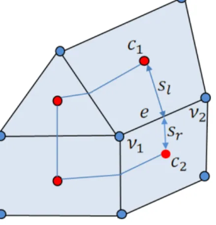
Figure 1.Schematic of mesh structure. Velocities are located at cen- troids (red circles) and elevation at vertices (blue circles). A scalar control volume associated with vertexv1is formed by connecting neighboring centroids to edge centers. The control volumes for ve- locity are the triangles and quads themselves. The lines passing through two neighboring centroids (e.g.,c1andc2) are broken in a general case at edge centers. Their fragments are described by the left and right vectors directed to centroids (sl andsr for edgee).
Edgeeis defined by its two verticesv1andv2and is considered to be directed to the second vertex. It is also characterized by two elementsc1andc2to the left and to the right, respectively.
For the cell-vertex discretization the scalar control volumes are formed by connecting cell centroids with the centers of edges, which gives the so-called median-dual control vol- umes around mesh vertices. The vector control volumes are the mesh cells (triangles or quads) themselves, as schemati- cally shown in Fig. 1.
The basic structure to describe the mesh is the array of edges given by their verticesv1andv2, and the array of two pointers c1 andc2 to the cells on the left and on the right of the edge. There is no difference between triangles, quads, or hybrid meshes in the cycles that assemble fluxes. Quads and triangles are described through four indices to the ver- tices forming them; in the case of triangles the fourth index equals the first one. The treatment of triangles and quads dif- fers slightly in computations of gradients as detailed below.
We will use symbolic notatione(c)for the list of edges form- ing cellc,e(v)for the list of edges connected to vertexv, and v(c)for the list of vertices defining cell of elementc.
In the vertical direction we introduce a σ coordinate (Phillips, 1957):
σ =z+h
h+ζ, 1≤σ≤0.
The lower and upper horizontal faces correspond to the planesσ =0 andσ=1, respectively. The vertical grid spac- ing is defined by the selected set of σi. The spacing ofσi is horizontally uniform in the present implementation (but it can be varying) and can be selected as equidistant or based on a parabolic function with high vertical resolution near the
surface and bottom in the vertical, σi= −
i−1 N−1
%
+1,
whereNis the number of vertical layers. Here%=1(2)gives the uniform (parabolic) distribution of vertical layers. One more possibility to use refined resolution near the bottom or surface is implemented through the formula by Burchard and Bolding (2002):
σi= tanhh
Lh+Lζ(N−i) (N−1)−Lh
i
+tanhLh
tanhLh+tanhLζ −1,
whereLh andLζ are the number of layers near the bottom and surface, respectively.
The vertical grid spacing is recalculated on each baroclinic time step for the vertices whereζ is defined. It is interpolated from vertices to cells and to edges. The vectors of horizontal velocity and tracers are located in the middle of vertical lay- ers (indexi+1/2), but the vertical velocity is at full layers.
4.1 Divergence and gradients
Thedivergence operatoron scalar control volumes is com- puted as
Z
v
∇ ·(4u)dS= X
e=e(v)
(4un`)l+(4un`)r ,
where the cycle is over edges containing vertexv, the indices l and r imply that the estimates are made on the left and right segments of the control volume boundary attached to the cen- ter of edgee,nis the outer normal, and`the length of the segment (see Fig. 1). With vectorssl andsrconnecting the midpoint of edgeewith the cell centers on the left and on the right, we get(n`)l=k×sl and similar, but with the minus sign for the right element (k is a unit vertical vector). The mean cell values, for example layer thickness on the cell, can be defined as4c=P
v=v(c)4vwcv, wherewcv=1/3 on tri- angles andwcv=Scv/Scfor quads (Sccell area andScv, the part of it in the scalar control volume around the vertex).
Gradients of scalarquantities are needed on cells and are computed as
Z
c
∇ζdS= X
e=e(c)
(n`ζ )e,
where summation is over the edges of cellc, the normal and length are related to the edges, andζis estimated as the mean over edge vertices.
Thegradients of velocitieson cells can be needed for the computation of viscosity and the momentum advection term.
They are computed through the least squares fit based on the velocities on neighboring cells:
L= X
n=n(c)
uc−un− αx, αy rcn2
=min.
Here rcn=(xcn, ycn) is the vector connecting the cen- ter of c to that of its neighbor n. Their solution can be reformulated in terms of two matrices (computed once and stored) with coefficientsacnx = xcnY2−ycnXY
/d and acny = ycnX2−xcnXY
/d, acting on velocity differences and returning the derivatives. Hered=X2Y2−(XY )2,X2= P
n=n(c)xcn2,Y2=P
n=n(c)ycn2, andXY =P
n=n(c)xcnycn. 4.2 Momentum advection
We implemented two options for horizontal momentum ad- vection in the flux form. The first one is linear reconstruction upwind based on cell control volumes (see Fig. 1). The sec- ond one is central and is based on scalar control volumes, with subsequent averaging to cells. In the upwind implemen- tation we write
Z
c
∇ ·(u4u)dS= X
e=e(c)
(un`4u)e.
For edgee, linear velocity reconstructions on the elements on its two sides are estimated at the edge center. One of the cells isc, and letnbe its neighbor acrosse. The respective velocity estimates will be denoted asuce andune, and up- wind will be written in the form 2u=uce(1+sgn(un))+ une(1−sgn(un)), whereun=n((uce+une)) /2.
The other form is adapted from Danilov (2012). It provides additional smoothing for momentum advection by comput- ing flux divergence for larger control volumes. In this case we first estimate the momentum flux term on scalar control volumes:
Z
v
∇ ·(u4u)dS= X
e=e(v)
(un`4u)l+(un`4u)r .
The notation here follows that for the divergence. No ve- locity reconstruction is involved. These estimates are then averaged to the centers of cells. In both variants of advection form the fluid thickness is estimated at cell centers.
4.3 Tracer advection
Horizontal advection and diffusion terms are discretized ex- plicitly in time. Three advection schemes have been imple- mented. The first two are based on linear reconstruction for control volume and are therefore second order. The linear re- construction upwind scheme and the Miura scheme (Miura, 2007) differ in the implementation of time stepping. The first needs the Adams–Bashforth method to be second order with respect to time. The scheme by Miura reaches this by esti- mating the tracer at a point displaced by uτ3-D/2. In both cases a linear reconstruction of the tracer field for each scalar control volume is performed:
2R(x, y)=20(xv, yv)+2x(x−xv)+2y(y−yv),
where20is the tracer value at vertex,2x and2y are the gradients averaged to vertex locations, andxvandyvthe co- ordinates of vertexv. The fluxes for scalar control volume faces associated with edgeeare computed as
X
e=e(v)
(un`42R)l+(un`42R)r .
The estimate of the tracer is made at the midpoints of the left and right segments and at points displaced byuτ3-D/2 from them, respectively.
The third approach used in the model is based on the gra- dient reconstruction. The idea of this approach is to estimate the tracer at mid-edge locations with a linear reconstruction using the combination of centered and upwind gradients:
2±e =2vi±`e(∇2)±e/2, where i=1,2 are the indices of edge vertices, and gradients are computed as
(∇2)+e =2
3(∇2)c+1
3(∇2)u and (∇2)−e =2
3(∇2)c+1 3(∇2)d.
Here, the upper index c means centered estimates, and u and d imply the estimates on the up- and down-edge cells.
The advective flux of scalar quantity2through the face of the scalar volume Qe=
(un`4)l+(un`4)r
associated with edgee, which leaves the control volumeν1(see Fig. 1), is
Qe2e=1
2Qe 2+e +2−e +1
2(1−γ )|Qe| 2+e +2−e , whereγ is the parameter controlling the upwind dissipation.
Takingγ=0 gives the third-order upwind method, whereas γ=1 gives the centered fourth-order estimate.
A quadratic upwind reconstruction is used in the vertical with the flux boundary conditions on surface (Eqs. 8 and 9) and zero flux at the bottom. Other options for horizontal and vertical advection, including limiters, will be introduced in the future.
The advection schemes are coded so that their order can be reduced toward the first-order upwind for a very thin wa- ter layer to increase stability in the presence of wetting and drying.
4.4 Viscosity and filtering
Consider the operator∇A∇u. Its computation follows the rule
Z
c
∇A∇udS= X
e=e(c)
A`(n∇u)e.
The estimate of velocity gradient on edgeeis symmetrized following the standard practice (Danilov, 2012) over the val- ues on neighboring cells. “Symmetrized” means that the es- timate on edgeeis the mean of horizontal velocity gradients
Figure 2. (a)The bathymetry of the Sylt–Rømø Bight (provided by Hans Burchard, personal communication, 2015) with the location of station List-auf-Sylt;(b)the regular quasi-quadrilateral MESH-1 (200 m; 16 089 vertices, 15 578 quads, and 176 triangles);(c)the triangular MESH-2 (14 193 vertices and 27 548 triangles); and(d)the irregular quadrilateral MESH-3 (35 639 vertices, 34 820 quads, and 31 triangles).
computed on elements candn (notation from article) with the common edgee:(∇u)e=((∇u)c+(∇u)n)/2. The con- sequence of this symmetrization is that on regular meshes (formed of equilateral triangles or rectangular quads) the in- formation from the nearest neighbors is lost. Any irregular- ity in velocity on the nearest cells will not be penalized. Al- though unfavorable for both quads and triangles, it has far- reaching implications for the latter: it cannot efficiently re- move the decoupling between the nearest velocities, which may occur for triangular cells. This fact is well known, and the modification of the scheme above that improves coupling between the nearest neighbors consists of using the identity n=rcn/|rcn| +(n−rcn/|rcn|) ,
wherercnis the vector connecting the centroid of cellscand n. The derivative in the direction ofrcnis just the difference
between the neighboring velocities divided by the distance, which is explicitly used to correctn∇u. It is easy to show that on rectangular quads or equilateral triangles (nandrcn are collinear) the second term of the expression above will disappear. This is the harmonic discretization and a bihar- monic version is obtained by applying the procedure twice.
A simpler algorithm is implemented to control grid-scale noise in the horizontal velocity. It consists of adding to the right hand for the momentum equation (2-D and 3-D flow) a term coupling the nearest velocities,
Fc= − 1
τf
X
n(c)
(un−uc) ,
whereτfis a timescale selected experimentally. On regular meshes this term is equivalent to the Laplacian operator. On
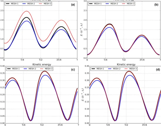
Figure 3.Potential and kinetic energy. Panels(a, c)are for the total area; panels(b, d)are for the area where the full depth exceeds 1 m.
general meshes it deviates from the Laplacian, yet after some trivial adjustments it warrants momentum conservation and energy dissipation (Danilov and Androsov, 2015).
4.5 Wetting and drying algorithm
For modeling wetting and drying we use the method pro- posed by Stelling and Duinmeijer (2003). The idea of this method is to accurately track the moving shoreline by em- ploying the upwind water depth in the flux computations. The criterion for a vertex to be wet or dry is taken as
wet, if Dwd=h+ζ+hl> Dmin dry, if Dwd=h+ζ+hl≤Dmin,
where Dmin is the critical depth and hl is the topography.
Each cell is treated as
wet, if Dwd=minhv(c)+maxζv(c)> Dmin
dry, if Dwd=minhv(c)+maxζv(c)≤Dmin,
wherehvandζvare the depth and sea surface height at the verticesv(c)of the cellc. When a cell is treated as dry, the velocity at its center is set to zero and no volume flux passes through the boundaries of scalar control volumes inside this cell.
5 Numerical simulations
In this section we present the results of two model experi- ments. The first considers tidal circulation in the Sylt–Rømø Bight. This area has a complex morphometry with big zones of wetting–drying and large incoming tidal waves. In this case our intention is to test the functioning of meshes of var- ious kinds. The second experiment simulates the southeast part of the North Sea. For this area, an annual simulation of barotropic–baroclinic dynamics with realistic boundary con- ditions on open and surface boundaries is carried out and compared to observations. We note that a large number of simpler experiments, including those in which analytical so- lutions are known, were carried out in the course of model development to test and tune the model accuracy and stabil- ity. Lessons learned from these were taken into account. We omit their discussion in favor of realistic simulations.
5.1 Sylt–Rømø experiment
To test the code sensitivity to the type of grid and grid qual- ity, we computed barotropic tidally driven circulation in the Sylt–Rømø Bight in the Wadden Sea.
It is a popular area for experiments and test cases (e.g., Lumborg and Pejrup, 2005; Ruiz-Villarreal et al., 2005; Bur- chard et al., 2008; Purkiani et al., 2014). The Sylt and Rømø islands are connected to the mainland by artificial dams, cre- ating a relatively small semi-enclosed bight with a circulation
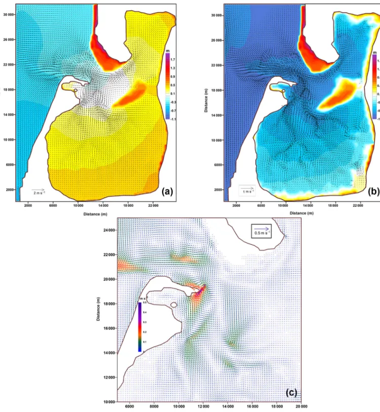
Figure 4. (a)Full ebb;(b)low water;(c)the residual circulation. Simulation was performed on MESH-1.
pattern well known from observations and modeling (e.g., Becherer et al., 2011; Purkiani et al., 2014). It is a tidally energetic region with a water depth down to 30 m, character- ized by wide intertidal flats and a rugged coastline. Water is exchanged with the open sea through a relatively narrow (up to 1.5 km wide) and deep (up to 30 m) tidal inlet, Lister Dyb.
The bathymetry data for the area were provided by Hans Bur- chard (personal communication, 2015) and are presented in Fig. 2.
We constructed three different meshes (Fig. 2) for our experiments. The first one is a nearly regular quadrilateral mesh, complemented by triangles that straighten the coast-
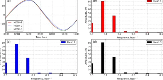
Figure 5. (a)Sea surface height (SSH) for one tidal period in the station List-auf-Sylt (see Fig. 2);(b)spectrum of the computedM2tidal sea level at station List-auf-Sylt on MESH-1;(c)spectrum on MESH-2; and(d)spectrum on MESH-3.
line (MESH-1). Its spatial resolution is 200 m. The second mesh is purely triangular (MESH-2) with resolution vary- ing from ∼820 to ∼90 m. The third mesh was generated by the Gmsh mesh generator (Geuzaine and Remacle, 2009) and includes 34 820 quads and 31 triangles with a minimum cell size of 30 m and maximum size of∼260 m (MESH-3).
All meshes have 21 nonuniform sigma layers in the vertical direction (refined near the surface and bottom). The wetting–
drying option is turned on. We apply thek−turbulence clo- sure model with transport equations for the turbulent kinetic energy and the turbulence dissipation rate using the GOTM library. The second-moment closure is represented by alge- braic relations suggested by Cheng et al. (2002). The exper- iment is forced by prescribing elevation due to anM2tidal wave at the open boundary (western and northern boundaries of the domain) provided by Hans Burchard (personal com- munication, 2015).
Simulations on each mesh were continued until reach- ing the steady state in the tidal cycle of the M2 wave. The last tidal period was analyzed. Quasi-stationary behavior is already established in the second tidal period. The simu- latedM2wave is essentially nonlinear during the tidal cycle judged by the difference in amplitude of two tidal half-cycles.
Figure 3 shows the behavior of potential and kinetic en- ergies in the entire domain, and the right panels show the energies computed over the areas deeper than 1 m. The re- sults are sensitive to the meshes, which is explained fur- ther. The smallest tidal energy is simulated on the triangular mesh (MESH-2). The reason is that with the same value of the timescaleτfin the filter used by us in these simulations, the effective viscous dissipation is much higher on a triangu- lar mesh than on quadrilateral meshes of similar resolution.
However, the solutions on quadrilateral meshes are also dif- ferent, and this time the reason is the difference in the details
of representing very shallow areas on meshes of various res- olution (MESH-3 is finer than MESH-1). The difference be- tween the simulations on two quadrilateral meshes is related to the potential energy and comes from the difference in the elevation simulated in the areas subject to wetting and drying (see Fig. 8). Note that the velocities and layer thickness are small in these areas, so the difference between kinetic ener- gies in Fig. 3c and d is small.
The average currents, sea level, and residual circulation simulated on MESH-1 are presented in Fig. 4. The results of this experiment show good agreement with the previously published results of Ruiz-Villarreal et al. (2005).
An example spectrum of level oscillations on station List- auf-Sylt from model results is presented in Fig. 5. The ampli- tude of theM2wave on quad meshes (MESH-1 and MESH- 3) slightly exceeds 80 cm and is a bit smaller on MESH-2.
Similar behavior is seen for the second harmonics (M4) ex- pressing nonlinear effects in this region. We tried to com- pare model simulation with the observations (https://www.
pegelonline.wsv.de/gast/start, last access: 28 February 2019).
For comparison, the observations were taken for the first half of January 2018. Figure 6 presents the range of fluctuations for the whole period. As is seen, the main tidal waveM2has a smaller amplitude (about 70 cm) than in simulations. How- ever, the high-frequency part of the spectrum is very noisy because of atmospheric loading and winds. If the analysis is performed for separate tidal cycles in cases of strong wind and no wind, the correspondence with observations is recov- ered in the second case.
Of particular interest is the convergence of the solution on different meshes. For comparison the solutions simulated on MESH-2 and MESH-3 were interpolated to MESH-1. The comparison was performed for the full tidal cycle and is
Figure 6. (a)Spectrum of the observation tidal sea level at station List-auf-Sylt (see Fig. 2) from 1 to 15 January 2018;(b)spectrum of the observation SSH for one tidal period with strong wind (1 January 2018); and(c)spectrum of the observation SSH for one tidal period with no wind (14 January 2018).
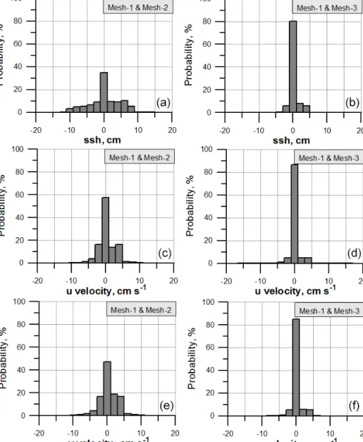
shown in Fig. 7, which presents histograms of the differ- ences.
For the solutions on MESH-1 and MESH-3 values at more than 80 % of points agree within the range of±1 cm for the elevation (the maximum tidal wave exceeds 1 m) and within the range of±1 cm s−1 for the velocity (the maximum hor- izontal velocity is about 120 cm s−1). Thus, the agreement between simulations on quadrilateral MESH-1 and MESH-3 is also maintained on a local level. The agreement becomes worse when comparing solutions on triangular MESH-2 and
quadrilateral MESH-1. Here the share of points with larger deviations is noticeably larger.
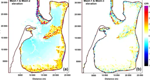
Spatial patterns of the differences for elevations and veloc- ities simulated on different meshes are presented in Figs. 8 and 9, respectively. Substantial differences for the elevation are located in wetting and drying zones. This is related to the sensitivity of the wetting and drying algorithm to the cell geometry. For the horizontal velocity the difference between the solutions is defined by the resolution of bottom topogra- phy in the most energetically active zone on the quadrilateral
Figure 7.Histograms of the difference between solutions for the tidal cycle of theM2wave on MESH-1 and MESH-2(a, c, e)and on MESH-1 and MESH-3(b, d, f). Top, middle, and bottom rows correspond to the difference in elevation and theuandvcomponents of velocity, respectively.
meshes (see residual circulation in Fig. 4). The difference between the triangular grid and quadrilateral grid has a noisy character and is seen in the regions of strongest depth gradi- ents.
5.2 Southeast North Sea circulation
Here we present the results of realistic simulations of cir- culation in the southeastern part of the North Sea. The area of simulations is limited by the Dogger Bank and Horns Rev (Denmark) on the north and the border between Bel- gium and the Netherlands on the west. It is characterized by complex bathymetry with strong tidal dynamics (Maß- mann et al., 2010; Idier et al., 2017). The related estuar- ine circulation (Burchard et al., 2008; Flöser et al., 2011),
strong lateral salinity, and nutrient gradients and river plumes (Voynova et al., 2017; Kerimoglu et al., 2017) are important aspects of this area. In our simulations, the mesh consists of mainly quadrilateral cells. The mesh is constructed with Gmsh (Geuzaine and Remacle, 2009) using the Blossom- Quad method (Remacle et al., 2012). It includes 31 406 quads and only 32 triangles. The mesh resolution (defined as the distance between vertices) varies between 0.5 and 1 km in the area close to the coast and Elbe estuary, coarsening to and 4–
5 km at the open boundary (Fig. 10). The mesh contains five sigma layers in the vertical.
Bathymetry from the EMODnet Bathymetry Consortium (2016) has been used. Model runs were forced by 6-hourly atmospheric data from NCEP/NCAR Reanalysis (Kalnay et
Figure 8.Spatial distribution of the elevation differences for a full tidal period for MESH-1 and MESH-2(a)and for MESH-1 and MESH- 3(b).
Figure 9.Spatial distribution of the difference between the hori- zontal velocities for the full tidal period of anM2wave:ucompo- nent(a, b);vcomponent(c, d). The differences are between MESH- 1 and MESH-2(a, c)and MESH-1 and MESH-3(b, d).
Figure 10.The area of the southeast North Sea experiment with mesh (black lines). The red dot indicates the position of the Cux- haven station. This mesh includes 31 406 quads and 32 triangles.
al., 1996) and daily resolved observed river runoff (Radach and Pätsch, 2007; Pätsch and Lenhart, 2011). Salinity and temperature data on the open boundary were extracted from hindcast simulations based on TRIM-NP (Weisse et al., 2015). The sea surface elevation at the open boundary was prescribed in terms of amplitudes and phase for M2 and M4tidal waves derived from the previous simulations of the North Sea (Maßmann et al., 2010; Danilov and Androsov, 2015). Data for temperature and salinity from the TRIM-NP model were used to initialize model runs for 1 year. The re- sults of these runs were used as initial conditions for a 10- month final simulation.
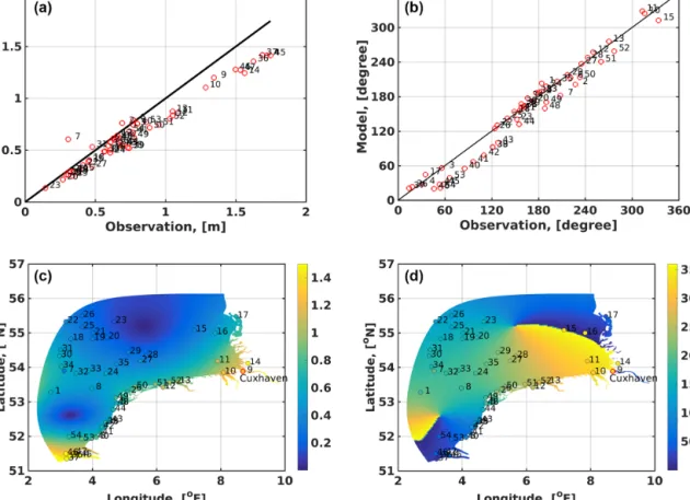
The validation of simulated amplitudes and phases of the M2tidal wave is presented in Fig. 11. This wave is the main tidal constituent in this region. It enters the domain at the western boundary and propagates along the coast as a Kelvin
Figure 11.The simulatedM2tidal map in the south North Sea experiment compared to observations. The amplitude is in meters(a, c)and phase(b, d)in degrees.(a, b)Model-to-observation graphs; the numbers correspond to station numbers shown in(c, d). The color shows the amplitude in(a)and phase in(b), and the filled circles show the observational data. The red circle indicates the position of Cuxhaven station.
The total vector error is 0.24 m for 53 stations.
wave. The phase field is characterized by two amphidromic points. We used the observed values from Ole Baltazar An- dersen (personal communication, 2008). for the comparison.
The simulated amplitudes are generally slightly smaller than the observed ones (Fig. 11). The deviations in amplitudes can be explained by uncertainty in model bathymetry and the use of a constant bottom friction coefficient. The phases of the M2wave are well reproduced by the model. We characterize its accuracy by the total vector error:
µ= 1 N
N
X
n=1
(A∗cosϕ∗−Acosϕ)2+(A∗sinϕ∗−Asinϕ)21/2 n ,
whereA∗,ϕ∗andA,ϕare the observed and computed ampli- tudes and phases, respectively, atNstations. The total vector error is 0.24 m for 53 stations in the entire simulated domain, which presents a reasonably good result for this region given the domain size. From the results of comparison it is seen that observations at some stations, such as station 7 in the open sea, differ considerably from the amplitude and phase at the close stations. The comparison will improve if such outlier stations are excluded.
To validate the simulated temperature and salinity we used data from the COSYNA database (Baschek et al., 2017) and ICES database (http://www.ices.dk, last access: 28 Febru- ary 2019). Comparisons of modeled surface temperature and salinity show good Pearson correlation coefficients of 0.98 and 0.9 with RMSD values of 1.24 and 0.98, respectively.
The model can represent both seasonal changes in sea sur- face temperature (SST) and salinity (SSS), as well as lateral gradients (not shown) reasonably well. The modeled and ob- served SSS for Cuxhaven station is presented in Fig. 12 for simulations with the Miura advection scheme.
The observations are from the station located in the mouth of the Elbe River near the coast. They are characterized by a tidal amplitude in excess of 1.5 m, a horizontal salin- ity gradient of 0.35 PSU km−1 (during spring tide up to 0.45 PSU km−1) (https://www.portal-tideelbe.de, last access:
28 February 2019, and Kappenberg et al., 2018), and an ex- tended wetting and drying area around this station. The sim- ulation is in good agreement with tidal filtered mean SSS (Fig. 12). The model represents the summer flood event dur- ing June–July well.
Figure 12.Modeled (blue line) and observed (gray dots and dashed black lines) sea surface salinity (SSS) at the Cuxhaven station. The station is positioned at the mouth of the Elbe River between stations 9 and 13 in Fig. 11. Panel(a)shows 9 months of simulations, and panel (b)shows results from two selected days in May. The blue (modeled with the Miura advection scheme) and thick dashed black (observation) lines in(a)show running-mean SSS with a time window of 10 periods for theM2tidal wave. Thin dashed black lines are 1 standard deviation bounds of the running-mean observed SSS in(a).
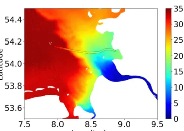
Figure 13.Sea surface salinity on 26 June 2013. Filled contours are model results, and colored lines are observational data from Ferry- Box (FunnyGirl) (Petersen, 2014).
Figure 13 shows the calculated surface salinity field in part of the simulated domain on 26 June 2013 in comparison with the observational data from FerryBox (FunnyGirl) (Petersen, 2014). As can be seen from the plot, there is a high consis- tency of the simulated results with observational data.
6 Discussion
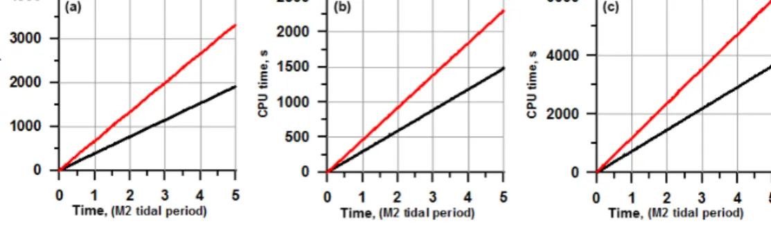
6.1 Triangles vs. quads: numerical performance We examine the computational efficiency by comparing the CPU time needed to simulate five tidal periods of anM2wave on MESH-1 and MESH-2 in the Sylt–Rømø experiment, as presented in Fig. 14. The number of vertices of the quadri- lateral MESH-1 is approximately ∼1.13 that of triangular MESH-2, but the numbers of elements relate as∼0.57. We have found that the total CPU times are in an approximate ratio of 1.62 (triangles/quads). The simulations were per- formed with the same time steps.
The 3-D velocity part takes approximately the same CPU time as the computation of vertically averaged velocity and elevation (external mode). Operations on elements, which in- clude the Coriolis and bottom friction terms as well as com- putations of the gradients of velocity and scalars, are approx- imately twice as cheap on quadrilateral meshes as expected.
Figure 14.CPU time on two meshes, MESH-1 (black line) and MESH-2 (red line), for the Sylt–Rømø experiment. The CPU time for 3-D velocity(a), external mode(b), and the total CPU time(c).
Figure 15.Temperature section along the channel as simulated on the quadrilateral mesh(a). The two inserts show the area adjacent to the open boundary on the purely triangular mesh(a)and the mesh for which the vicinity of the open boundary is rendered with quads(c). The dashed rectangle shows the area of the inserts. Numerical instability evolves on a purely triangular mesh (blue ellipse).
Computations of viscosity and momentum transport are car- ried out in a cycle over edges, which is 1.5 times shorter for meshes made of quadrilateral elements and warrants a sim- ilar gain of ∼1.5 in performance on quadrilateral meshes.
In our simulation, the net gain was∼1.62 times on MESH- 1 compared to MESH-2, despite the fact that the number of vertices is 13 % larger than on MESH-2. The model is stable on the quadrilateral meshes with smaller horizontal viscosity, which is also an advantage.
6.2 Triangles vs. quads: open boundaries
The presence of open boundaries is a distinctive feature of regional models. The implementation of robust algorithms for the open boundary is more complicated on unstructured triangular meshes than on structured quadrilateral meshes.
For example, it is more difficult to cleanly assess the propa- gation of perturbations toward the boundary in this case. In addition, spurious inertial modes can be excited on triangu- lar meshes in the case of the cell-vertex discretization used by us, which in practice leads to additional instabilities in the vicinity of the open boundary. The ability to use hybrid meshes is very helpful in this case. Indeed, even if the mesh is predominantly triangular, the vicinity of the open boundary can be constructed of quadrilateral elements.
We illustrate improvements of the dynamics in the vicinity of the open boundary by simulating baroclinic tidal dynamics in an idealized channel with an underwater sill. The channel
is 12 km in length and 3 km in width, with a maximum depth of 200 m near the open boundary. The sill, with a height of 150 m, is located in the central part of the channel. The flow is forced at the open boundaries by a tide with the period of anM2wave and amplitude of 1 cm, applied in antiphase. The left part of the channel contains denser waters than the right one.
Three meshes were used for these simulations. The first one is a quadrilateral mesh with a horizontal resolution of 200 m refined to 20 m in the vicinity of the underwater sill.
The second one is a purely triangular mesh obtained from the quadrilateral mesh by splitting quads into triangles. The third mesh is predominantly triangular, but for the zones close to the open boundary it is also quadrilateral.
Figure 15 illustrates that at times close to the maximum inflow (8 h 20 m), a strong computational instability due to the interaction between baroclinic and barotropic flow com- ponents evolves on the right open boundary on the triangu- lar mesh, eventually leading to the blowup of the solution (see the left insert). However, by replacing triangles in a small domain adjacent to the open boundary with quadrilat- eral cells we stabilize the numerical solution (see the right insert), which allows us to cleanly handle the directions nor- mal and tangent to the boundary.
7 Conclusions
We described the numerical implementation of the three- dimensional unstructured-mesh model FESOM-C, relying on FESOM2 and intended for coastal simulations. The model is based on a finite-volume cell-vertex discretization and works on hybrid unstructured meshes composed of triangles and quads.
We illustrated the model performance with two test simu- lations.
Sylt–Rømø Bight is a closed Wadden Sea basin charac- terized by a complex morphometry and high tidal activity.
A sensitivity study was carried out to elucidate the depen- dence of simulated surface elevation and horizontal velocity on mesh type and quality. The elevation simulated in zones of wetting and drying may depend on the mesh structure, which may lead to distinctions in the simulated energy on different meshes. The total energy comparison shows that on the tri- angular MESH-2, having approximately the same number of vertices as MESH-1, the solution is more dissipative; higher dissipation is generally needed to stabilize it against spurious inertial modes.
The second experiment deals with the southeastern part of the North Sea. Computation relied on the boundary in- formation from hindcast simulations by the TRIM-NP and realistic atmospheric forcing from NCEP/NCAR. Modeling results agree both qualitatively and quantitatively with obser- vations for the full period of simulation.
Future development of the FESOM-C will include cou- pling with the global FESOM2 (Danilov et al., 2017), the addition of monotonic high-order schemes and sea ice from FESOM2, and various modules that would increase the func- tionality of FESOM-C.
Code and data availability. The version of FESOM-C v.2 used to carry out simulations reported here can be accessed from https://doi.org/10.5281/zenodo.2085177. The General Ocean Tur- bulence Model (GOTM) (Burchard et al., 1999) implemented into the FESOM-C code is published under the GNU Pub- lic License and can be freely used. The meshes are con- structed with the Gmsh software (Geuzaine and Remacle, 2009).
Bathymetry used in the model simulation (Southeast North Sea experiment) is received from the EMODnet Bathymetry Con- sortium (2016) database (https://doi.org/10.12770/c7b53704-999d- 4721-b1a3-04ec60c87238) and is freely available online. The TRIM-NP model is used to initialize runs for 1 year (Weisse et al., 2015). NCEP/NCAR reanalysis atmospheric forcing data (Kalnay et al., 1996) used in the model are freely available online.
Author contributions. AA is the developer of the FESOM-C model with support from VF, IK, and SD. VF, IK, and AA carried out the experiment. AA wrote the paper with support from SD, VF, and IK.
SH and NR carried out the code optimization and parallelization.
KHW and HB contributed with discussions of many preliminary
results. KHW helped supervise the project. All authors discussed the results and commented on the paper at all stages.
Competing interests. The authors declare that they have no conflict of interest.
Acknowledgements. We are grateful to Jens Schröter, Wolfgang Hiller, Peter Lemke, and Thomas Jung for supporting our work.
The article processing charges for this open-access publication were covered by a Research
Centre of the Helmholtz Association.
Edited by: Robert Marsh
Reviewed by: two anonymous referee
References
Androsov, A. A., Klevanny, K. A., Salusti, E. S., and Voltzinger, N.
E.: Open boundary conditions for horizontal 2-D curvilinear-grid long-wave dynamics of a strait, Adv. Water Resour., 18, 267–
276, https://doi.org/10.1016/0309-1708(95)00017-D, 1995.
Barnier, B., Siefridt, L., and Marchesiello, P.: Thermal forcing for a global ocean circulation model using a three-year cli- matology of ECMWF analyses, J. Marine Syst., 6, 363–380, https://doi.org/10.1016/0924-7963(94)00034-9, 1995.
Baschek, B., Schroeder, F., Brix, H., Riethmüller, R., Badewien, T. H., Breitbach, G., Brügge, B., Colijn, F., Doerffer, R., Es- chenbach, C., Friedrich, J., Fischer, P., Garthe, S., Horstmann, J., Krasemann, H., Metfies, K., Merckelbach, L., Ohle, N., Pe- tersen, W., Pröfrock, D., Röttgers, R., Schlüter, M., Schulz, J., Schulz-Stellenfleth, J., Stanev, E., Staneva, J., Winter, C., Wirtz, K., Wollschläger, J., Zielinski, O., and Ziemer, F.: The Coastal Observing System for Northern and Arctic Seas (COSYNA), Ocean Sci., 13, 379–410, https://doi.org/10.5194/os-13-379- 2017, 2017.
Becherer, J., Burchard, H., Floeser, G., Mohrholz, V., and Umlauf, L.: Evidence of tidal straining in well-mixed channel flow from micro-structure observations, Geophys. Res. Lett., 38, L17611, https://doi.org/10.1029/2011GL049005, 2011.
Benjamin, T. B.: Gravity currents and related phenomena, J. Fluid Mech., 31, 209–248, 1968.
Blumberg, A. F. and Mellor, G. L.: A Description of a three-dimensional coastal ocean circulation model, in: Three- dimensional Coastal Ocean Models, edited by: Mooers, C. N.
K., Coast. Est. S., 4, 1–16, 1987.
Burchard, H., Bolding, K., and Ruiz-Villarreal, M.,: GOTM, a gen- eral ocean turbulence model. Theory, implementation and test cases, European Commission, Tech. Rep. EUR 18745 EN, 1999.
Burchard, H. and Bolding, K.: GETM, a general estuarine transport model. Scientific documentation, European Commission, Tech.
Rep. EUR 20253 EN, 2002.
Burchard, H., Flöser, G., Staneva, J. V., Badewien, T. H., and Ri- ethmüller, R.: Impact of Density Gradients on Net Sediment Transport into the Wadden Sea, J. Phys. Oceanogr., 38, 566–587, https://doi.org/10.1175/2007JPO3796.1, 2008.