Research Collection
Doctoral Thesis
Optimization methods for prediction of advanced constitutive models
Author(s):
Hippke, Holger Publication Date:
2020-12
Permanent Link:
https://doi.org/10.3929/ethz-b-000462553
Rights / License:
In Copyright - Non-Commercial Use Permitted
This page was generated automatically upon download from the ETH Zurich Research Collection. For more information please consult the Terms of use.
DISS. ETH NO. 27171
Optimization methods for prediction of advanced constitutive models
A thesis submitted to attain the degree of DOCTOR OF SCIENCES of ETH ZURICH
(Dr. sc. ETH Zurich) presented by
Holger Christian Hippke MSc. ETH, ETH Zurich
born on 22.11.1989 citizen of Germany
accepted on the recommendation of Prof. Dr. P. Hora, examiner Prof. J.-W. Yoon, co-examiner Prof. Dr. D. Mohr, co-examiner
2020
Preface
The present thesis was made possible through research at the Institute of Virtual Manufacturing at ETH Z¨urich during my time as doctoral student.
I would like to thank Prof. Dr. Pavel Hora for his confidence during a large variety of tasks including teaching of major lectures and coordination of industrial projects, as well as for granting me the necessary freedom to conduct research at the institute. With his scientific intuition and guidance, many discussions proved extremely helpful in definition of the work presented.
Many thanks go to Prof. Jeong Whan Yoon and to Prof. Dirk Mohr for inspiring discussions and acceptance of the co-examination.
Further, I want to thank my colleagues at IVP and inspire AG for steady support and great collaborative effort in many projects. Especially the many discussions with Dr. Bekim Berisha are the foundation of profound understanding of the topic at hand. With his great contribution to crystal plasticity, distinct thanks go to Dr. Sebastian Hirsiger, without whom CP would not have been included in this work.
Last but definitely not least, I feel indefinite gratitude to my wife Franziska for unparalleled support, especially in more challenging periods of my doctoral studies.
Contents
Preface III
Abstract VII
Kurzfassung IX
Nomenclature XI
1 Introduction 1
1.1 State of the art . . . 2
1.2 Aim of the thesis . . . 21
2 Analytical investigation and numerical analysis of yielding be- havior 23 2.1 Investigated yield criteria . . . 25
2.2 Reduction of parameter set for with assumptions of isotropic yielding as used in Vegter lite criterion . . . 34
2.3 Analysis of representation space . . . 37
2.4 Investigation of measurement errors on results for plane strain 39 2.5 An interpolation based formulation of yielding for increased flexibility . . . 41
2.6 Conclusion . . . 48
3 Experimental determination of yielding 49 3.1 Strain measurement with DIC . . . 50
3.2 Basic experiments in sheet metal forming . . . 52
3.3 The Nakajima experiment . . . 64
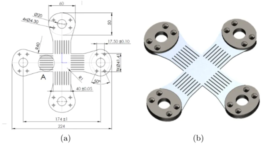
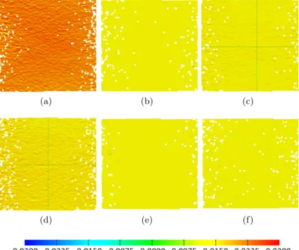
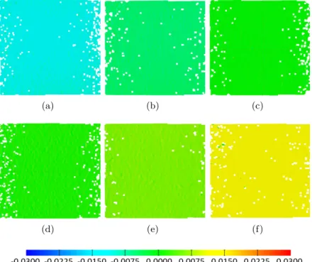
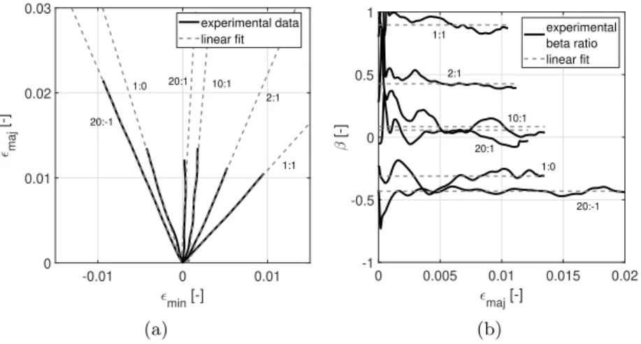
3.4 Initial yield locus with cruciform testing . . . 70
3.5 Initial yield locus based on crystal plasticity calculation . . 81
3.6 Experimentally based definition of yielding . . . 83
3.7 Conclusion of experimental determination . . . 90
4 Inverse full field strain based design of yield surface 91
4.1 Principle of optimization for full-field application . . . 93
4.2 Setup of full field optimization . . . 94
4.3 Application to plane strain with 2D geometry . . . 98
4.4 Sensitivity analysis of YLD2000 parameters using Naka- jima samples . . . 104
4.5 Sensitivity of yield derivative to changes in exponent m for YLD2000 . . . 106
4.6 Optimization of exponent m of YLD2000 using Nakajima samples . . . 109
4.7 Optimization of plane strain point of Vegter using Naka- jima samples . . . 113
4.8 Results and discussion of optimization based yield description114 5 Validation of methodologies 121 5.1 Nakajima cross section test . . . 124
5.2 Validation based on cross-die experiment . . . 134
5.3 Summary of methodologies and optimal result . . . 143
5.4 Conclusion of validation strategies . . . 145
5.5 Cost analysis of all presented methods . . . 147
5.6 Directional testing - common method with a focus on ten- sile loading . . . 149
6 Concluding remarks 153 A Appendix 157 A.1 Derivative of YLD2000 yield criterion . . . 157
A.2 Derivative of Vegter yield criterion . . . 159
A.3 Detailed evaluation of strain error for validation based on Nakajima sections . . . 159
A.4 Sobol indices for non-linear dependency . . . 161
A.5 Dynamic time warping algorithm . . . 161
A.6 Alignment of additional Nakajima samples . . . 163
A.7 Error measures of DTW algorithm of relevant Nakajima geometries . . . 164
Bibliography 167
Abstract
The prediction of strain distribution in production of sheet metal parts di- rectly influences predictions of hardening and failure, as strain and stress response are linked by the yield model. The prediction of strains in sim- ulation is relied upon by tool design and process engineers in all states of development. However, optical measurement and simulation result do not always align, which questions the state of the art approach to define yield models, especially for aluminium alloy. The reason for this mis- match was thought to be the finite complexity of the models used, but while studying the effect, this work shows that not model complexity but an improved foundation for fitting is a solution. Three advanced fitting strategies are presented for non-quadratic and free-shape yield formula- tions. The first is based on macroscopic measurement of cruciform tension specimen as specified in ISO16842 for simultaneous evaluation of strain and stress ratio. The second extracts all necessary information by appli- cation of inverse full field optimization using digital image correlation and global force measurement. The third method investigates the possibility of crystal plasticity calculation based on texture measurement. In order to evaluate performance and to be able to recommend one strategy for fur- ther use, a large validation study is conducted using Nakajima and cross die experiments. Both non-quadratic and free-shape models were able to outperform the original configuration based on the proposed strategies, with cruciform tension and inverse full-field proven to be most effective based on an additional cost analysis. All three strategies provide valu- able information and challenge to reconsider common assumptions about the definition of yielding for aluminium alloy. In consequence, this work presents the basis for further research on optimal choice of fitting strategy, which opens up a new perspective on development of yield models.
Kurzfassung
Die Vorhersage der Dehnungsverteilung bei der Herstellung von Blechteilen beeinflusst direkt die Vorhersage von Verfestigung und Versagen, da die Dehnungs- und Spannungsantwort durch das Fliessmodell verkn¨upft sind.
Die Vorhersage von Dehnungen in der Simulation wird von Werkzeugkon- strukteuren und Prozessingenieuren in allen Entwicklungsstadien herange- zogen. Die Ergebnisse der optischen Messung und Simulation stimmen jedoch nicht immer ¨uberein, was den Stand der Technik bei der Def- inition von Fliessmodellen, insbesondere f¨ur Aluminiumlegierungen, in Frage stellt. Es wurde angenommen, dass der Grund dieses Unterschieds die endliche Komplexit¨at der verwendeten Modelle ist. Bei der Unter- suchung des Effekts zeigt diese Arbeit jedoch, dass nicht die Komplexit¨at des Modells, sondern die experimentelle Grundlage der Modellkalibrierung den Schl¨ussel zur L¨osung des Problems darstellt. Es werden drei erweit- erte Kalibrierungsstrategien f¨ur nicht quadratische und formfreie Fliess- formulierungen vorgestellt. Die erste basiert auf der makroskopischen Messung einer Kreuzzugprobe nach ISO16842 zur gleichzeitigen Bewer- tung des Dehnungs- und Spannungsverh¨altnisses. Die zweite extrahiert alle notwendigen Informationen durch Anwendung inverser Vollfeldopti- mierung unter Verwendung digitaler Bildkorrelation und globaler Kraftmes- sung. Die dritte Methode untersucht die M¨oglichkeit der Berechnung der Kristallplastizit¨at auf der Grundlage einer Texturmessung. Um die Strate- gien zu bewerten und eine davon f¨ur die weitere Verwendung empfehlen zu k¨onnen, wird eine grosse Validierungsstudie mit Nakajima- und Cross-Die- Experimenten durchgef¨uhrt. Sowohl nicht quadratische als auch formfreie Modelle konnten die urspr¨ungliche Konfiguration auf der Grundlage der vorgeschlagenen Strategien ¨ubertreffen, wobei sich die Kreuzzugmethode und die Vollfeldoptimierung aufgrund einer zus¨atzlichen Kostenanalyse als am effektivsten erwiesen. Alle drei Strategien liefern wertvolle Infor- mationen und fordern ein Umdenken grundlegender Annahmen bei der Definition von Fliessmodellen f¨ur Aluminiumlegierungen. Infolgedessen
bildet diese Arbeit die Grundlage f¨ur weitere Forschungen zur optimalen Wahl der Kalibrierungsstrategie, was einen neuen Ansatz f¨ur die Entwick- lung von Fliessmodellen aufzeigt.
Nomenclature
Continuum mechanics
σ stress tensor
strain tensor
W work
ui,j derivative of displacementui with respect toj
F deformation gradient
R orthogonal rotation tensor
E Green-Lagrange strain tensor
S 2nd Piola-Kirchhoff stress tensor σ˙ time derivative of stress tensor
Ω tensor of angular velocity
σ Green-Naghdi stress rate tensor
C elastic stiffness matrix
CEP elasto-plastic stiffness matrix
γ shear strain
Constitutive modelling
Φ yield criterion
F(σij) stress value of yield locus σy stress value of yield curve
Ii invariants of stress tensor, withi∈[1,2,3]
sij deviatoric stress tensor
Ji invariants of deviatoric stress tensor, withi∈[1,2,3]
λ plastic multiplier
Φ0,Φ00 internal parameters of YLD2000 X0,X00 internal parameters of YLD2000 C0,C00 internal parameters of YLD2000 L0,L00 internal parameters of YLD2000 f~ B´ezier part of Vegter yield formulation
A, ~~ B, ~C internal parameters of B´ezier formulation of Vegter Bni(t) Bernstein polynomial, with n: order of polynomial,
i: index of binomial coefficient,t: internal parameter of B´ezier element
b20(t) general parameters of B´ezier curve of second order b0, b1, b2 general parameters of B´ezier curve of second order
~
m, ~n normals on B´ezier element
Nomenclature
β ratio of incremental principal strain
α ratio of principal stress
T stress triaxiality
νL strain based Lode parameter
L stress based Lode parameter
θpolar angle in polar FLC coordinates
κ interpolation parameter of interpolation based YLD2000 F1, F2 internally used yield models in interpolation based
YLD2000 Yielding definition
σtech technical yield stress
tech technical strain
σ true stress
true strain
σeq equivalent stress
eq equivalent plastic strain
F force
A0 initial cross section area
A actual cross section area
L0 initial specimen length
∆L change in specimen length
t specimen thickness
w specimen width
RD rolling direction
DD diagonal direction, 45°to rolling direction TD transverse direction, 90°to rolling direction σi stress value for uniaxial loading, withi∈[0,45,90]
σb stress value for biaxial loading
Ri R-value, strain ratio under tensile loading, with i∈ [0,45,90]
Rb biaxial R-value, strain ratio under biaxial loading F, G, H anisotropy parameters of Hill’48 yield criterion L, M, N anisotropy parameters of Hill’48 yield criterion αi anisotropy parameters of YLD2000 yield criterion
withi∈[1,2,3,4,5,6,7,8]
m exponent of YLD2000 yield criterion
fun,i normalized stress value of Vegter for uniaxial loading withi∈[0,45,90]
fps1,i normalized stress value of Vegter for plane strain in 1st principal direction withi∈[0,45,90]
fps2,i normalized stress value of Vegter for plane strain in 2nd principal direction withi∈[0,45,90]
Nomenclature
fsh,i normalized stress value of Vegter for shear loading withi∈[0,45,90]
fbi normalized stress value of Vegter for biaxial loading Optimization
gi inequality constraints
hj equality constraints
wk weighing factors
¯
i measured true strains
i simulated true strains
F¯j measured global forces
Fj simulated global forces
ASA adaptive simulated annealing General abbreviations
CT cruciform tension
Opt inverse full field optimization YLD2000 intp interpolation based yield locus
YLD2000 var anisotropic yield locus with variable parameter set
CP crystal plasticity
original Yield locus fit as defined in original publication DIC digital image correlation
FE, FEM finite element, finite element method GOM Gesellschaft f¨ur optische Messung
ARAMIS continuous DIC measurement system by GOM ATOS static DIC digitalization system by GOM
LS-Dyna FE software by LSTC
LS-PrePost pre- and postprocessing software by LSTC
MATLAB matrix laboratory, program for evaluation of large numerical data
STL file format of triangular elements
xml ’extensible markup language’, file format for large databases
RVE representative volume element
DAMASK CP-FEM program
EBSD electron back-scatter diffraction
1 Introduction
With Industry 4.0 and the Internet of Things (IoT) shaping the future for an adaptive and connected industry, expectations for computational prediction of real processes are continuously rising. In the last decades, the finite element method (FEM) has become widely applied in industry to provide precise and efficient solutions for complex engineering tasks.
Despite many developments, one topic in discussion remains the method of definition of material behaviour for description of forming processes.
Models with increased complexity are continuously developed to satisfy the demand for extreme precision. However, industrial demand and sci- entific development do not always align. If model complexity is increased by defining more parameters, more experimental testing is needed. Ad- ditionally, many models target only specific scientific challenges and are not necessarily suitable for broad industrial application. The challenge is illustrated in Figure 1.1. An industrial part is shown with many possible failure types. Failure may only be predicted, if incremental strains and stresses are calculated to highest precision during simulation. The calcu- lation of plastic stresses from a given strain field in FEM depends solely on the yield locus, a function defining the boundary between elastic and plastic loading. The yield locus will be the focus of this work as it is a center piece in prediction of yielding.
Several advanced methods to define precise models are presented, while being constantly aware to minimize experimental effort. In order to eval- uate these methods, they are compared with industrial standards with regard to precision and applicability. Model performance is validated on both a standardized experiment and an industrial demonstrator part.
Figure 1.1: The central challenge: stress and strain distribution need to be predicted correctly to reduce failure in production. This may only be achieved by correct prediction of yielding. Figure combined from [54, 62, 61, 60].
1.1 State of the art
Due to the high complexity of industrial geometries, the demand for pre- cision of digital prediction is continuously rising. This section familiarizes the reader with the current state of research and gives insight in the historical development of constitutive modelling. A short outline of the industrial process is given in Section 1.1.1, followed by a repetition of con- tinuum mechanics for large strains in Section 1.1.2. Considerable detail is provided on the field of constitutive modelling in Section 1.1.3, followed by an introduction to plastic yielding in Section 1.1.4. A special focus lies on yield criteria, with anisotropic and non-quadratic models described in Section 1.1.5 and 1.1.6 and free shape models in Section 1.1.7. Section 1.1.8 focuses on the experimental basis and more advanced approaches are discussed in Section 1.1.9.
1.1 State of the art
1.1.1 Metal forming
Figure 1.2: From crystal structure to rolling texture and finally anisotropy.
Illustration of material description on different scales. EBSD map from [88].
The structure of metals on an atomic basis in an optimal case is in the form of crystals. Three major types of metal crystals exist: body centered cubic (BCC) in ferritic steels, face centered cubic (FCC) in e.g. aluminium and copper and hexagonal close-packed (HCP) in e.g. titanium. These crystal structures are only ideal in theory. Missing atoms within the struc- ture, called dislocations, or atoms of other materials, called interstitials, exist within a metal’s crystal grid. These small errors significantly influ- ence the metals formability, with dislocations in favor of deformation and interstitials hemming deformation. In addition, the structure of metallic crystals is strongly influenced by deformation during production, such as the rolling of sheet metal. This introduces macroscopic differences of the material in dependency of the angle to rolling direction (RD), which is easiest displayed by tensile measurements in different directions. In con- sequence, it becomes necessary to describe any sheet metal in dependency of the angle to rolling direction. This is commonly achieved by the use of anisotropic yield models, which map a different stress response in depen- dency of the angle to RD.
The dominating production process using flat sheet is the deep drawing process, as illustrated in Figure 1.3. In principle, a piece of sheet metal is held by blank holder and die and a punch in the shape of the final work piece is pressed into the metal, deforming it into its final shape. This
process may be repeated with different punch shapes for more complex geometries. A very detailed description of forming processes is given by Lange [93], Banabic [30] and others [34, 86]. Today, the three major fields in prediction of processes are characterizing process parameters, defining computation with finite element (FE) and describing material behavior.
The challenges in process design are explained and summarized by Lange [93] and Doege and Behrens [34].
In contrast to the process side, the computation and prediction of pro- cesses is a relatively new field, with first industrial application inspired by a VDI benchmark in 1991 [41], that asked to predict strain distributions on a complex forming geometry. This gave rise to popularity and applica- bility of special purpose FE programs such as Autoform and established the explicit FE formulation for commercial purposes. Extended details of the computational representation of processes are given by Hartley [55]
and Dunne and Petrinic [40] with elaborate details on the FE method by Bathe [11]. The description of the material response is the field of study of this work and will be presented in detail in the following sections.
Figure 1.3: Principle of deep drawing by [86].
1.1 State of the art
1.1.2 Continuum mechanics for forming processes
This section introduces stress and strain measures common for engineer- ing applications. If a body undergoes a change of shape without change of position or rotation, we strive to describe this change of shape, or defor- mation, with the strain tensor. The basics of continuum mechanics teach, that the formulation of the strain tensor for small deformation is given as ij = 1/2(ui,j+uj,i). While this formulation holds for most applications, large plastic deformation and rotation require an extended formulation in- cluding either higher order terms as given in Equation (1.2) or a separate treatment of rotation as is common in FEM. A short description of the underlying basics of continuum mechanics is presented by ¨Ochsner [157].
The underlying principle is, that the stress integrated over the strain must be equal to the work required, see Equation (1.1).
W = Z
σd (1.1)
A pair of strains and stresses that satisfy this condition is called a work conjugate pair. The corresponding work conjugate strain to the true stress σ=F/A, also Cauchy stress, is the true strain, or Hencky strain, defined as=ln(L/L0). This pair is commonly used in incrementally integrated FE applications for large strains. An additional requirement for forming applications fulfilled by this pair are objective strain and stress measures, meaning measures independent of coordinate systems. However, the con- tinuum mechanics for large strain applications include more advanced formulations.
ij= 1
2[ui,j+uj,i+uk,iuk,j] (1.2) In order to introduce common formulations in continuum mechanics, the deformation gradient F is introduced as the derivative of the current positionxwith respect to the previous positionX, as given in Equation (1.3).
F = ∂x
∂X (1.3)
This formulation enables us to write the strain measure of Equation 1.2 equivalently as
E= 1
2(FTF −I) (1.4)
called the Green-Lagrange strain tensor [40]. Ottosen and Ristinmaa [107]
efficiently illustrate that this tensor describes the desired deformation without rigid body motion and independent of the coordinate system.
E is not work conjugate to Cauchy stress, but to the 2nd Piola-Kirchhoff stressS, defined in Equation (1.5).
S =det(F)F−1σF−T (1.5) This formulation becomes important in the Total-Lagrangian formulation for large strain in continuum mechanics and special FE applications. In the incremental Updated-Lagrange formulation, such as the elasto-plastic material integration, the rate of stress is computed. However, the Cauchy stress rate is not objective. As a result, various objective stress rates have been introduced by Jaumann, Truesdell (1965) [137] and Green-Naghdi (1965) [48]. The Geen-Naghdi stress rate is given in Equation 1.6 as an example, using the angular velocity Ω= ˙R·RT. A detail description of the FE formulation is found by Belytschko (2014) [12].
σ= ˙σ+σ·Ω−Ω·σ (1.6) As the explicit dynamic FE application used in this work integrates small increments of strains and stresses in a co-rotational coordinate system, the Cauchy stress and Hencky strain formulation is used for most cases.
Having introduced stress and strain measures, a reminder is given to their inter-dependency, which is referred to as constitutive equations. For uni- axial elastic deformation, Hooke’s law σ = E is sufficient. Which is extended to the three dimensional case by defining the Poisson’s ratio as ν =−yy/xx. The Young’s modulusEis replaced by the elastic stiffness matrixC.
σ=C· (1.7)
When symmetry conditions are considered this is reduced to the form
σxx
σyy
σzz σxy σyz σxz
=(1+ν)(1−2ν)E
1−ν ν ν 0 0 0
ν 1−ν ν 0 0 0
ν ν 1−ν 0 0 0
0 0 0 1−2ν2 0 0
0 0 0 0 1−2ν2 0
0 0 0 0 0 1−2ν2
xx
yy
zz γxy γyz γxz
(1.8)
1.1 State of the art
For implicit quasi-static FE application, the incremental deformation in- creases and an extended elasto pastic stiffness matrix CEP needs to be derived, as described in Section 1.1.4.
1.1.3 Constitutive modelling and isotropic yield criteria
Constitutive modelling is the science to describe macroscopic physical be- havior of materials in mathematical form. The most basic form of a con- stitutive model is to assume rigid behavior until a cutoff value is reached, commonly the yield strengthRp02. An only slightly more complex formu- lation is to follow Hooke’s law until the cutoff valueRp02is reached. This form finds a large array of application in layout and design of mechanical parts in engineering and is the basis for the whole field of dimensioning.
As this work strives to improve predictions of forming processes, the plas- tic range after Rp02 becomes of central importance. Material behavior becomes non-linear, requiring more sophisticated models. For a uniaxial stress state, as is commonly determined in tensile condition, a function is derived describing the uniaxial stressσy in function of equivalent plas- tic strain eq. The result of the underlying uniaxial tensile experiment is displayed in Figure 1.4, illustrating the elastic and plastic zones and both engineering and true strain and stress. Depending on the shape of the measured progression, a large variety of models have been suggested by Swift [131], Voce [146], Gosh or Hockett-Sherby [66] or others. Ad- ditions for rate and temperature dependency are presented by Cowper and Symonds [29] and Johnson and Cook [83] and a formulation includ- ing austenite-martensite micro structure of stainless steels is available by H¨ansel [74]. Despite the increasing complexity, these models do not yet describe the multi dimensional stress states found in common forming ap- plications.
The measurement of stress states under multi dimensional loading be- comes more cumbersome experimentally and assumptions are made to describe general loading cases. To give an overview, the most simplified case is assumed first. An isotropic material is considered, referring to a material with equal resistance to plastic deformation independent of load- ing direction. Additionally, only proportional loading, rate independence and isotropic hardening is considered. Under this set of assumptions, a
Figure 1.4: Representation of both an engineering and a true uniaxial stress-strain curve translated from [34].
criterion is sought, that describes the onset of plastic yielding. As other influences are excluded, the criterion is only a function of stress state:
Φ =F(σij)−σy ≤0 (1.9)
This criterion is referred to as yield criterion. The investigation of yield criteria is the focus of this work. Criteria that fulfill condition 1.9 are developed and presented since the Tresca yield criterion has been formu- lated in 1864 [136]. In consequence the following introduction to the field is not exhaustive with regard to existing criteria, but merely an overview of criteria with significance to simulation of sheet metal forming processes.
AsF is generally a function of the stress tensor, early criteria are formu- lated in dependency of invariants Ii of the stress tensor, which are given in index notation as
I1=σii (1.10)
I2= 1/2σijσij (1.11)
I3= 1/3σijσjkσkl. (1.12) With the additional assumption of constant volume, or pressure indepen- dency as discussed by Spitzig and Richmond [126, 125] and Casey and Sullivan [22], it is more advantageous to use invariants of the deviatoric
1.1 State of the art
stress tensor sij = σij −1/3δijσkk. Deviatoric stresses are defined as the remaining stresses after substraction of hydrostatic pressure. In the case of isotropic hardening, only deviatoric stresses take part in plastic deformation. The resulting set of relevant invariants becomes
J1=sii = 0 (1.13)
J2= 1/2sijsij (1.14)
J3= 1/3sijsjkskl =s1s2s3 (1.15) asI1directly represents the hydrostatic stress, the general yield criterion becomes
F(J2, J3)−σy= 0 (1.16) withJ2 andJ3describing the influence of deviatoric stress. Additionally, for many metals it is assumed that the criterion is symmetric with respect to the stress state, meaning that the loading states σij and −σij return the same result. Based on this set of assumptions, von Mises defined a yield criterion for ductile metals in 1913 [101] based onJ2:
p3J2−σy = 0 (1.17)
With the factor of 3 due to the solution of the yield criterion for uniaxial tension as √
3J2 =σy, which is interpreted as equivalent work necessary to deform a body independently of stress state using the tensile condition as reference.
1.1.4 Plastic yielding - the associated flow rule
Von Mises [102] wrote in 1928, that the principle stress directions must be equivalent to the principle strain rate directions and that the magni- tude of both only differs by a constant. This thought was extended when Drucker [35, 37] formulated the associated flow rule (AFR) in 1950 based on the thermodynamic principle of maximum generated entropy. As the flow rule is of central importance in this work, the principle is explained in more detail.
The yield criteria F described in Section 1.1.3 define the boundary be- tween elastic and plastic stress states and as such are a function of the
stress tensorσij only. The relation between stress and strain for the uni- axial case was explained in Section 1.1.2 and is illustrated as yield curve in Figure 1.4. So far, this excluded general stress states.
Assuming additive decomposition of the general strain increment dtot, Equation 1.18 holds.
dtot=del+dpl (1.18)
Based on the elastic relation given in Equation 1.8,del is known for gen- eral cases asdelij =Cijkl−1dσkl.
To derive the plastic strain increment, the assumption is that any incre- ment of plastic strain requires a certain amount of plastic work, as defined in Equation 1.19.
dWpl= ∆σij·dplij >0 (1.19) If Equation 1.19 must hold irrespective of the stress state, dWpl = 0 may only hold if the stress points moves on the yield surface and thus no plastic work is required. In consequence, the plastic strain increment must be perpendicular to the stress increment. In other words, the plastic strain increment is proportional to the derivative of the yield surface.
Equivalently, it may be stated that a plastic potential exists, which is equivalent to the yield surface. This formulation is referred to as the associated flow rule (AFR) [15, 129], introducing the plastic multiplierλ as scaling factor.
dplij =λ· ∂F
∂σij (1.20)
An associated uniqueness theorem is provided by Hill [57] and extended to a derivation from single crystals by Bishop and Hill [14]. Drucker [38, 39] established an extended stability criterion using associated flow.
The stability criteria were later extended by Stoughton [129] for use with non-associated flow rule.
With this information, we are able to formulate the elasto plastic material law as
dσij =Cijkl
dtotkl −λ∂F
∂σij
(1.21) It shall now be considered that after plastic deformation the yield locus expands and the new stress state must be on the expanded yield locus.
This condition in Equation 1.22 is referred to as consistency condition
1.1 State of the art
[11, 40], based on the first order terms of a Taylor series.
∂F
∂σij
dσij− ∂σy
∂eq
deq = 0 (1.22)
If combined with Equation 1.9 and Equation 1.20 it may be reformed to return a solution for λand for the elasto-plastic material modulus as relation of strains to stresses for general cases in Equation 1.24. This formulation is of central importance in implicit FE calculation.
λ=
∂F
∂σijCijkldtotkl
dσy
deq +∂σ∂F
ijCijkl ∂F
∂σkl
(1.23)
dσij =Cijkl 1−
∂F
∂σijCijkl ∂F
∂σkl dσy
deq +∂σ∂F
ijCijkl∂σ∂F
kl
!
dkl (1.24)
A similar approach is used to derive an increment of λ, which is com- monly implemented in explicit material integration and which is given in Equation (1.25).
dλ= F−σy
dσy deq +∂σ∂F
ijCijkl ∂F
∂σkl
(1.25) The total effective plastic strain increment is calculated by integratingdλ.
1.1.5 Anisotropic yield criteria
For application in sheet metal forming, planar anisotropy is illustrated by drawing a circular blank into a cup shape. The experiment suggests to reduce the set of assumptions made in Section 1.1.3 to allow for anisotropic yielding. Due to the rolling of sheet metal, the microstructure develops a distinct texture and becomes dependent on the rolling direction, as described by Ostermann [106] and Banabic [30] and others [63]. The cup drawing experiment was discussed as early as 1948 by Hill [56] and is still widely in use today for the purpose of validation [134, 156, 62]. Banabic [3] provides a well structured overview of available anisotropic models, which is in part given in Table 1.1. An early criterion defined by Hill
Yield model σ0 σ45 σ90 σb R0 R45 R90 Rb σ15i R15i σP S σSH
Hill’s family
Hill 1948 x x x x
Hill 1979 x x x
Hill 1993 x x x x x
Lin, Ding 1996 x x x x x x
Leacock 2006 x x x x x
Hershey’s family
Hosford 1979 x x x
Barlat 1991 x x x x
Karafillis Boyce 1993 x x x x x x
BBC 2000 x x x x x x x x
Barlat Yoon 2000 x x x x x x x x
Barlat 2004 x x x x x x x x x
Drucker‘s family
Cazacu-Barlat 2003 x x x x x x x x x x
C-P-B 2006 x x x x x x x x x x
Polynomial criteria
Comsa 2006 x x x x x x x x
Soare 2007 (Poly 4) x x x x x x x x x x Hu 2020 (Poly4*Hosford) x x x x x x x x x x Free shape criteria
Vegter 2006 x x x x x x x x x x
Vegter lite 2009 x x x x x x x x
Raemy 2017 (FAY) x x x x x x x x x x x x
Hao Dong 2020 x x x x x x x x x x x x
Table 1.1: A selection of anisotropic yield models and mechanical param- eters needed as structed by Banabic [3]. Minor extensions are included for free-shape and polynomial yield models.
1.1 State of the art
[56, 57] is based on the assumption that anisotropy may be defined by a fourth order tensor P such that
sijPijklskl−1 = 0. (1.26) As illustrated in consise form in [108] this formulation is easily transformed to the von Mises yield criterion and, when assumptions of symmetry and orthotropy are taken into account,P becomes
P =
F+G −F −G 0 0 0
−F F+G −H 0 0 0
−G −H G+H 0 0 0
0 0 0 2L 0 0
0 0 0 0 2M 0
0 0 0 0 0 2N
(1.27)
And Equation 1.26 becomes the Hill’48 yield criterion withF, G, H, L, M, N as material constants describing anisotropy. Similar adaptions are made by Hosford and Backofen [70] and a more generalized form by Hill [58].
Further additions without assumption of symmetry are made by Tsai and Wu [138], which is a reduction of the Hoffman criterion [67]. Another mathematical approach with similar result was pursued by Dafalias and Rashid [31]. The entire set of criteria discussed so far are quadratic in terms of stresses. However, not every measurement is represented well with quadratic forms, especially for measurements of aluminium alloys.
This leads to the additional families of non-quadratic and free shape yield criteria, which will be introduced in Section 1.1.6 and 1.1.7.
WhileJ2based yield criteria are considered sufficient for orthotropic and symmetric yielding, extensions to include the third invariant of the devi- atoric stress tensorJ3have been discussed early on by Drucker [36], with a generalization by Cazacu and Barlat [23] and an extension to general three dimensional form presented by Yoshida et al. [152]. Gao et al. [44]
additionally included I1. Yoon et al. [151] presented a model in func- tion of all three stress invariants specifically tailored to pressure sensitive metals, with an extension as a ductile fracture criterion [96].
1.1.6 Non-quadratic anisotropic yield criteria
A detailed description of linear transformation based yield criteria is given by Barlat, Yoon and Cazacu in [10]. An early Yield criterion of higher order has been introduced by Barlat and Lian in 1989 [9]. The underlying concept is similar to the formulation of quadratic yield criteria. Yielding is described for incompressible, symmetric and orthotropic materials by defining a yield criterion based on deviatoric stress invariants and applying a number of linear transformations. Energy equivalence must hold for all states on the yield surface, which is automatically fulfilled if linear transformations are applied to the stress tensor. A single transformation
˜
sis described in agreement with Equation 1.26 as
˜
s=Cijklsij (1.28)
This form was applied by Barlat’s six component yield function [8] with additions made by Karafillis and Boyce in 1993 [84] for face centered cubic (FCC) materials and body centered cubic (BCC) materials. To increase complexity and the amount of anisotropy parameters, the transformation may be applied an infinite number of n times. Bron and Besson [17]
and Barlat et al. (2005) [5] applied two linear transformations for general stress states, which results in a total of 18 parameters. Barlat et al. (2003) [6] applied two linear transformations for plane stress which returns eight anisotropy parametersαi. The exponentmof the model is recommended to be m = 6 for BCC and m = 8 for FCC materials based on research by Logan et al. [95]. The resulting model is commonly referred to as the YLD2000 model and will be used extensively in this work, as it represents the state-of-the-art in the aluminium industry. To illustrate the effect of the parameters, two special cases are considered, as suggested by Barlat et al. [10]. The first considers the shear stress to be zero and the second considers the normal stresses to be zero:
F =|α1sxx−α2syy|a+|α3sxx+ 2α4syy|a+|2α5sxx+α6syy|a (1.29) F =|2α7sxy|a+ 2|α8sxy|a
All details of the model will be described in Section 2.1.1. The imple- mentation of the model into FE code is described by Yoon et al. [150].
A recent update of the family of criteria has been provided by Aretz and
1.1 State of the art
Barlat [1] with up to 27 parameters.
Criteria with a very large set of parameters pose a challenge for industrial applicability due to the amount of necessary testing. Van den Boogaard et al. [16] and later Lou et al. [97] reduced the parameter set for defor- mation of metals of the YLD2000-18p model, increasing its applicability.
Modelling of anisotropic and kinematic hardening
As the original assumptions are reduced, more and more detailed and complex constitutive models are defined. Differences in tension and com- pression and kinematic hardening are included by Yoshida and Uemori [153], in the Homogeneous-Anisotropic-Hardening (HAH) model [7] and in a model by Chun et al. [25]. Anisotropic hardening without kinematic effects may also be described by considering a plastic strain dependency of the parameter set of any yield locus, as presented by Wang et al. [148] or in different form by Peters et al. [112] on the example of the YLD2000 cri- terion. Asymmetric yielding, especially in use for hexagonal close packed (HCP) materials has been presented by Cazacu et al. [24] and tested by Baral et al. [4].
1.1.7 Free shape yield criteria
Using a less physically motivated approach, a yield criterion is a convex and continuous surface that is at least once continuously differentiable.
Many mathematical formulations are possible. In order to describe com- plex anisotropic behavior, a large number of degrees of freedom is sought for. To allow for an increased variability in modelling, Vegter et al. [142]
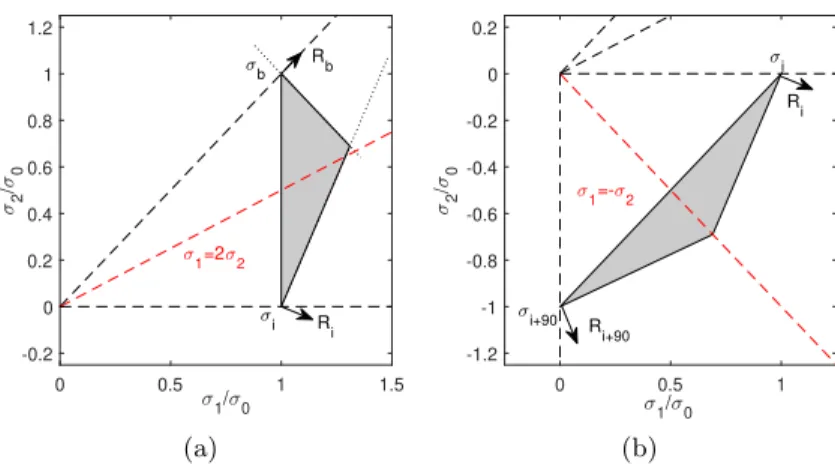
suggested an approach based on a combination of B´ezier and Fourier in- terpolation in 1995, which was extended to planar anisotropy by Carleer et al. [21]. Pijlman et al. [113] further presented the details for implemen- tation and the model found increasing interest in 2006 [145]. WhileF was previously defined as a function of the stress tensor σij or the deviatoric stress tensor sij, the Vegter yield criterion describes the yield function F in dependency of principle stresses σ1 and σ2 under the assumption
Figure 1.5: Reference and hinge points of the Vegter model [21]
of plane stress. To construct a continuous yield criterion, second order B´ezier elements are linked, using four reference points at the conditions of uniaxial tension, equibaxial tension, plane strain and shear. The hinge points are calculated as intersections defined by the derivative in the ref- erence points, as illustrated in Figure 1.5. The choice of B´ezier elements ensures a convex and continuously differentiable yield criterion. This de- fines a yield criterion for planar anisotropy, which is easily extended to asymmetric yielding with great variability in the adjustment of process relevant stress states, such as the plane strain state. The Vegter yield cri- terion has become widely available with implementations in commercial FE codes. In order to reduce the complexitiy, simplifications and adjust- ments have been published, such as the Vegter lite model [143, 144]. A very similar approach was recently published by Hao and Dong [53].
An additional free shape yield criterion has been published by Raemy et al. (2017) [117], referred to as FAY (Fourier Asymmetric Yield) model.
The FAY model selects Fourier series instead of the B´ezier interpolation of the Vegter criterion, allowing for an additional increase in flexibility at the risk of non-convexity, as Fourier series require an additional check of convexity. If used with the necessary care, the FAY model has found great applicability in titanium alloys [116], as it covers both asymmetry and planar anisotropy.
A different strategy with similar results was pursued by Comsa and Ban-
1.1 State of the art
abic [26] and Soare et al. [122] and later by Hu et al. [72], using higher order polynomials to fit measured yield data. The resulting yield crite- ria are very adjustable and thus comparable with the Vegter and FAY criterion.
1.1.8 Experimental determination of yield criteria
0 20 40 60 80
0.75 0.8 0.85 0.9 0.95 1
/0
experimental data advanced modeling standard YLD2000
(a)
0 20 40 60 80
degree to RD 0.2
0.4 0.6 0.8 1 1.2 1.4 1.6
R
(b)
Figure 1.6: Strategy to fit complex yield models based on tensile experi- ments every 15 degrees to rolling direction on the example of an AA2090 aluminium alloy [109].
Experimental testing is conducted to determine stresses for predefined load cases,σij(ij(t)). While isotropic models [101, 136] rely entirely on one uniaxial tensile test [81], anisotropic models introduced the need for additional testing. The first strategy was to use the direction dependency of the material and to repeat the uniaxial test in other in-plane directions as suggested by [56] for rolling direction (RD), transverse direction (TD) and diagonal direction (DD). Every tensile test returns both the uniaxial stress and the corresponding derivative in form of R-value, or Lankford parameter. For more complex models such as the YLD2000 [6], a measure- ment of biaxial stress and biaxial R-value is suggested. Todays standard
tensile & bulge
special tensile tests
in-plane torsion tube expansion cruciform
shear
mini punch
Figure 1.7: Experiments in use for definition of initial yielding of sheet metal. Details of experiments are found in [79, 81, 92, 119, 103, 149].
for biaxial stress is the bulge experiment [79]. Measurement of the biaxial R-value is obtained by disc compression test, as suggested by [6]. In to- tal, tensile testing in three directions and biaxial testing returns sufficient information for 8 parameters. A regularly observed practice is to increase the amount of data used for parameter determination by increasing the amount of tensile tests to one test every 15 degrees to rolling direction [109]. This set of data investigates only one stress state but returns a suitable set of data to fit more complex models and is displayed in Figure 1.6. A different approach is persued by Vegter et al. [145] by defining both dedicated plane strain and shear testing designs to obtain additional datapoints. Roth and Mohr [119, 120] have provided a systematic analy- sis of the design of advanced tensile and shear specimen and Lenzen and Merklein have discussed an adjusted bulge experiment for plane strain in [94].
Kuwabara et al. [91, 80] have realized the need for a larger experimental basis early on by proposing a cruciform testing setup. Alternatives are dis- cussed by Hannon and Tiernan [52]. Geiger et al. [45, 73] and Tasan et al.
[132] have provided similar alternative experimental methods. Cruciform testing provides an opportunity to define loading in two perpendicular axis directions. Digital image correlation (DIC) provides information on local displacement. As the specimen geometry is critical for homogeneous
1.1 State of the art
Figure 1.8: Illustration of critical loading state in plane strain in FLD and stress space. Standard measurements often neglect the importance, as is shown on the example of tension and biaxial loading.
distribution of strains within the specimen, the topic has been widely discussed [32, 140]. Hou et al. [71] have designed a cruciform specimen for large strains specifically for dual-phase steels. Upadhyay et al. [140]
provide an overview. The line of thought was extended to tube expan- sion by Kuwabara [89] and Kuwabara and Sugawara [92], with a tube formed by internal pressure and additional axial stresses. An extended tube testing approach, called Ring Hoop Tension Test, was presented by Dick and Korkolis [33]. All of these testing methods provide informa- tion on material response in plane strain state, as it represents the most critical loading case under plane stress. The correlation between critical states in the forming limit diagram (FLD) and stress space are illustrated in Figure 1.8. Another testing method, known as the In-Plane Torsion Test, focuses on shear loading and has been investigated by Tekkaya et al.
[133, 135] for the description of anisotropic yielding. Grolleau et al. [49]
have presented a similar testing geometry for determination of anisotropy.
1.1.9 Advanced approaches
Previous sections introduced the most commonly used assumptions, ex- periments and models. Within the last years, these assumptions have
been questioned and very recently, in parallel with the presented work, new strategies for the determination of yield criteria have evolved.
By measuring pressure sensitivity and determining a volume expansion considerably smaller than predicted with AFR, Spritzig et al. (1975) [126]
suggested, that AFR does not hold in all cases. This experimental finding sparked extensive research and is the foundation to use non-associated flow rule (nonAFR) for metals. Casey and Sullivan [22], Brunig [18] and Stoughton and Yoon [128] came to the conclusion, that pressure sensitiv- ity is prediced correctly when using nonAFR. Stoughton and Yoon [129]
further established a set a stability conditions for nonAFR in 2006. Safaei et al. [121] investigated the implementation of nonAFR and introducted a scaling factor to ensure that yield locus and plastic potential intersect at uniaxial tension. Investigations using nonAFR have been conducted by Park and Chung [109] and Hippke et al. [62] and others. While nonAFR finds increasing application in scientific scenarios, industrial applications are rare, as the increased set of parameters introduces higher risk of over- fitting.
Recently, a discussion of suitable exponents of non-quadratic yield mod- els for BCC and FCC metals has evolved, based on research presented by Manopulo et al. [99], Hippke et al. [61] and Pilthammer et al. [114]. All authors have found strong indication, that the long standing assumption of an exponent 6 for BCC and an exponent 8 for FCC metals may not be true.
In the field of parameter identification, microstructural analysis from the field of material science has found increased application in constitutive modelling. Roters et al. [118] provided a crystal plasticity (CP) FFT program and Hirsiger et al. [64] and Coppieters et al. [28] presented ap- plicable stategies in 2018 both using large amounts of scientific computing power. More applications in the field followed by Berisha et al. [13] and Han et al. [51] and it remains an active scientific field.
Another very recent approach for evaluation of parameter sets for yield criteria has evolved though mathematical optimization strategies. G¨uner et al. [50] have presented a first approach for inverse identification of yield loci using optically measured strain fields. Ilg et al. [75, 76] outlined the possibilities of the commerical optimizer LS-Opt using optically measured tensile experiments and Coppieters et al. [27] recently extended the ap- proach to a cruciform specimen with increased complexity.
1.2 Aim of the thesis
Figure 1.9: Full-field optimization strategy used by Ilg et al. [75] to fit post necking regime of tensile experiments.
1.2 Aim of the thesis
With the amount of research documented, it becomes clear that the scien- tific field of constitutive modelling is continuously searching for increased precision in both experiments and models in every possible direction.
The description of plastic material behaviour remains challenging, as the requirements for manufacturing design include extreme precision, while small measurement errors suffice to significantly change resulting models.
The gap between industrial application and research focus is increased, as the many options are rarely compared to real production. Increasing the understanding of constitutive modelling and defining a suitable approach for industry is the aim of this work. Correct prediction of plane strain loading presents a central challenge, as it represents the most critical stress state in sheet metal forming. As the YLD2000 and the Vegter model rep- resent the current industrial standard in modelling of aluminium alloys, these two models will be combined with the described advanced methods.
Performance in dependency of modeling strategy is measured on the basis of Nakajima and cross die testing. The content may be summarized in the following points:
• pursue advanced experimental strategies for determination of constitu- tive models,
• exploit mathematical optimization schemes to increase model precision,
• analyze sensitivity of constitutive models for FE applications,
• focus on prediction of plane strain loading,
• use an industrial geometry to define suitable long term strategy,
• quantify model performance using an industrial demonstrator,
• highlight optimal strategies for industrial application.
2 Analytical investigation and numerical analysis of yielding behavior
A large number of yield formulations has been introduced in Chapter 1, ranging from isotropic yielding with von Mises [101] and Tresca [136] to anisotropic yielding with Hill’48 [56], YLD2000 [6] and free shape criteria such as Vegter [145] and FAY [117]. Additionally, anisotropic and kine- matic hardening, such as YLD2000var [112], HAH [7] and Yoshida model [152] are introduced. This large set of models needs to be reduced to a sub- set of industrially applicable cases. The two metals most commonly in use in sheet metal forming are deep drawing steels (DC) and aluminium 6000 and 7000 alloys. Deep drawing steel has been used in automotive indus- try for many decades, with modeling using Hill’48 or recently YLD2000.
Aluminium has found introduction in series production as a lightweight alternative to steel for non-structural components and is most commonly modeled by YLD2000 or recently Vegter type yield formulations. Figure 2.1 illustrates yield locus shapes for DC05 steel and 6014 aluminium. The largest apparent difference is a focus on biaxial influence for steel. This introduces a well defined plane strain point and continuously changing derivatives. Aluminium exhibits a strongly plane strain dependent yield behavior due to only minor differences in yield normal, which explains difficulty to predict the response of aluminium in plane strain. Many steels are both strain rate dependent and exhibit anisotropic hardening, which reduces the significance of statements focused on yielding alone due to interaction of effects. For aluminium alloys these effects are negligible allowing for a clean investigation of yield locus influence. As development leans towards more flexible formulations, YLD2000 and Vegter are chosen to be investigated on the example of a 6014 aluminium alloy. The exper- imental and optimization based methods are equally applicable to steel, when anisotropic hardening and rate sensitivity are taken into account.
In order to investigate the influence of YLD2000 and Vegter for applica-
-0.5 0 0.5 1 1.5 xx/ 0
-0.5 0 0.5 1 1.5
yy/0
Steel YLD2000 Steel Hill48
(a)
-0.5 0 0.5 1 1.5
xx/ 0 -0.5
0 0.5 1 1.5
yy/0
Aluminium YLD2000 Aluminium Vegter
(b)
Figure 2.1: Typical yield shapes for DC05 deep drawing steel in (a), show- ing Hill48 based on R-values and YLD2000. Original data from [111]. Equivalently typical shapes for aluminium 6014 in (b), with YLD2000 and Vegter. The large difference in plane strain and biaxial yielding is apparent.
2.1 Investigated yield criteria
bility in FEM and industry, it is of central importance to be familiar with the respective formulations, as given in Section 2.1. In addition, further details are needed to understand the mechanism of the Vegter model and Section 2.2 investigates an option to reduce the input data by making an assumption derived from isoptropic yielding. As the two yield criteria are defined in dependency of different variables, Section 2.3 illustrates valid transformations between different variables in stress and strain space. A short discussion of common and advanced representation spaces and their advantages is the topic of Section 2.3.1. Important influences of mea- surement of plane strain point are presented in Section 2.4 and a novel modelling approach based on interpolation of two YLD2000 yield loci is found in Section 2.5. Section 2.6 summarizes the content of the chap- ter.While the analytical sensitivities represent the response of the model to a parameter change, this change is better investigated for a specific geometry. In consequence, a sensitivity analysis is part of an optimization of Nakajima geometries and is presented in Section 4.4.
2.1 Investigated yield criteria
Two families of yield criteria will be discussed in this work. The first are non-quadratic linear transformation based criteria, with the example of YLD2000, and the second are geometrical formulations based on interpo- lation functions, with the example of the Vegter criterion. Both models will be introduced. Stability conditions will be derived for both plane strain and shear condition for the Vegter criterion, as the geometrical definition leaves room for non-convex solutions.
2.1.1 The YLD2000 yield criterion for plane stress
The YLD2000 formulation is a non-quadratic yield locus for plane stress condition proposed by Barlat et al.(2003) [6]. It accounts for planar anisotropy and higher order flow exponents. The formulation is based on eight parameters αi for anisotropy and an exponentm. This section introduces the model formulation, with details on the derivatives given in Appendix A.1. The yield surface is a function of general stress state
[σx, σy, τxy]. The formulation for the yield locus uses two linear transfor- mations on the stress tensor:
2¯σy= Φ0+ Φ00 with
Φ0=|X10 −X20|m , Φ00=|2X200+X100|m+|2X100+X200|m with
X1=f1(αi,σσσ) andX2=f2(αi,σσσ)
(2.1)
X10 and X20 are the principal values ofXXX0. The same applies toX100 and X200. The transformed stress tensorsXXX0 andXXX00are defined as
X
XX0=CCC0TTT σσσ=LLL0σσσ XXX00=CCC00TTT σσσ=LLL00σσσ
Where CCC0, CCC00, TTT represent the transformation matrices for two linear transformations of the stress tensor σσσ. Please note, if CCC0 and CCC00 are equal to the unit matrix, the yield function becomes isotropic. The two linear transformations are combined in the tensorsLLL0 andLLL00, which are given below as function of the anisotropy parametersαi.
LLL0= 1 3
2α1 −α1 0
−α2 2α2 0
0 0 α7
LL L00= 1
9
8α5−2α3−2α6+ 2α4 4α6−4α4−4α5+α3 0 4α3−4α5−4α4+α6 8α4−2α6−2α3+ 2α5 0
0 0 α8
The parameter set,αi andm, is determined from optimization with non- linear Newton-Raphson algorithm.
The first derivative of the yield function with respect to the stress tensor in its general form is:
∂Φ
∂σσσ = ∂Φ0
∂XXX0 ·∂XXX0
∂σσσ + ∂Φ00
∂XXX00 ·∂XXX00
∂σσσ = ∂Φ0
∂XXX0 ·LLL0+ ∂Φ00
∂XXX00 ·LLL00 (2.2) As the formulation includes a multitude of partial derivatives, the details can be found in the Appendix A.1, as published by Yoon et al. (2004) [150].
![Figure 2.3: Regions and corresponding B´ ezier elements of a Vegter yield locus (a) and visual representation of the interpolation method of the Vegter model [61] (b).](https://thumb-eu.123doks.com/thumbv2/1library_info/5295230.1677288/48.629.90.538.118.365/figure-regions-corresponding-elements-vegter-representation-interpolation-vegter.webp)