Lecture Notes on Parallel Solution of Large Sparse Linear Systems

(1)

Lecture Notes on

Parallel Solution of Large Sparse Linear Systems

Peter Bastian

Interdisziplinäres Zentrum für Wissenschaftliches Rechnen

Universität Heidelberg, Im Neuenheimer Feld 368, 69120 Heidelberg Peter.Bastian@iwr.uni-heidelberg.de

July 12, 2015

(2)

(3)

Acknowledgements

These lecture notes grew out of a lecture I have been giving more or less regularly since 1999. The current english version would not exist without the excellent work of Ansgar Burchardt and Judith Stein who typed the manuscript in the winter semester 2012 and summer semester 2015, respectively. I thank them very sincerely for their work. All remaining errors are of course my own.

Peter Bastian Heidelberg, July 2015

(4)

(5)

Chapter 1 Recapitulation of the Finite Element Method

In this chapter we want to give a short summary about the Finite Element Method, a numerical technique for finding approximate solutions to boundary value problems for partial differential equations. Introductions to the finite element method can be found in Eriksson et al. [1996]; Braess [2003]; Ciarlet [2002]; Ern and Guermond [2004]; Brenner and Scott [1994]; Rannacher [2006];

Bastian [2014].

Elliptic Model Problem: ”Strong Formulation”

Now we consider linear elliptic problems that are commonly found in mechan- ical and physical partial differential equation models. The aim is to introduce the notion of a weak formulation that gives access to existence and uniqueness results for the solutions and that is well suited for the numerical approximation of such problems.

In the theory of partial differential equations, elliptic operators are differential operators that generalize the Laplace operator. An elliptic differential equation of second order has the form

−∇ ·(K(x)∇u(x)) +c(x)u(x) = f(x) x ∈ Ω ⊂ Rⁿ

u(x) = g(x) x ∈ Γ_D ⊆ ∂Ω (1.1)

−K(x)∇u(x)·n(x) = j(x) x ∈ Γ_N = ∂Ω\Γ_D with the coefficient functions K and c.

We assume Ω to be open, connected and bounded. An important assumption on the coefficient K is that for all ξ ∈ Rⁿ we have

k₀kξk² ≤ξ^TK(x)ξ ∀x ∈ Ω which is called uniform ellipticity and that

ξ^TK(x)ξ ≤K₀kξk² ∀x∈ Ω

which is boundedness. Furthermore K(x) is assumed to be symmetric and c(x) ≥ 0.

(8)

Regarding the Problem (1.1) we can investigate the following questions:

• For the problem to be well-posed we have to guarantee that – the solution exists,

– it is unique

– and stable: kuk ≤ c (kfk+kgk+kjk

| {z }

data

).

• For a numerical solution producing an approximation u_h on would like to guarantee an priori error estimate of the form

ku−u_hk ≤ ch^kkuk where h is a mesh size parameter.

• Guaranteed error control of the numerical solution requires an posteriori error estimate of the form

ku−uhk ≤ η(uh) with an η that is effectively computable.

Note that k · k means a “generic” norm in these lecture notes. More over, the strong formulation (1.1) requires very restrictive demands placed on the data (f, g, j) to answer these questions. For this reason we consider the weak/variational formulation.

1.1 The Variational Formulation of Elliptic Partial Differential Equations

We describe the general abstract framework for elliptic problems with homogeneous Dirichlet data, ∂Ω = Γ_D and g = 0. To get the variational form we multiply the equation by a “test function” v(x) and do integration by parts:

Z

Ω

[−∇ ·(K∇u) +cu]v dx = Z

Ω

(K∇u)· ∇v +c uv dx+ Z

∂Ω

(K∇u)·νv ds

= Z

Ω

(K∇u)· ∇v +c uv dx (v = 0 on ∂Ω)

=: a(u, v).

This relation holds true for all test functions v(x) ∈ C¹(Ω)∩ C⁰(Ω). The idea is now to reverse the argument and to define the function u by requiring

a(u, v) = l(v) :=

Z

Ω

f v dx

(9)

1.1 The Variational Formulation of Elliptic Partial Differential Equations for “sufficiently many” test functions v.

Put in an abstract way, the problem reads as follows. Given suitable function spaces U and V (see below) define the function uby the variational formulation:

Find u ∈ U : a(u, v) = l(v) ∀v ∈ V. (1.2) Here, a(·,·) ∈ L(U ×V,R) is a so-called bilinear form and l(·) ∈ L(V,R) is a linear functional.

Remark 1.1. L(U×V,R)is the space of continuous bilinear forms andL(V,R), is the space of continuous bilinear functionals. L(V,R) is also abbreviated by

V⁰ and is called the dual space of V.

The following two theorems ensure the existence, uniqueness and stability of the solution given by (1.2).

Theorem 1.2 (Banach-Nečas-Babuška). Let U and V be Banach spaces (complete, linear, normed spaces), let V be reflexive and a ∈ L(U × V,R), l ∈ L(V,R). Then (1.2) is well-posed if and only if

∃α > 0 : inf

u∈Usup

v∈V

a(u, v)

kuk_Ukvk_V ≥α, (1.3)

∀v ∈ V : (∀u ∈ U : a(u, v) = 0) ⇒(v = 0). (1.4) Furthermore, the following stability estimate holds:

kuk_U ≤ 1

αklk_V⁰.

Additional Comments

• The dual space V⁰ is equipped with the norm klk_V⁰ = sup

w∈Vw6=0

l(w) kwk_V .

• a(u,·) ∈ V⁰ for given u ∈ U.

• The linear operator A: U →V⁰ is defined by Au := a(u,·).

• (1.2) ⇔ Au = l. In that sense eqref1.2 is a linear equation in function spaces.

• (1.3) ⇔ A is injective.

• (1.4) ⇔ A is surjective.

• f ∈ L²(Ω) implies that l(v) =R

Ωf v dx = (f, v)_L²_(Ω) ∈ V⁰.

(10)

Theorem 1.3 (Lax-Milgram). Let V be a Hilbert space, a ∈ L(V × V,R), (U = V!), and l ∈ V⁰, i.e. a(·,·) is a continuous bilinear form and l(·) a continuous functional. If the bilinear form a(·,·) is coercive ( also called V- elliptic), i.e.

∃α > 0,∀u ∈ V : a(u, u) ≥ αkuk²_V,

then there exists a unique solution to model problem (1.2) and the following stability estimate holds

kuk_V ≤ 1

αklk_V⁰.

Remark 1.4. bla

• The Lax-Milgram theorem is proved with the help of the Riesz representation theorem (which requires V to be a Hilbert space) and the Banach fixed-point theorem.

• One can show that Lax-Milgram theorem 1.3 implies Banach-Nečas-Babuška theorem 1.2, but not vice versa.

• Note that we do not assume a(·,·) to be symmetric in order to proof well-posedness.

• For our model problem Lax-Milgram theorem is sufficient. Banach-Nečas- Babuška theorem 1.2 is needed in more complex situations. It is used to proof well-posedness to parabolic equations or even more complex systems of partial differential equations (e.g. Stokes equations).

Sobolev Spaces

In order to prove the well-posedness with the help of Lax-Milgram theorem, we have to find an appropriate Hilbert space. Such spaces are given by so-called Sobolev spaces that consist of weakly differentiable functions.

Definition 1.5 (L²(Ω)). Sobolev spaces are based on the space of functions which are square integrable in the sense of Lebesgue, i.e.

L²(Ω) =





 u :

Z

Ω

u²(x)dx < ∞





 .

Functions in L²(Ω) are equipped with the scalar product and norm (u, v)_0,Ω =

Z

Ω

uv dx, kuk_0,Ω = q

(u, u)_0,Ω.

(11)

1.1 The Variational Formulation of Elliptic Partial Differential Equations L² functions are not differentiable in the classical sense and one needs an alternative notion of differentiability. The idea is to use integration by parts to transfer derivatives to a function that is differentiable in the classical sense.

Definition 1.6 (Weak Derivative). Let α ∈ N^d0 be a multi-index, that is α := (α1, ..., αd) and |α|₁ :=

d

X

i=1

αi.

Considering a function u ∈ L²(Ω), we say that u is called weakly differentiable, if a function g ∈ L²(Ω) exists, so that for all test functions φ ∈ C₀^∞(Ω) the following condition holds

Z

Ω

g(x)φ(x)dx = (−1)^|α|¹ Z

Ω

u(x)_∂x^∂^|α|αφ(x)dx.

Such a function g is called the α-th weak derivative of u in the L²(Ω) sense and we define ∂^αu := _∂x^∂^|α|αu := g. Here the multi-index notation

∂^|α|¹

∂x^αu(x) = ∂^|α|¹

∂x^α₁¹· · ·∂x^α_d^du(x)

has been used.

Definition 1.7 (Sobolev space H^k(Ω)). The Hilbert space of all elements u ∈ L²(Ω)with square integrable weak derivatives∂^αu ∈ L²(Ω)for allα with|α|₁ ≤ k is called Sobolev space of order k and will be denoted by H^k(Ω), i.e.

H^k(Ω) :={u ∈ L²(Ω) : ∂^αu ∈ L²(Ω) ∀0 ≤ |α|₁ ≤ k}.

The Sobolev space H^k(Ω) is equipped with the inner product (u, v)_k,Ω := X

0≤|α|1≤k

Z

Ω

(∂^αu) (∂^αv)dx and the induced norm

kuk_k,Ω :=

q

(u, u)k,Ω.

Definition 1.8. The space of all linear continuous functionals u^∗ : H^k(Ω)→ R is denoted by

H^−k(Ω) := L(H^k(Ω),R) = (H^k(Ω))⁰

and is also called the dual space of H^k(Ω).

(12)

According to the Riesz representation theorem any continuous linear functional l ∈ H^−k(Ω) can be represented by an element u_l ∈ H^k(Ω) via

l(v) := (ul, v)k,Ω. (1.5) Since we consider Dirichlet boundary conditions in this lecture the following subspaces of Sobolev spaces will be of importance.

Definition 1.9 (Sobolev space H₀^k(Ω)). The Sobolev space of all functions van- ishing in a weak sense on the boundary of Ω is given by

H₀^k(Ω) := {u ∈ H^k(Ω) : u|_∂Ω = 0 “almost everywhere”}.

Remark 1.10 (Subset relations). By Definition 1.7 the identityH⁰(Ω) = L²(Ω) follows. Moreover, we have the following relations

. . . ⊃ H⁻¹(Ω) ⊃ L²(Ω) ⊃ H¹(Ω) ⊃ H²(Ω) ⊃ . . .

∪ ∪

H₀¹(Ω) ⊃ H₀²(Ω) ⊃ . . .

where the dual space L²(Ω)⁰ has been identified with the space L²(Ω) itself.

Regarding equation 1.5 the dual space of a Sobolev space is even bigger than

the space itself.

Remark 1.11 (Construction of Sobolev spaces). An alternative way to define Sobolev spaces is to think of them as the completion of a certain function space with respect to a certain norm. These spaces are often labeled as W^k(Ω).

It can be shown that W^k(Ω) = H^k(Ω) holds.

• For k ≥ 0 the Sobolev space H^k(Ω) is given as the completion of C^k(Ω) with respect to k · k_k,Ω.

• For k > 0 the Sobolev space H₀^k(Ω) is given as the completion of C₀^∞(Ω)

with respect to k · k_k,Ω.

A relation between classical function spaces and Sobolev spaces is given by the following

Proposition 1.12 (Sobolev embedding theorem). For dimensionn,k ∈ N⁰ and k − ⁿ₂ > m there exists a continuous embedding

W^k,p(Ω) ,→ C^m(Ω) ⊂ C(Ω).

Application of Lax-Milgram-Theorem 1.3

Now, we want to apply Lax-Milgram Theorem to our model problem in order to proof the well-posedness of the problem. To do so, we have to determine

(13)

1.1 The Variational Formulation of Elliptic Partial Differential Equations an appropriate Hilbert space V and show that the bilinear form a(·,·) is coercive and continuous with respect to the norm of the Hilbert space. Moreover, continuity of the linear functional l is required which we will presuppose in the considered examples and can be easily achieved since f ∈ L²(Ω)already implies l(v) = R

Ωf v dx ∈ V⁰. The following examples differ only in the given boundary conditions.

Example: Homogeneous Dirichlet boundary conditions Let us considering Problem 1.1 with Γ_D = ∂Ω,g = 0, so called homogenous Dirichlet boundary conditions.

We take the Hilbert space V = H₀¹(Ω) equipped with the inner product (·,·)_1,Ω. In order to prove continuity and coercivity of the bilinear form with respect to V, we need Friedrich’s inequality, which can be proved by the funda- mental theorem of calculus and the Cauchy-Schwarz inequality.

Theorem 1.13 (Friedrich’s inequality). For every function v ∈ H₀¹(Ω) kvk_0,Ω ≤sΩ|v|_1,Ω = sΩk∇vk_0,Ω

holds with the diameter s_Ω = diam(Ω) of the domain Ω and the semi-norm

|v|_k,Ω =

X

|α|=k

Z

Ω

(∂^αv)²dx ¹₂

∀v ∈ H₀¹(Ω).

Using Friedrich’s inequality one can show that |.|_1,Ω is a norm on V and this norm is equivalent to k.k_1,Ω.

Example: Pure Neumann boundary conditions Now we consider the problem with pure Neumann boundary conditions, i.e. Γ_D = ∅ and Γ_N = ∂Ω.

Here we use the Sobolev space V = {v ∈ H¹(Ω) : R

Ωv dx = 0} with inner product (·,·)_1,Ω to guarantee the well-posedness of the regarded problem. Note that this space does not explicitely include a boundary condition as it has been in the previous case. Instead we expect all functions to have a mean value equal to zero in order to assure the uniqueness of the solution. For the proof of coercivity and continuity we need:

Theorem 1.14 (Poincaré’s inequality). There exist positive constants c₁, c₁ such that

kvk²_0,Ω ≤ c₁|v|²_1,Ω+c₂ Z

Ω

v dx 2

∀v ∈ H¹(Ω).

(14)

Theorem 1.15 (Trace Theorem). Assume Ω is bounded and has Lipschitz boundary. Then there exists a bounded linear operator γ : H¹(Ω) → L²(∂Ω) such that

kγvk_0,∂Ω ≤ckvk_1,Ω ∀v ∈ H¹(Ω).

In the original version the existing operator is even stronger: γ : H¹(Ω) → H¹²(∂Ω), but the above formulation is sufficient for our purposes.

Example: Inhomogeneous Dirichlet boundary conditions As in the first example, we assume Γ_D = ∂Ω but with the difference that now we have g 6= 0.

In this case we decompose our solution into a homogeneous u₀ ∈ H₀¹(Ω) and non-homogeneous part u_g ∈ H¹(Ω), i.e.

u = u0 + ug

and we further assume the inhomogeneous part to be an extension of the boundary values γu_g = g with the operator γ : H¹(Ω) → H¹²(Ω) from the trace theorem. Note that this requires g ∈ H¹²(Ω).

With the help of this decomposition we can treat the problem similar to the homogeneous Dirichlet example:

Find u0 ∈ H₀¹(Ω) : a(u0, v) =l(v)−a(ug, v) ∀v ∈ H₀¹(Ω).

Mixed boundary conditions Regarding mixed boundary conditions Γ_D ⊂

∂Ω,ΓD 6= ∅ we can use the Hilbert space

V = {v ∈ H¹(Ω) : v = 0 on Γ_D “almost everywhere”}

in order to prove well-posedness. The proof of coercivity then requires a variant of Friedrich’s inequality.

1.2 Conforming Finite Element Method

Definition 1.16 (Conformity). Let V be an adapted Sobolev space to the variational problem (1.2) and V_h be the finite-dimensional Finite Element ansatz space. Then the discretization Vh is called “conforming”, if

V_h ⊂ V

or else it is called “non-conforming”.

An important characterization of finite-dimensional subspaces of Sobolev spaces can be deduced from the following theorem.

(15)

1.2 Conforming Finite Element Method

Theorem 1.17. Let Ω be a bounded domain, {ω₁, . . . , ω_N} a partitioning of Ω into a finite number of subdomains and V_h a space of functions such that for v ∈ V_h we have v|_ω_i ∈ C^∞. Then V_h ⊂ H^k(Ω), k ≥ 1, if and only if

V_h ⊂ C^k−1(Ω).

In our applications we need k = 1. From the theorem we conclude that a piecewise infinitely differentiable function, e.g. a piecewise polynomial, is in H¹ if and only if the function is globally continuous. The conforming finite element method comprises a specific way to construct the finite-dimensional space V_h using piecewise polynomial functions that are globally continuous.

The Lax-Milgram theorem immediately establishes the solution of the variational problem

Find uh ∈ Vh: a(uh, v) = l(v) ∀v ∈ Vh (1.6) in the subspace Vh.

Any finite dimensional vector space is spanned by a set of basis functions V_h = span{ϕ^h₁, ..., ϕ^h_N_h}.

Using the basis, for every u_h ∈ V_h we have the representation u_h =

Nh

X

j=1

z_j^hϕ^h_j.

Inserting the basis representation into the weak discrete problem (1.6) results in a linear system of equations:

Find uh ∈ Vh: a(uh, v) =l(v) ∀v ∈ Vh

⇔ a

N_h

X

j=1

z_j^hϕ^h_j, ϕ^h_i

!

= l(ϕ^h_i) i = 1, . . . , N_h

⇔

Nh

X

j=1

z_j^ha(ϕ^h_j, ϕ^h_i) =l(ϕ^h_i) i = 1, . . . , N_h

⇔ A^hz^h = b^h.

with the unknown vector z^h ∈ R^N^h, the stiffness matrix A^h ∈ R^N^h^×N^h and the load vector b^h ∈ R^N^h, which are defined by

(A^h)ij := a(ϕ^h_j, ϕ^h_i), (b^h)i := l(ϕ^h_i).

The matrix A^h is sparse because of the small overlap of the basis functions and its elements can be computed by an element-wise evaluation of the integral.

It can be shown that A^h is symmetric and positive definite, if the bilinearform a(·,·) is symmetric and coercive.

(16)

Finite Element Mesh

An important prerequisite for the practical construction of the space V_h and its basis is the partitioning of the domain Ω. This partitioning is called a mesh or grid in finite element terminology consists of so called elements or cells:

T_h = {t₁, ..., t_m}.

Each element t_i is an open, bounded and connected subset of Rⁿ. The partitioning property is expressed by

m

[

i=1

ti = Ω, ti ∩tj = ∅ ∀i, j ∈ {1, ..., m}, i 6= j.

h_t = diam(t) is the diameter of an element and h := max

t∈Th

ht

denotes the mesh size.

In order to speak of convergence of the finite element approximation we actually need a sequence of meshes with h → 0.

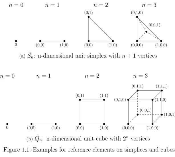
The individual elements t_i of the mesh typically have simple shape and in order to simplify the calculations t_i is given by a transformation from a reference element. In figure 1.1 shows different types of reference elements ˆt in different space dimensions that are used in practice: the simplex and the cube family.

Proposition 1.18 (Reference transformation). Every element t_i ⊂ Rⁿ, i ∈ T_h can be obtained from the reference element ˆt ⊂Rⁿ by using an invertible affine- linear transformation (shifting, rotation, scaling...)

µ_i : ˆS_n or Qˆ_n →t_i, t_i = µ_i(ˆt) =B_itˆ+z_i,

with B_i ∈ R^d×d, detB_i > 0 and z_i ∈ R^d.

As a consequence we have

Corollary 1.19. Ω is a polyhedral domain (polygon in two space dimensions)!

In general, nonlinear transformations µ can also be considered which then allows one to handle domains with curved boundaries but this will not be considered in this lecture.

It turns out that the meshT_hhas to satisfy the following additional properties:

1. Regularity of structure: Two cells have at most one vertex or one edge (or one face in 3D) in common (no “hanging nodes”).

(17)

0

n = 0

(0,0) (1,0)

n= 1

(0,0) (0,1)

(1,0)

n= 2

(0,0,0) (1,0,0) (0,0,1) (0,1,0)

n= 3

(a) Sˆn: n-dimensional unit simplex with n+ 1 vertices

0

n = 0

(0,0) (1,0)

n = 1

(0,0) (1,0) (0,1) (1,1)

n = 2

(0,0,0) (1,0,0) (0,0,1) (0,1,0)

(0,1,1)

(1,1,0) (1,1,1)

(1,0,1)

n = 3

(b) Qˆ_n: n-dimensional unit cube with 2ⁿ vertices

Figure 1.1: Examples for reference elements on simplices and cubes 2. Regularity of form: For every cell it holds

∃c₁ > 0 : h_t ≤c₁ρ_t

with the apothem ρ_t and the circumscribed radius h_t. 3. Regularity of size: Every cell is of the same size.

∃c₂ > 0 : max

t∈Th

h_t ≤ c₂min

t∈Th

h_t.

Remark 1.20. This only make sense if we have a sequence of grids T_h,ν and ν ∈ N such that h_ν → 0 and all constants c_i, i = {1,2}, are the same for every

ν.

Finite Element Spaces

Using the mesh we now we can construct Finite Element ansatz spaces and deal with questions about the practical realization of the method. Ω is a polygon domain with the decomposition T_h in triangles or rectangles (triangular pyramid or hexahedron in 3-D) and all the properties given above are satisfied.

(18)

Generally we define the following multivariate polynomial spaces of degree k or smaller:

Pⁿk := {u ∈ C^∞(Rⁿ) : u(x) = X

0≤|α|1≤k

c_αx^α},

Qⁿk := {u ∈ C^∞(Rⁿ) : u(x) = X

0≤|α|∞≤k

c_αx^α}

with |α|₁ = α₁ + ...+ α_n, |α|_∞ = max_i=1,...,nα_i and x^α = x^α₁¹ ·. . .·x^αⁿ. In R² this looks like

P²k := {u ∈ C^∞(R²) : u(x) = X

0≤i+j≤k

c_ijxⁱ₁x^j₂},

Q²k := {u ∈ C^∞(R²) : u(x) = X

0≤i,j≤k

cijxⁱ₁x^j₂} With that we may define the following function spaces:

P_kⁿ(T_h) := {u ∈ C⁰(Ω) : ∀t ∈ T_h : u

t ∈ Pⁿk}, Qⁿ_k(T_h) := {u ∈ C⁰(Ω) : ∀t ∈ T_h : u

t = ˆu_t ◦µ⁻¹_t ,uˆ_t ∈ Qⁿk}.

It can be checked that this definition is in fact proper, i.e. the requirement of global continuity does not contradict the polynomial form within each element.

The next step is to construct a basis for the finite element space. In particular, for the finite element spaces considered here, a so-called Lagrange basis can be found which is characterized by the property

ϕ^h_i(s_j) =δ_ij, j = 1, ..., N_h,

for certain points s_j. In the lowest order case k = 1 the pointss_j are the vertices of the mesh T_h.

Approximation Properties of FE spaces

Definition 1.21 (Lagrange-Interpolation). Given a Lagrange basis we can define the Lagrange interpolation operator acting on continuous functions:

I :C⁰(Ω) → P_kⁿ(T_h), Iv =

N_h

X

i=1

v(s_i)ϕ^h_i. Remark 1.22. Note that Iv_h ≡ v_h for every v_h ∈ P_kⁿ(T_h).

(19)

Remark 1.23. In order to define Lagrange interpolation for Sobolev functions we need k > ⁿ₂ for H^k(Ω) ⊂ C⁰(Ω). Then the Sobolev embedding theorem ensures that functions are continuous and pointwise evaluation is well-defined.

This means for n = 1 that k ≥ 1 and for n= 2,3 that k ≥ 2.

A cornerstone of the finite element a-priori error estimate is the following approximation property of finite element functions:

Proposition 1.24. For k ∈ N, k > min(1, n/2) and Lagrange interpolation I : H^k(Ω) → P_k−1ⁿ (T_h) (note the polynomial degree is k−1!) and m ∈ {0,1}

we have the estimate

ku− Iuk_m,Ω ≤ch^k−m|u|_k,Ω

with a constant c = c(n, k,ˆt,T_h). In particular, the constant depends on the

size of the angles of the triangulation.

As an example consider n = 2 and k > 1 (required to make Lagrange interpolation well-defined), i.e. the smallest k is 2 and the corresponding polynomial degree is 1 (piecewise linear functions). Then we have ku− Iuk_1,Ω ≤ ch|u|_2,Ω. However, the Lax-Milgram theorem establishes only a solution in H¹. Thus one has to assume that a solution with “additional regularity” exists.

Regularity Assumptions

We now discuss briefly under which assumptions solution in higher-order Sobelev spaces actually do exist.

Example 1.25. For domains with smooth boundary or convex polygonal domain Ω it has been proved that u ∈ H²(Ω).

Example 1.26. Ω has a C^s boundary ∂Ω (s times continuously differentiable parameterized), then one can show u ∈ H^s(Ω).

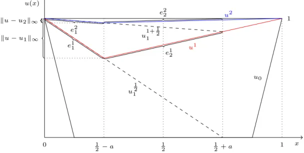
The regularity of solutions of problem (1.2) can be also “very low”. For this discussion fractional order Sobolev spaces are required, i.e. H^s(Ω) with s ∈ R. Example 1.27. Consider the problem−∇·(K(x)∇u) = f (in weak form) where the coefficient K(x) > 0 is discontinuous and has the following “checkerboard”

form:

K₁ K₂

K₂ K₁

(20)

Then one can show that for 0 < K₁ ≤ K₂ the solution satisfies u ∈ H^1+α with α = ²_πarctan

2√ K1K2

K2−K1

≈ ⁴_πq

K₁

K2 which approaches zero for K1 K2. Correspondingly, the convergence of the finite element method is h^α which is

extremely slow and is observed in practice.

A-priori Error Estimates

We start with a very important property of the finite element solution.

Proposition 1.28 (Galerkin orthogonality). Suppose u ∈ V solves (1.2) and uh solves (1.6), i.e.

a(u_h, v_h) =l(v_h) ∀v_h ∈ V_h. (1.7) Then it follows that the error e = u−u_h satisfies

a(e, v_h) = 0 v_h ∈ V_h.

Proof. Since V_h ⊂V, we can use v_h as the test function in the original equation a(u, vh) = l(vh) ∀v_h ∈ Vh.

Subtracting from this equation (1.7), we get the Galerkin orthogonality relation for the error u−u_h:

a(u−uh, vh) =a(u, vh)−a(uh, vh) = l(vh)−l(vh) = 0 ∀v_h ∈ Vh.

If a(·,·) defines a scalar product on V, which it does in the symmetric case, then we can conclude that the error is orthogonal (w.r.t. the scalar product a(·,·)) to all functions in Vh.

An important consequence of Galerkin orthogonality is

Lemma 1.29 (Céa’s lemma). The bilinear form a : V ×V → R, V = H₀¹(Ω), fulfills the properties

• continuity: |a(v, w)| ≤ Ckvk_1,Ωkwk_1,Ω for some constant C > 0 and all v, w ∈ V and

• coercivity: a(v, v) ≥ αkvk²_1,Ω for some constant α > 0 and all v ∈ V. Then the error satisfies

ku−u_hk_1,Ω ≤ C α inf

v_h∈V_hku−v_hk_1,Ω ∀v_h ∈ V_h.

The infimum term characterizes the best approximation of u in the subspace V_h

with respect to the H¹-norm.

Céa’s lemma together with the approximation property gives the a-priori estimate.

(21)

Theorem 1.30 (A priori error estimate). For the error u−u_h between the exact solution u ∈ V and the FE solution u_h with the ansatz space V_h ⊂ H₀¹(Ω) of order k ≥ 1, the polynomial degree of the ansatz functions, it holds the a priori error estimation

ku−uhk_1,Ω ≤ch^k−1|u|_k,Ω,

whereby the dimension n ≤ 3 and the solution is required to be in H^k(Ω).

In the L²-norm one can show

ku−uhk_0,Ω ≤ ch²|u|_2,Ω for polynomial degree 1.

Practical Implementation of the matrix A^h

In this section we want to present a systematic way to compute the entries of the stiffness matrix A^h ∈ R^N^h^×N^h for the elliptic problem

(K∇u,∇v) = (f, v) ∀v ∈ V.

This process is called “matrix assembly”. To assemble the linear system of equations,

A^hz^h = b^h,

we use a cell-wise computation of the necessary integrals. The definition of the matrix entry is

(A^h)ij = a(ϕ^h_j, ϕ^h_i) = Z

Ω

(K∇ϕ^h_j)· ∇ϕ^h_i dx.

Now we split the domain into elements to arrive at (A^h)_ij = X

t∈Th

Z

t

(K∇ϕ^h_j)· ∇ϕ^h_i dx.

We calculate the contribution of one element with the help of the reference transformation µ_t from 1.18. On element t we have the relation

ˆ

v(ˆx) = v(µ_t(ˆx)) (1.8)

between the finite element function v on the element t ∈ T_h and the corresponding function on the reference element. Recall that for affine transformations we

(22)

have µ_t(ˆx) = B_txˆ+z_t and B_t = ˆ∇µ_t(ˆx) (the hat on the gradient operator means differentiation with respect to x). The transformation formula for integralsˆ

Z

t

v(x)dx = Z

ˆt

ˆ

v(ˆx)|detB_t|dˆx

then establishes that we can calculate the required integral on the reference element.

In addition, from the chain rule applied to (1.8) it follows

∇v(µ_t(ˆx)) = B_t^−T∇ˆˆv(ˆx).

Using all these relations the matrix entry can be computed as (A^h)_ij = X

t∈Th

Z

tˆ

[K(µ_t(ˆx)) ˆ∇µ_t(ˆx)−T∇ˆϕˆ_j(ˆx)]· ∇µˆ _t(ˆx)−T∇ˆϕˆ_i(ˆx)|det ˆ∇µ_t(ˆx)|dˆx.

In practice the computations are organized such that all integrals on the element tcontributing to differenti, j are computed consecutively so that the (expensive) evaluations of µ_t (Jacobian and determinant) can be reused. Moreover, the evaluations of (gradients of) the basis functions ϕˆ^h_i on the reference element can be computed once and stored.

A posteriori error estimation

An important role in partial differential equations is error control. Of interest is to estimate the error between an approximate solution u_h and the exact solution u. For this purpose we have the “a posteriori error estimator”, which only depends on calculated quantities and the data f. The a priori error in the previous section is not useful to control the error, because the necessary information about higher-order derivatives of the exact solution u are not available.

Theorem 1.31. For the error u−u_h there holds the psteriori error estimate ku−u_hk_1,Ω ≤ c

X

t∈Th

h²_tkRk²_0,t+ X

γ∈F_hⁱ∪F_h^N

h_γkrk²_0,γ ¹₂

with the strong formulation of the elliptic operator R = f + ∇ ·(K∇u_h)

| {z }

= 0forP1-elements

−c u_h,

(23)

the jump terms over the edges γ ∈ F_hⁱ and the error in the Neumann boundary condition γ ∈ F_h^N

r(x) =

([−(K∇u_h)·ν] x∈ γ ∈ F_hⁱ

−(K∇u_h)·ν −j x∈ γ ∈ F_h^N .

The constant c depends on the mesh and the polynomial degree and is hardly

computable in practice.

Interpolation of non-smooth functions

The Lagrange interpolation requires enough regularity of the Sobolev function.

In certain situations, such as for the a-posteriori error estimate given above, on requires a finite element interpolation that can work directly on H¹ functions.

One possibility is the local “Clement” interpolation 1.32:

Definition 1.32 (Clement interpolation). For every function v ∈ H¹(Ω) exists the “Clement” interpolation C_hv ∈ V_h:

C_h : H¹(Ω)→ V_h ⊃ P₁ⁿ(T_h),

which is a combination of the Lagrange interpolation and the following L²-

projection.

Remark 1.33. The Clement interpolation is not a projection, i.e. C_hC_hv 6=

Chv.

Another option is the “L²-projection” 1.34, which is orthogonal but not local.

Definition 1.34 (L²-projection). TheL²-projectionQ_h : L²(Ω) →V_his defined by

(Q_hv, w_h)_0,Ω = (v, w_h)_0,Ω ∀w_h ∈ V_h with the estimate

kv −Q_hvk_0,Ω ≤ ch|v|_1,Ω.

(24)

(25)

Chapter 2 Classical Iterative Methods

2.1 Linear Iterative Methods

The regular linear system

Ax = b (2.1)

is solved by constructing a sequence x⁰, x¹, . . . with arbitrary initial guess x⁰ that converges towards the solution x. One way to construct linear iterative methods is via defect correction. For arbitrary x^k define the error as

e^k := x−x^k. (2.2)

Due to linearity we have

Ae^k = Ax−Ax^k = b−Ax^k := d^k (2.3) which is called defect. Note that d^k = b−Ax^k can be readily computed while the underlying error e^k is usually not available.

In order to arrive at an iterative method A on the left hand side of (2.3) is replaced by some approximation W, i.e. we solve W v^k = d^k and v^k = W⁻¹d^k approximates e^k. This gives us the generic form of a linear iterative method:

x^k+1 = x^k+ W⁻¹(b−Ax^k). (2.4) Particular choices for W are

W_Ric = ω⁻¹I ω ∈ R,Richardson W_{J ac} = diag(A) Jacobi

W_GS = L+D A = L+D + U,Gauß-Seidel

Analysis of linear iterative methods is based on the error propagation equation e^k+1 = x−x^k+1

= x−x^k −W⁻¹(Ax−Ax^k)

= (x−x^k)−W⁻¹A(x−x^k)

= e^k −W⁻¹Ae^k

= (I −W⁻¹A)e^k =: Se^k The matrix S = I −W⁻¹A is called iteration matrix.

(26)

Definition 2.1.

σ(A) := {λ ∈ C : λ is eigenvalue of A}

is called the spectrum of A and

ρ(A) := max{|λ| : λ ∈ σ(A)}

is called the spectral radius of A.

Theorem 2.2. A, W regular matrices. Then the iterative scheme (2.4) converges if and only if ρ(S) < 1.

Proof. See Hackbusch [1991]. Idea: e^k = S^ke⁰ and show S^k → 0. For diagonalizable matrices this is easy to see as S^k = T D^kT⁻¹ and D^k = diag(λ^k₁, . . . , λ^k_N) a diagonal matrix. The argument can be extended to non-diagonalizable matrices.

In general it is difficult to determine ρ(S). One option is to use a norm estimate

e^k+1 ≤ (I −W⁻¹A)e^k

⇒ ke^k+1k ≤ kI −W⁻¹Ak ke^kk

for any submultiplicative matrix norm. Since ρ(S) ≤ kSk for any norm and kSk < 1 is required for convergence, the norm needs to be chosen carefully.

A special case are symmetric positive definite matrices where the spectral radius can be computed exactly and related to the condition number.

Theorem 2.3. A, B symmetric and positive-definite matrices. Then the iteration

x^k+1 = x^k+ 1

λ_max(BA)B(b−Ax^k) converges with the rate

ρ = 1− 1 κ(BA) where

κ(BA) = λ_max(BA) λ_min(BA)

is the spectral condition number and λ_max(BA), λ_min(BA) are the extreme eigenvalues of BA.

(27)

2.1 Linear Iterative Methods

Proof. A is symmetric positive definite, so there is an unitary matrix Q such that A = QDQ^T with D = diag(λ₁, . . . , λ_N) with λ_i ∈ σ(A) ⊂ R⁺. Set D¹² := diag(√

λ₁, . . . ,√

λ_N) and A¹² := QD¹²Q^T. Then we have σ(BA) = σ(A¹²BAA⁻¹²) = σ(A¹²BA¹²). Since T := A¹²BA¹² is symmetric and positive definite all eigenvalues of BA are real and positive. Now T is also diagonalizable and has a complete set of eigenvectors. Since σ(S) = σ(I − _ω¹T) = {µ_i : µ_i = 1−^λ_ωⁱ for λ_i ∈ σ(T) =σ(BA)}, settingω = λ_max(T)we get µ_i ∈ [0,1−_λ^λ^min^(T⁾

max(T)].

So ρ(S) = 1− _κ(T¹ ₎.

For B = I we obtain the Richardson iteration W = _λ ¹

max(A)I. For B = A⁻¹ we have κ(BA) = 1 and ρ(S) = 0.

The matrixB is supposed to reduce the condition number ofAand is therefore often called a preconditioner.

Now what is the condition number of A?

Observation 2.4 (Raleigh Quotient). LetA ∈ R^n×n be symmetric and positive definite. Then the extreme eigenvalues can be characterized by

λmin(A) = inf

x6=0

hAx, xi

hx, xi , λmax(A) = sup

x6=0

hAx, xi hx, xi , where h., .i is any scalar product in Rⁿ.

Proof. 1. Let h., .i be the Euclidean scalar product. There exists Q with A = Q^TDQ and QQ^T = I. Then

hAx, xi

hx, xi = hDQx, Qxi hQx, Qxi =

PN

i=1λ_i(Qx)²_i hQx, Qxi . From λ_minhQx, Qxi ≤ PN

i=1λ_i(Qx)²_i ≤ λ_maxhQx, Qxi we conclude the result.

2. Extend to hu, vi_M = hM u, vi = hM¹²u, M¹²vi.

Lemma 2.5. Let A_h be obtained from a Finite Element discretization of the Poisson equation, i.e. (A_h)_ij = a(φ_j, φ_i), using Lagrange basis functions of P₁ on a mesh of size h. Then there exists a constant c such that

κ(A_h) ≤ ch⁻² and the estimate is sharp.

Proof. Let h., .i be the Euclidean scalar product. We write Ω_ij := supp(φ_i) ∩ supp(φ_j).

(28)

hA_hx, xi =

N_h

X

i=1 N_h

X

j=1

x_ix_ja(φ_j, φ_i)

=

N_h

X

i,j=1

x_ix_j Z

Ωij

∇φ_j · ∇φ_idx

=

N_h

X

i,j=1

x_ix_j X

t∈Ωij

Z

ˆt

(B_t^−T∇φˆ_j)·(B_t^−T∇φˆ_i)|detB_t|dˆx (*)

≤

Nh

X

i=1

xi





Nh

X

j=1

xj

X

t∈Ωij

ch^d−2





= ch^d−2hEx, xi

≤ch^d−2kExk kxk

≤ch^d−2kEk₂kxk²

= ch^d−2kEk₂hx, xi where

Eij :=

(1 Ω_ij = supp(φ_i)∩supp(φ_j) 6= ∅ 0 otherwise.

Note that kEk₂ ≤ K when E symmetric and kEk_∞ = K. In (*) we used the estimates

kB_t^−Tk ≤ c1

h, |detB_t| ≤ ch^d and k∇φˆ_ik ≤ 1.

Dividing by hx, xi and taking the supremum then shows

λ_max(A_h) = sup

x6=0

hA_hx, xi

hx, xi ≤ ch^d−2.

Now we give an estimate for λ_min and recognize that based on the Lagrange

(29)

2.2 Block Iterative Methods

basis functions we have for any function u_h = PN_h

i=1x_iφ_i: hA_hx, xi = a(u_h, u_h)

≥ αku_hk²_1,Ω

= α(ku_hk²_0,Ω+|u_h|²_1,Ω)

≥ α(ku_hk²_0,Ω+ 1

s²ku_hk²_0,Ω) (Friedrich inequality: assume ΓD 6= 0)

≥ α1 +s²

s² ku_hk²_0,Ω

≥ α1 +s²

s² h^dhx, xi (not shown here) and thus

λ_min(A_h) = inf

x6=0

hA_hx, xi

hx, xi ≥ α1 +s² s² h^d Together we obtain

κ(Ah) = λ_max(A_h)

λ_min(A_h) ≤ch⁻².

2.2 Block Iterative Methods

These are precursor to overlapping Schwarz methods.

The following notation is handy when displaying block methods and describing the parallel implementation of iterative methods.

Index sets

An index set I is a finite subset of N⁰. In particular index sets need not be consecutive or starting with 0 or 1. x∈ R^I is the vector having components(x)_i for all i ∈ I. Alternatively identify a vector x ∈ R^I with the map x : I →R.

Analogously, for any two index sets I, J ⊂ N⁰: A ∈ R^I×J is the matrix with entries (A)_i,j for all (i, j) ∈ I ×J. Alternatively: A: I ×J → R.

Subvectors and submatrices

Let I˜⊂I and J˜⊂J. Then, for x ∈ R^I, x_I_˜ is given by (x_I_˜)_i = (x)_i for all i ∈ I˜ and for A∈ R^I×J, AI,˜J˜ is given by (AI,˜J˜)_i,j = (A)_i,j for all (i, j) ∈ I˜×J˜.

Displaying a representation of a vector or matrix requires an ordering of the index sets, e.g. the lexicographic ordering. Also, certain iterative methods, e.g.

Gauß-Seidel, require an ordering of the index set.

(30)

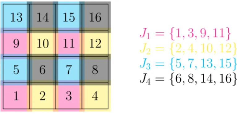
Partitioning

Block methods are based on a partitioning of the index set I ⊂ N⁰. Let P = {1, . . . , p} be the index set of the blocks and choose I_i ⊆ I for i ∈ P such that

[

i∈P

I_i = I and I_i ∩I_j = ∅ for all i 6= j.

Block-Jacobi and Block-Gauß-Seidel

Then the Block-Jacobi and Block-Gauß-Seidel methods are defined by (W_{BJ ac})_i,j =

((A)_i,j if i, j ∈ I_k for a k ∈ P

0 else,

(WBGS)i,j =

((A)_i,j if i ∈ I_k, j ∈ I_l for l ≤ k and k, l ∈ P

0 else .

Assume that the index set I is ordered such that i < j whenever block(i) < block(j) where block(i) =k :⇔i ∈ Ik. Then

W_{BJ ac} =







AI₁,I₁ 0 . . . 0 0 A_I₂_,I₂ ...

... . .. ... 0 . . . A_I_p_,I_p







, W_BGS =







AI₁,I₁ 0 . . . 0 A_I₂_,I₁ A_I₂_,I₂ ...

... . .. ... A_I_p_,I₁ . . . A_I_p_,I_p





 .

Both methods require the solution of the p smaller systems A_I_i_,I_i. Algorithmic Formulation

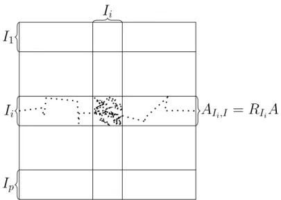
Define the rectangular restriction matrix

R_I_i :R^I → R^Iⁱ, (R_I_ix)_α := (x)_α∀α ∈ I_i.

RI_i is a |I_i| × |I| matrix with exactly one 1 per row. All 1s are in different columns, so rankR_I_i = |I_i|.

With this we can write

A_I_i_,I_i = R_I_iAR_I^T_i and get for the Block-Jacobi method

x^k+1 = x^k +X

i∈P

R^T_I

iA⁻¹_I

i,IiR_I_i(b−Ax^k)

(31)

2.3 Descent Methods

where the computations can be done in parallel. In case of the Block-Gauß-Seidel method we get

For i = 1, . . . , p : x^k+^pⁱ = x^k+ⁱ⁻¹^p +R^T_I_iA⁻¹_I

i,I_iR_I_i(b−Ax^k+ⁱ⁻¹^p ).

Without further assumptions on Ii andA these corrections have to be computed sequentially!

For the convergence of the block variants one can prove:

Theorem 2.6. A let be symmetric positive definite.

1. 2W_{BJ ac} −A be symmetric and positive definite then kS_{BJ ac}k_A < 1.

2. kS_BGSk_A < 1 where kSk_A is the matrix norm associated to the energy norm kxk_A := p

hAx, xi.

Proof. See [Hackbusch, 1991, Satz 4.5.4 and 4.5.6].

2.3 Descent Methods

These are nonlinear iterative methods based on minimizing the functional F(x) = 1

2hAx, xi − hb, xi.

Theorem 2.7. A symmetric and positive definite. Then the unique minimum x^∗ of F coincides with the solution of the linear system Ax= b.

Proof. For any x = x^∗ + v show F(x) = F(x^∗) + ¹₂hAv, vi > F(x^∗) if v 6= 0.

Uniqueness is proven by contradiction.

1D-minimization

Given an iterate x^k and a “search direction” p^k one can easily solve the problem Find α ∈ R such that F(x^k +αp^k) → min

by

α = (p^k)^T(b−Ax^k)

(p^k)^TAp^k . (2.5)

Gradient descent method: Choose p^k = −∇F(x^k) = b−Ax^k.

Theorem 2.8. A symmetric and positive definite. Then, with x being the solution of Ax = b, the gradient descent method satisfies

kx−x^kk_A ≤ κ(A)−1

κ(A) + 1kx−x^k−1k_A.

(32)

Algorithm 2.1 Gradient Descent Method

Given: Initial guess x, right-hand side b and tolerance < 1 d := b−Ax

δ := δ₀ := kdk while δ > δ₀ do

q := Ad . matrix vector product

α := hd, di/hd, qi . scalar products

x := x+αd . x update

d := d−αq . d = b−A(x+ v) =b−Ax−Av = d−Av

δ := kdk . recompute norm

end while

Proof. See [Hackbusch, 1991, Theorem 9.2.3].

The convergence factor can be written has κ(A)−1

κ(A) + 1 ≤ 1− 1 κ(A) + 1.

So for large κ(A) the convergence factor nearly the same as that of the damped Richardson method.

Preconditioning

Idea: Choose M regular and multiply Ax= bto the left with M⁻¹ to obtain the equivalent system M⁻¹Ax = M⁻¹b (left preconditioning). If κ(M⁻¹A) κ(A) then the convergence of the gradient method applied to this system is better.

However, in general, M⁻¹A is not symmetric even when M and A are symmetric. Assume M and A are symmetric and positive definite. Then M¹² is well defined and

σ(M⁻¹A) = σ(M¹²M⁻¹AM⁻¹²) = σ(M⁻¹²AM⁻¹²).