Using Gene Duplication and Gene Deletion in Evolution Strategies

U N I V E R S I T Y OF D O R T M U N D

REIHE COMPUTATIONAL INTELLIGENCE COLLABORATIVE RESEARCH CENTER 531

Design and Management of Complex Technical Processes and Systems by means of Computational Intelligence Methods

Using Gene Duplication and Gene Deletion in Evolution Strategies

Karlheinz Schmitt

No. CI-187/04

Technical Report ISSN 1433-3325 November 2004

Secretary of the SFB 531 · University of Dortmund · Dept. of Computer Science/XI 44221 Dortmund · Germany

This work is a product of the Collaborative Research Center 531, “Computational

Intelligence,” at the University of Dortmund and was printed with financial support of

the Deutsche Forschungsgemeinschaft.

Using Gene Duplication and Gene Deletion in Evolution Strategies

Karlheinz Schmitt Universtit¨at Dortmund D-44221 Dortmund, Germany

Karlheinz.Schmitt@udo.edu Abstract- Self-adaptation is a powerfull mechanism in

evolution strategies (ES), but it can fail. The reasons for the risk of failure are manyfold. As a consequence pre- mature convergence or ending up in a local optimum in multimodal fitness landscapes can occur. In this article a new approach controlling the process of adapation is proposed. This approach combines the old ideas of gene deletion and gene duplication with the self-adaptation mechanism of the ES. In order to demonstrate the prac- ticability of the new approach several multimodal test functions are used. Methods from statistical design of experiments and regression tree methods are used to im- prove the performance of a specific heuristic-problem combination.

1 Introduction

In modern synthesis of evolutionary theory, gene duplica- tion emerged as a major force. In particular, redundant gene loci created by gene duplication are permitted to accumu- late formerly forbidden mutations and emerge then as ad- ditional gene loci with new functions. It is hardly surpris- ing that these major effect is not unconsidered in the de- sign of evolutionary algorithms. The first evolution strat- egy (ES) using operators like gene duplication and gene deletion can be found in Schwefel [Sch68]. Here the op- timization of a nozzle for a two-phase flow leads to surpris- ing good results. A good overview of existing approaches dealing with variable-length representations can be found in [Sch97, Bur98]. Unfortunately, most of the approaches are extremely application-oriented. Perhaps the most im- portant reason for the application oriented design is the re- strictive fixed-length, fixed-position representation of the solutions that are used in many search heuristics. Based on this fixed representation, the introduction of duplication and deletion leads to several problems. For instance, the role of positions in a fixed-length solution is destroyed. In order to design genetic operators which are able to generate interpretable solutions, the assignment problem of finding the locus of corresponding genes has to be solved. In most cases those solutions lead to extremely application oriented solutions [Har92, GKD89].

The main focus of this article lies on a more applica- tion independent approach. Starting from the idea of in- troducing gene duplication and gene deletion into ES, addi- tional genetic operators varying the number of used endoge- nous strategy parameters are introduced to generate a satis-

factory self-adaptation in various fitness landscapes. Ex- periences gained in the last four decades show that self- adaptation is a powerfull mechanism, but it can fail. The reasons for the risk of failure are manyfold. As a conse- quence premature convergence or ending up in a local opti- mum in multimodal fitness landscapes can occur. There- fore, various countermeasures should be found in litera- ture [Rec94, Her92, Tri97], but the main countermeasure in nature is gene duplication.

The rest of this article is organized as follows: in Sec- tion 2, an overview of the basic principles of the proposed search heuristic is given, followed by a brief description of the implementation details. In Section 3, a stastistical methodology to set up the experiments in an efficient man- ner is discussed. Experimental results are presented and dis- cussed in Section 4. Finally, Section 5 concludes this article with a summary of the insigths and with directions for fur- ther research.

2 Evolution Strategy

This section presents the main aspects of a multimembered evolution strategy (ES), since this was needed for further discussion. For a comprehensive introduction the reader is referred to [BS02, Sch95].

In principle, existing parameters in evolution strategies can be distinguished between exogenous and endogenous parameters. Exogenous parameters like µ (parent popu- lation size) or λ (member of descendants) which are kept constant during the optimization run, are a characteristic of most of the modern search heuristics. Endogenous param- eters are a pecularity of ES: they are used to control the ability of self-adaptation in ES during the run.

The adaptation of the endogenous parameters - the so called strategy parameters - depends on various adjust- ments. First of all, the strategy parameters are closely cou- pled with the object parameters [BS02]. Each individual has its own set of strategy parameters. Like the object param- eters, the strategy parameters undergo recombination (to- gether with the object parameters) and mutation and are used to control the mutation of the object parameters. Due to this mechanism, the optimizer can hope - and only hope - that an individual is able to learn the approximately optimal strategy parameters for the specific problem.

The realization of described self-adaptation mechanism

above depends further on the kind and the number of strat-

egy parameters to be adapted. In most cases only 1 or N

standard deviations are used. In the sphere function, i.e.

only one standard deviation [Sch95] will do the work ef- ficiently, in multimodal fitness landscapes it is favourable to use more than one standard deviation. The question of, how many standard deviations are necessary for a specific algorithm-problem combination or how many are necessary during of evolution, is still open.

Correlated mutations finalize the current self-adaptation mechanism in ES. For a deeper insight of correlated mu- tations the reader is referred to [Rud92]. The use of cor- related mutation introduces N(N − 1)/2 additional strat- egy parameters which have to be controlled, too. This may be the reason why correlated mutations are commonly not used. But in many real-world applications where the computational cost of optimization problems is determined mainly by the time-comsuming function evaluations, the computational effort for the optimization task will be rel- ativize.

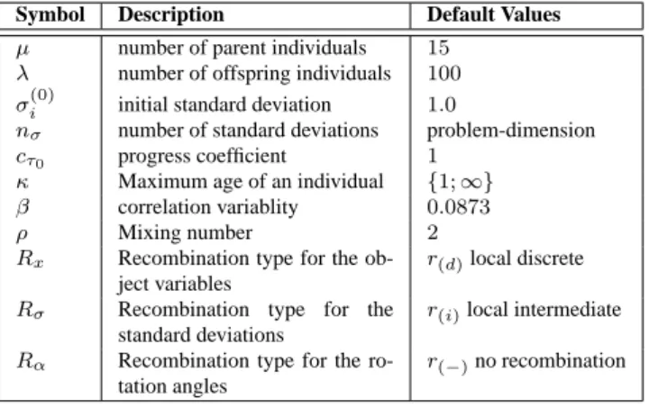
In order to obtain the best possible self-adaptation for the given problem the specification of the exogenous pa- rameters is required. Table 1 shows the main exogenous parameters used in ES and their common default parame- terizations.

Table 1: Exogenous parameters of an ES. Column 1 shows the usual symbols or the parameters. Column 3 holds com- momly used values [B¨ac96, Kur99].

Symbol Description Default Values µ number of parent individuals 15

λ number of offspring individuals 100 σ

initial standard deviation 1.0

n

number of standard deviations problem-dimension

c

progress coefficient 1

κ Maximum age of an individual {1; ∞}

β correlation variablity 0.0873

ρ Mixing number 2

R

Recombination type for the ob- ject variables

r

local discrete R

Recombination type for the

standard deviations

r

local intermediate R

Recombination type for the ro-

tation angles

r

no recombination

Some of these values originate from investigations in the sixties [Sch68, Rec71] of the last century about only two artificial test functions (sphere and corridor). Other values - such as the progress coefficient c

- are theoretically very well analyzed [Bey95], but also only for a specific test func- tion. Experimental investigations from [Kur99, B¨ac96] have yielded to principle recommendations for the parameter set- tings i.e. for the type of recombination that must be choosen if the test function is unimodal or multimodal or for the ini- tial standard deviation. But all of them state out that the use of these default values without reflection could be a mistake.

Nevertheless, after a first specification of these param-

eters, an evolution strategy is performed as follows: The initial parental population of size µ will be generated. A new offspring population is produced then by the rule of the (µ/ρ κ λ) - notation. From the parent population of size µ, ρ individuals are randomly choosen as parents for one child.

Depending on the specified types of recombination, the re- combination of the endogeneous and exogeneous parame- ters takes place. With respect to the recombination step, the mutation of the strategy parameters is done. The learning parameter τ determines the rate and precision of the self- adaptation of the standard deviations and β determines the adaptation of the rotation angles. After having a new off- spring population of size λ, the selection operator is used to select the new parental population for the next iteration.

κ = 1 referres to the well-known comma-selection scheme of an ES, and κ = +∞ to the plus-selection scheme.

2.1 Implementation details

As mentioned above, the implementation of the self- adaptation mechanism depends on the kind and the number of strategy parameters. Given an individual ~a = (~ x, ~ σ, ~ α), where ~ x is the vector of objective variables, ~ σ holds the set of standard deviations and ~ α the rotation angles. Each ES individual may include one up to N(N + 1)/2 endogenous strategy parameters. For the case 1 < n

< N the stan- dard deviations σ

, . . . , σ

are coupled with the corre- sponding object variables and σ

is used for the remaining ones. The number of rotation angles n

depends directly on n

[Sch95] or is explicit set to 0.

The new deletion and duplication operator work on the set of standard deviations (n

) only. The additional varia- tion operators are defined as follows:

Duplication Operator: With a predefined duplication probalitity (dup = 0.028) a duplication may occur if n

< N . The duplicated standard deviation is added then at the end of ~ σ. The rate of gene duplica- tion is taken from an investigation of [ML00]. Within their work an estimation of gene duplication rates of Drosophila, and C. elegans is given. This is a sur- prisingly high mutation rate compared to previous es- timations that recommended a mutation rate of 0.1%

per gene.

Deletion Operator: Vice versa a predefined deletion prob-

ability (del = 0.028) is used in order to delete the last

standard deviation in n

if n

> 1 or not. The dele-

tion of the last standard deviation is used because of

their direct coupling with the rotation angles.

3 Experimental Environment

3.1 Test Functions

Just as for any other search heuristic, evolution strate- gies need to be assessed concerning their effectiveness for optimization purposes. To facilitate a reasonably fair comparison of search heuristics a number of artificial test functions are typically used. Well-known test suites of single-criteria parameter optimization problems are those of De Jong [DeJ75], Schwefel [Sch95] and Flaudas et el. [FPA

99]. These test suites serve well as an archive.

In most cases only a selection was made taking into account that it is important to cover various topological character- istics of landscapes in order to test the heuristics concern- ing efficiency and effectiveness. In principle, Whitley et al. [WMRD95] and B¨ack and Michalewicz [BM97] propose five basic properties as selection criterias for a fair test suite.

The suite should contain unimodal functions in order to test the efficiency, they have to include high-dimensinal, mul- timodal functions and also constrained problems to simu- late typical real-world applications. Due to the possibility of the presence of noise in industrial applications test func- tions with randomly pertubed objective values have to be included to.

The following test suite is composed disregarding the presence of noise and constraints in real-world applications.

Sphere function (F

) [DeJ75]: This is an unimodal test function with a minimum at x ~

= ~ 0, with f ( x ~

) = 0.

For a test of efficiency, this is the most used fitness function.

f (~ x) = P

i=1

x

. (1)

where

Start Point: x

= 10 ∀i ∈ {1, . . . , n}.

Double Sum (F

) [Sch95]:

f (~ x) = P

( P

j=1

x

)

. (2) where

Start Point: x

= 10 ∀i ∈ {1, . . . , n}.

Generalized Rastrigin function (F

) [TZ89]: This is a multimodal function. The constants are give by A = 10 and ω = 2π. Here the global optima is at x ~

= ~ 0, with f( x ~

) = 0.

f (~ x) = n · A + P

i=1

x

− A cos(ωx

). (3) where

Start Point: x

= 4 ∀i ∈ {1, . . . , n}.

Generalized Ackley function (F

) [BRS93]: This gen- eral extension of an originally two-dimensional test function is multimodal. Their constants are given by a = 20, b = 0.2 and c = 2π.

f (~ x) = −a exp[−b(

P

i=1

x

)

]−

exp[

P

i=1

cos(cx

)]+

a + exp(1) · exp(1).

(4)

where

Start Point: x

= 25 ∀i ∈ {1, . . . , n}.

Fletcher and Powell (F

) [RF63]: The constants a

, b

= [−100, 100] and α

∈ [−π, π] are randomly choosen and specify the position of the local minima.

The minimum is f (α) = 0. The matrices A and B are taken from B¨ack [B¨ac96].

f (~ x) = P

i=1

(A

− B

)

(5) where

A

= P

j=1

(a

sin α

+ b

cos α

) B

= P

j=1

(a

sin x

+ b

cos x

) Start Point: x

= 2.51818 ∀i ∈ {1, . . . , n}.

3.2 Choice of Parameter Settings

As mentioned in Section 2 many of so called default pa- rameterizations are proposed for the multimembered ES. In Table 1 usual default values are listed. But again, each heuristic-problem combination requires its specific parame- terization. Therefore, as long as the success or failure of a heuristic depends on (nearly) optimal parameter settings, it is neccessary to look for the optimal set of parameters anew.

Manyfold methods are proposed to tackle this problem.

A good overview can be found in [Kle87, BB03]. In this study, tree based methods, fractional factorial designs as well as classical regression analysis are used [BFOS84, Kle87, BBM04] in order to achive good parameter settings and to analyze the obtained results.

Fractional factorial designs are constructed by choosing

a certain subset of all the possible 2

combinations from a

full factorial design. The advantage of reducing the com-

putational effort is in opposite to the disadvantage of con-

founding. From now on it is possible that for several dif-

ferent effects the same algebraic expression is used, so it is

impossible to differentiate between these two effects, these

effects are called confounded. A good way to handle this

problem is the concept of resolution. A 2

fractional fac-

torial design is of resolution R if no q-factor effect is con-

founded with another effect that has less than R − q fac-

tors [GB78]. For a first screening phase, where only the

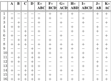
Table 2: Fractional factorial design 2

. This design rep- resents the starting design which is used for all test func- tions using correlated mutations with duplication and dele- tion probability > 0. If no correlated mutations, or duplica- tion/deletion oparetors are used, the values were set to 0.

A B C D E=

ABC F=

BCD G=

ACD H=

ABD I=

ABCD J=

AB K=

AC

1 − − − − − + + + − + +

2 + − − − + + − − + − −

3 − + − − + − + − + − +

4 + + − − − − − + − + −

5 − − + − + − − + + + −

6 + − + − − − + − − − +

7 − + + − − + − − − − −

8 + + + − + + + + + + +

9 − − − + − + + + − + +

10 + − − + + + − − + − −

11 − + − + + − + + + − +

12 + + − + − − − − − + −

13 − − + + + − − − + + −

14 + − + + − − + + − − +

15 − + + + − + − − − − −

16 + + + + + + + + + + +

main effects but no interactions are of interest, a resolution three design is sufficient. It ensures only that no main effect is confounded with each other main effect. Table 2 shows a 2

design, where the minus and the plus signs denote to the low and the high levels of the factors. The resulting de- sign matrix for the high and the low levels of the evolution strategy is shown in Table 3.

3.3 Methods of Analysis

Classical methods of statistical analysis such as regression analysis can be extend by tree-based regression methods.

A detailed example can be found in [BB03]. Here, it is shown that using regression trees the practitioner is able to screen out important parameter settings. One of their main advantages, besides their simplicity of interpretation, is that they do not require any assumptions about the underlying distribution of the responses.

The construction of a regression tree is a kind of variable selection similar to stepwise selection from classical ones, and rely on three components [BFOS84]:

• a set of questions upon which to base a split,

• splitting rules and goodness-of-split criteria for judg- ing how good a split is and

• the generation of summary statistics for terminal nodes.

In principle, a set of questions of the form

Is X ≤ d ? (6)

Table 3: Corresponding 2

fractional factorial design for the choosen ES parameterization.

µ λ N σ κ ρ dup del σ

R

R

R

10 60 1 1 2 0.001 0.001 0.15 d d d 20 60 1 1 20 0.001 0.028 3.0 i i i 10 120 1 1 10 0.028 0.001 3.0 i i d 20 120 1 1 2 0.028 0.028 0.15 d d i 10 60 5 1 10 0.028 0.028 0.15 i d i 20 60 5 1 2 0.028 0.001 3.0 d i d 10 120 5 1 2 0.001 0.028 3.0 d i i 20 120 5 1 20 0.001 0.001 0.15 i d d 10 60 1 +∞ 2 0.028 0.028 3.0 i d d 20 60 1 +∞ 20 0.028 0.001 0.15 d i i 10 120 1 +∞ 10 0.001 0.028 0.15 d i d 20 120 1 +∞ 2 0.001 0.001 3.0 i d i 10 60 5 +∞ 10 0.001 0.028 3.0 d d i 20 60 5 +∞ 2 0.001 0.028 0.15 i i d 10 120 5 +∞ 2 0.028 0.001 0.15 i i i 20 120 5 +∞ 20 0.028 0.028 3.0 d d d

is given, where X is a variable and d is a constant. The re- sponse to such a question is binary (yes/no). Each response partitions the tree into a left and a right node. This recur- sive procedure will continue, if one node contains enough experimental observations for another split.

4 Experimental Results

The following experiments were performed to investigate the question if the new duplication and deletion operator improve the performance of an evolution strategy when op- timizing multimodal fitness functions.

Therefore it is a common practice to compare the per- formance of the new algorithm including the additional op- erators with the standard implementation of the original al- gorithm. In order to ensure a relative fair comparison, both algorithms have to be tuned on the given heuristic-problem combination at first. This tuning step should be done with regression tree methods. In the following a detailed discus- sion on the 20-dimensional ackley function (F

) was per- formed. The other test functions were analyzed in a similar manner.

4.1 A Simple Tuning Step

First experiments, based on the experimental design shown in Table 3, were performed for both types of algorithms.

Due to simplification the experiments are devided into two main groups:

• Experiments without correlated mutations, and

• with correlated mutations.

For the first group the β, and the R

values from Table 3

are set to 0. Each of the 16 parameter settings was repeated

|

N=3,4,5,6,7,8,9,10,11,16,18,19,20

J=3

N=1,2

J=0.15 6.89 n=160

0.7813 n=108

0.0002294

n=70 2.22

n=38

19.58 n=52

Figure 1: Pruned regression tree for the modified ES opti- mizing a 20-dimensional Ackley function. The first split partitions the 160 experiments in the root node in two groups of 108 and 52 events. The average fitness value in the left node reads 0.7831 and in the right node 19.58. The first split is performed by the number of used standard devi- ations (N ).

Table 4: Corresponding ANOVA analysis. All observed fac- tors have a significant contribution to the results.

Df Sum

Sq

Mean Sq

F value

Pr(>F) J 1 3189.1 3189.1 455.752 < 2.2e − 16 K 1 229.4 229.4 32.783 5.843e − 08 N 14 9170.3 655.0 93.609 < 2.2e − 16 Residuals 143 1000.6 7.0

ten times, so that 160 observations are available for each algorithm in the group.

Figure 1 shows the pruned tree of the fitness values of function F

with correlated mutations using the ES with du- plication and deletion operators.

The first split partitions the N = 160 observations into groups of 108 (left node) and 52 (right node) observations.

The left group contains experimental runs with a great num- ber of standard deviations N = {3, . . . , 20} and an average fitness value of 0.7831, and the right node contains all ex- perimental runs, where the number of used standard devi- ations remains very small N = {1, 2} with an average fit- ness value of 19.58. Following the tree down to the node with the smallest average fitness value 2.294E − 4 the re- gression tree indicates that the initial value of the standard deviation (J) is significant for the success of the evolution runs. The corresponding classical analysis (Table 4) indi-

|

I=20

J=3

A=20

I=1

J=0.15

A=10

17.74 n=158

15.55 n=78

15.21 n=38

14.56

n=19 15.86

n=19

15.88 n=40

19.86 n=80

Figure 2: Pruned regression tree for the standard ES opti- mizing a 20-dimensional Ackley function. The first split partitions the 158 experiments in the root node into two groups of 78 and 80 events. The average fitness value in the left node reads 15.55 and in the right node 19.86. The first split is performed by the number of used standard devi- ations (I).

cates that the initial state (J ), the number of used standard deviations (N ), and the duplication (K) probability are sig- nificant for the obtained results.

The first 160 results indicate that a high value for the ini- tial standard deviation improves the performance. But this is not an unexpected result keeping in mind that the initial- ization of the first population of every algorithm takes place by choosing a single start point. As a consequent the ini- tial population remains in a relativ small area of the fitness landscape. The extension of this area is defined by the ini- tial standard deviation. The greater the value the greater the covered area. In multimodal fitness landscapes, this type of initialization is not a disdained factor. It may also be the rea- son, why in many ES the traditional initialization is changed to the initialization that is usually in genetic algorithms.

A relative high number of standard deviations (J ) used during the evaluation runs seems to be the most significant effect for the obtained results. Now, it could be conjectured that using the greatest possible number of standard devia- tions in the experiments (N

= N ) is the best choice for this parameter and therefore no additional variation opera- tors are neccessary. Figure 2 shows the pruned regression tree for the standard ES.

Although the amount of the used standard deviations is even significant as in the former case, the heuristic is not able to reach the global attractor area (fitness = 15.21).

Only in the initial phase of the optimization run, the self-

adaptation process with a great number of standard devia-

tions (left node) is able to steer the population through the

multimodal fitness landscape. But a high number of stan-

dard deviations does not seem to be the reason in itself for

Table 5: Parameter setting for the discussed heuristic- problem combination without correlated mutations.

Parameter modified ES

µ 20 20

λ 120 60

κ +∞ 1

R

intermediate discrete

R

discrete intermediate

R

none none

ρ 2 2

β 0 0

N

2 20

σ

3.0 3.0

dup 0.001 0.0

del 0.001 0.0

the good results from Fig. 1. This will be discussed in detail in the next section.

To begin with a fair comparison of both heuristics, re- gression tree methods as well as classical statistical methods are able to produce first statistically proved hints for nearly optimal parameter settings. For the given heuristic-problem combination the setting read:

4.2 Comparisons

A comparison of the standard ES and the modified ES with gene deletion and duplication operators was performed in this section. Again, each heuristic-problem combination was going through the discussed simple tunig step before the comparison was performed.

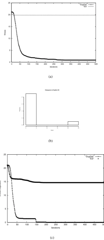
Figure 3 shows that – on a 20-dimensional Ackley func- tion - the ES working with duplication and deletion op- erators (DupDel) outperforms the standard ES (ES) in a significant manner. In Fig. 3(a) the arithmetic mean of ten independent runs without correlated mutations is de- picted, respectively. From these ten independent experi- ments nine runs of (DupDel) are able to reach the global attractor area 3(b). Only one run shows similar results as in the standard ES. In this single run the self-adaptation fails just as in all runs of the standard ES (ES). In the later case, the ES is not able to guide the population through the mulimodal fitness landscape. All populations end up in a local optimum.

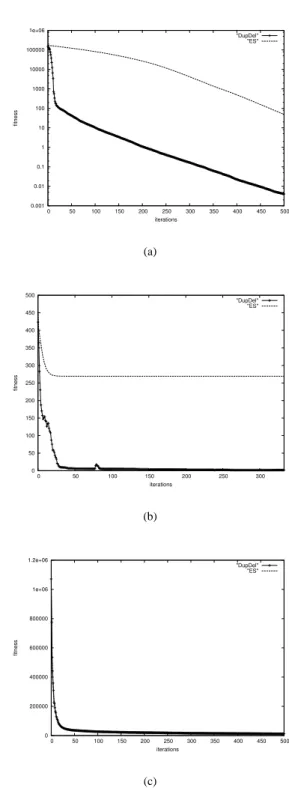
Quite different results can be observed, when using cor- related mutations (see Figure 3(c)). The single freak value in the former experiments from the DupDel model can be completely avoided, when using correlated mutations. In addition, a better convergence rate can be observed (150 iterations in contrast to 300). In Figure 4 results for test functions F

, F

, and F

are presented. In functions F

and F

similar results as in the Ackley function can be shown.

In function F

the convergence rate is on multiple regions superior to the standard ES. In case of function F

the mod-

0 5 10 15 20 25

0 50 100 150 200 250 300 350 400 450 500

fitness

iterations

"DupDel"

"ES"

(a)

Histogramm of DupDel−ES

fitness

Frequency

0 5 10 15 20 25

02468

(b)

0 5 10 15 20 25

0 50 100 150 200 250 300 350 400 450 500

fitness (logscale)

iterations

"DupDel"

"ES"

(c)

Figure 3: Figure (a) shows the arithmetic mean of ten inde-

pendent runs optimizing a 20-dimensional Ackley function

with using correlated mutations. Figure (b) shows the corre-

sponding histogramm plot. Figure (c) shows the arithmetic

mean of ten independent runs optimizing a 20-dimensional

Ackley function with correlated mutations.

Table 6: Comparison of both models optimizing the 20- dimensional sphere function. The number of performed ex- periments is set to 10.

Model median mean

fitness

variance F

ES

7.357e−77 1.022e−76 4.72442e − 153 F

DupDel

3.110e−77 2.913e−77 3.753419e−155 F

ES

6.227e−77 6.287e−77 9.179366e−155 F

DupDel

2.895e−77 3.009e−77 3.664180e−155

ified model is also able to achive the global attractor area in contrast to the other model. An exception could be found in function F

. Here, no improvement can be observed.

4.3 Discussion

In the last section it was shown that it could be favourable to use additional variation operators mimicing gene dele- tion and gene duplication from nature in order to solve multimodal problems - but why? Looking at the duplica- tion operator, a duplication take place with a probabilty of dup = 0.028 or 0.001. In case of N

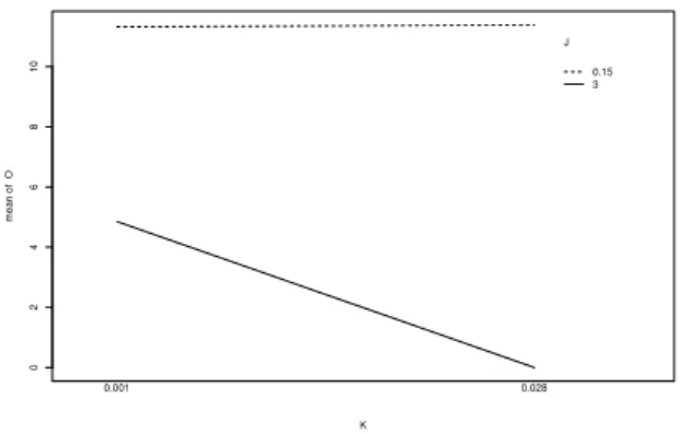
= 1 before dupli- cation, the single strategy variable is – depending on the number of iterations – more or less adapted to the local fit- ness landscape. Now, adding a second strategy variable the first endogenous variable controls the first objective variable only, the second controls all the rest. In the early stage of the optimization this will lead to relative great jumps in the fitness landscape. The more duplication and the greater the initial standard deviations the greater the fluctuations in the fitness values. In multimodal landscapes this effect could be high enough to guide a hole population out of a local optimum. In Figure 5 an interaction plot between the du- plication probability (K = {0.028, 0.001}) and the sizes of the inital standard deviation (J = {0.15, 3}) is shown. The greater the duplication probability and the greater the initial standard deviation the lower (better) the mean of the fitness (O). Therefore, the conjecture could be confirmed.

On the other side it must be also considered that this effect, which is favourable in the early stage of the evolu- tion run, is counterproductive for the end, when the global attractor area is achieved. In many test functions – here for example F

, and F

– when the global attractor area is achievd, the special case of a sphere function can be found. Therefore, both heuristics were set up on a 20- dimensional sphere function F

. Table 6 shows the obtained results. An extremely high number of fitness evaluations (F it

= 200000) was used in order to show the adapta- tion.

Despite of duplication and deletion, the modified ES is able to adapt the global optima in the same accuracy as the standard ES. The reasons could be found in the progress of the optimization run itself. During the run, the self-

0.001 0.01 0.1 1 10 100 1000 10000 100000 1e+06

0 50 100 150 200 250 300 350 400 450 500

fitness

iterations

"DupDel"

"ES"

(a)

0 50 100 150 200 250 300 350 400 450 500

0 50 100 150 200 250 300

fitness

iterations

"DupDel"

"ES"

(b)

0 200000 400000 600000 800000 1e+06 1.2e+06

0 50 100 150 200 250 300 350 400 450 500

fitness

iterations

"DupDel"

"ES"

(c)

Figure 4: Figure (a) shows the arithmetic mean of ten

independent runs optimizing a 20-dimensional Achwefel-

1.2 (F

) function without correlated mutations. Figure (b)

shows the obtained results for the generalized Rastrigin

function (F

) with correlated mutations, and finally Figure

(c) shows the results of function F

.

0246810

K

mean of O

0.001 0.028

J 0.15 3

Figure 5: Plot of the means of the fitness values. The la- bel on the x-axis represent different duplication probabili- ties (K = {0.0028, 0.001})

.

adaptation process leads to smaller and smaller standard de- viations, so if a duplication or deletion occurs, the noise will become smaller and smaller. Differences between both models seem to have vanished at the end of the evolution run.

5 Summary and Outlook

In this article additional variation operators mimicing gene duplication and gene deletion from nature were developed in order to improve the self-adaptation mechanism of evo- lution strategies. Self-adaptation is a powerful mechanism.

But even in multimodal fitness landscapes it can fail. On four multimodal test functions it was shown that using the new operators the risk of failure of the self-adaptation mech- anism can be reduced in a significant manner. This work will be extendend in the following way: To avoid the neces- sity of correlated mutations, the interaction between gene deletion and gene duplication operators has to be analyzed in detail.

Acknowledgments. Karlheinz Schmitt’s research was supported by the DFG as a part of the collaborative re- search center ‘Computational Intelligence’ (SFB 531) in Dortmund.

Bibliography

[B¨ac96] T. B¨ack. Evolutionary Algorithms in Theory and Practice. Oxford University Press, New York, 1996.

[BB03] T. Bartz-Beielstein. Experimental analysis of evolution strategies – overview and com-

prehensive introduction. Interner Bericht des Sonderforschungsbereichs 531 Compu- tational Intelligence CI–157/03, Universit¨at Dortmund, November 2003.

[BBM04] T. Bartz-Beielstein and S. Markon. Tuning search algorithms for real-world applications:

A regression tree based approach. Interner Bericht des Sonderforschungsbereichs 531 Computational Intelligence CI–172/04, Uni- versit¨at Dortmund, M¨arz 2004. (im Druck).

[Bey95] H.-G. Beyer. Toward a Theory of Evolu- tion Strategies: On the Benefit of Sex – the (µ/µ, λ)-Theory. Evolutionary Computation, 3(1):81–111, 1995.

[BFOS84] L. Breimann, J. Friedman, R. Ohlsen, and C.J.

Stone. Classification and Regression Trees.

Chapman and Hall, New York, 1984.

[BM97] T. B¨ack and Z. Michalewicz. Test landscapes.

In Handbook of Evolutionary Computation, pages B2.7:14 – B2.7.20. Oxford University Press, 1997.

[BRS93] T. B¨ack, G. Rudolph, and H.-P. Schwe- fel. Evolutionary programming and evolu- tion strategies: similarities and differences. In D. B. Fogel and W. Atmar, editors, Proc. Sec- ond Annual Conf. Evolutionary Programming (EP’93), pages 11–22, San Diego CA, 1993.

Evolutionary Programming Society.

[BS02] H.-G. Beyer and H.-P. Schwefel. Evolution strategies – A comprehensive introduction.

Natural Computing, 1(1):3–52, 2002.

[Bur98] D. S. Burke. Putting more genetics into ge- netic algorithms. Evolutionary Computation, 6(4):387–410, Winter 1998.

[DeJ75] K.A. DeJong. An Analysis of the Behavior of a Class of Genetic Adaptive Systems. PhD the- sis, University of Michigan, 1975.

[FPA

99] C.A. Flaudas, P.M. Pardalos, C.S. Adjiman, W.R. Esposito, Z.H. G¨um¨us, S.T. Hard- ing, J.L. Klepeis, C.A. Meyer, and C. A.

Schweiger. Handbook of Test Problems in Lo- cal and Global Optimization. Kluwer Aca- demic Publishers, 1999.

[GB78] J.S. Hunter G.E.P. Box, W.G. Hunter. Statis-

tics for experimenters. Wiley series in prob-

ability and mathematical statistics: Applied

probability and statistics. Wiley, 1978.

[GKD89] D. E. Goldberg, B. Korb, and K. Deb. Messy genetic algorithms: Motivation, analysis, and first results. Complex Systems, 3(5):493–530, October 1989.

[Har92] I. Harvey. The saga cross: The mechanics of recombination for species with variable- length genotypes. In R. M¨anner & B. Man- derick, editor, Parallel Problem Solving from Nature, volume 2, pages 269–281, 1992.

[Her92] M. Herdy. Reproductive isolation as strat- egy parameter in hierarchically organized evo- lution strategies. In Parallel Problem Solv- ing from Nature, pages 207–217, Amsterdam, 1992. Elsevier.

[Kle87] J.P.C. Kleijnen. Statistical Tools for Simula- tion Practioners. Marcel Dekker, New York, 1987.

[Kur99] F. Kursawe. Grundlegende empirische Un- tersuchungen der Parameter von Evolution- sstrategien - Metastrategien. PhD thesis, Uni- versity of Dortmund, 1999.

[ML00] J.S. Conery M. Lynch. The evolutionary fate and consequences of duplicate genes. Science, (290):1151–1155, 2000.

[Rec71] I. Rechenberg. Evolutionsstrategie: Optimie- rung technischer Systeme nach Prinzipien der biologischen Evolution. Dissertation, Tech- nical University of Berlin, Berlin, Germany, 1971.

[Rec94] I. Rechenberg. Evolutionsstrategie ’94, vol- ume 1 of Werkstatt Bionik und Evolutionstech- nik. Frommann–Holzboog, Stuttgart, 1994.

[RF63] M.J.D. Powell R. Fletcher. A rapidly conver- gent descent method for minimization. Com- put. J., 6:163–168, 1963.

[Rud92] G. Rudolph. On correlated mutations in evolution strategies. In R. M¨anner and B. Manderick, editors, Parallel Problem Solv- ing from Nature – Proc. Second Conf. PPSN, pages 105–114, Free University of Brussels, September 28–30, 1992. Elsevier, Amster- dam.

[Sch68] H. P. Schwefel. Experimentelle Optimierung einer Zweiphasend¨use, Teil I. Bericht Nr. 35 zum Projekt MHD–Staustrahlrohr 11.034/68, AEG Forschungsinstitut, Berlin, Oktober 1968.

[Sch95] H. P. Schwefel. Evolution and Optimum Seek- ing. Sixth-Generation Computer Technology.

Wiley Interscience, New York, 1995.

[Sch97] M. Sch¨utz. Other operators: Gene duplication and deletion. In Th. B¨ack, D. B. Fogel, and Z. Michalewicz, editors, Handbook of Evolu- tionary Computation, pages C3.4:8–15. Ox- ford University Press, New York, and Institute of Physics Publishing, Bristol, 1997. [Einge- ladener Beitrag].

[Tri97] K. Trint. Strukturoptimierung mit geschachtelten Evolutionsstrategien. Master’s thesis, TU Berlin, Fachgebiet Bionik und Evolutionstechnik, 1997.

[TZ89] A. T¨orn and A. Zilinskas. Global Optimiza- tion. Number 350 in Lecture Notes in Com- puter Science. Springer, Berlin, 1989.

[WMRD95] D. Whitley, K. Matthias, S. Rana, and J. Dzu-

bera. Building better test functions. In L. Es-

helman, editor, Proc. 6th Int. Conf. on Ge-

netic Algorithms, pages 239–246, San Fran-

cisco, CA, 1995. Morgan Kaufmann.