Advancing Ground-Based Water Vapor Profiling through

(1)

Advancing Ground-Based Water Vapor Profiling through

Synergy of Microwave Radiometer and Dual-Frequency Radar

Inaugural-Dissertation zur Erlangung des Doktorgrades

der Mathematisch-Naturwissenschaftlichen Fakultät der Universität zu Köln

vorgelegt von Sabrina Schnitt

aus Berlin

September 2020

(2)

Berichterstatter: Prof. Dr. U. Löhnert Prof. Dr. R. Neggers

Tag der mündlichen Prüfung: 20. November 2020

(3)

Abstract

Continuous water vapor profiling methods are crucial for advancing the understanding of the role of clouds and water vapor in Earth’s climate system. Particularly in the maritime trade wind driven environment, where shallow cumulus clouds prevail, the interplay between cloud and convection processes is not quantified satisfactorily. Current instrumentation techniques are limited by low temporal resolution in the case of soundings, signal saturation at cloud boundaries in the case of optical methods, or too coarse vertical resolutions in the case of passive microwave measurements. Therefore, in this thesis, the feasibility of a novel synergy concept is assessed by combining synthetic microwave radiometer (MWR) and dual-frequency radar measurements.

The synergy benefits are evaluated for a combination of seven MWR K-band brightness temperatures (TBs) with a Ka- and W-band radar combination (KaW), e.g. available at Barbados Cloud Observatory (BCO), and a Differential Absorption Radar (DAR) frequency combination of 167.0 and 174.8 GHz (G2). An optimal estimation framework retrieving the absolute humidity profile was selected to evaluate the synergy concept by deriving the retrieval uncertainty, information content through Degrees of Freedom of Signal (DFS), as well as the accuracy of the retrieved profile and partial water vapor amount. By varying the observation vector configuration to include both MWR TBs and radar Dual-Wavelength Ratio (DWR) in the synergistic configuration, or only TBs or only DWR in the single-instrument runs, the synergistic impacts were analyzed for an idealized single-cloud scenario frequently observed at BCO, and for three selected, more complex cases observed during the EUREC

⁴

A field study. Additional 2 m humidity and cloud boundary measurements further constrain the retrieval.

Based on the single-layered cloud scenario with varying water vapor conditions,

the analyses show that the total information content of a MWR+KaW combination

only increases marginally by less than 6 % , while the DFS in case of the MWR+G2

synergy increases by 1.2 DFS on average compared to the MWR-only configuration.

(4)

iv

While the sub- and in-cloud information content is increased by 1 DFS , driven by the radar measurements, the synergistic information content above the cloud layer is enhanced by 13.5 % compared to the MWR-only configuration. Meanwhile, the synergistic MWR+G2 retrieval uncertainty decreases around cloud base to 1.0 g m

⁻³

, corresponding to a 28 % reduction compared to the MWR-only configuration. The synergistic benefits are most sensitive to the assumed radar measurement error, leading to an uncertainty increase of 0.1 g m

⁻³

in the cloud layer when the DWR error is doubled, as well as to radar signal saturation before reaching cloud top.

Case study analyses of two double-layered cloud scenarios confirm the findings of the single-cloud layer case as the information content above each cloud layer is increased in all cases by up to 0.3 DFS . A modified retrieval concept serves to evaluate the role of the synergy when reconstructing the atmospheric state at 12 hours between 24-hour spaced operational radiosondes based on the EUREC

⁴

A case scenarios. While the total synergistic information gain is reduced to 0.2 - 0.6 DFS due to the more accurate prior assumptions, the derived dry free tropospheric water vapor amount agrees better, by up to 3.6 kg m

⁻²

, with the observed sounding reality than the interpolated prior amount. As expected, the addition of synthetic Raman lidar measurements improves the retrieval performance particularly in the sub-cloud layer, leading to increasing sub-cloud information content of 0.8 - 1.3 DFS , and decreasing optimal to prior uncertainty ratio of 13.6 - 26.2 percentage points compared to the MWR+G2 retrieval. A modified observation vector configuration including the simulated in-cloud humidity, as would e.g. be available by an independent direct inversion retrieval, further decreases the retrieval uncertainty in respect to the prior by 11.4 percentage points between the cloud layers.

Under realistic instrument deployment, the simulated measurements suggest that

current G-band radar signal sensitivity would impair profiling the whole vertical

cloud extent for the simulated thin liquid clouds in the trades. First simulated cases

show similar restrictions for an airborne deployment in the trades, for example on

HALO. Simulated radar measurements for an idealised mixed-phase cloud scenario

in the drier Arctic environment as observed at Ny-Ålesund, Spitsbergen, suggest

that current G-band radar sensitivities would allow evaluating the concept in drier

conditions than observed in the tropics. The analysed benefits suggest that a synergy

of MWR and G-band DAR could contribute to closing the current observational gap

of continuous high-resolution water vapor profile measurements.

(5)

List of Figures

1.1 Schematic overview of water vapor and cloud structure in the trades . 3 1.2 Mixing-Ratio profile derived from MWR, Raman-lidar, and radiosonde

measurements at BCO, 02.02.20, 10:51 UTC . . . 10 1.3 Concept, instruments and their observations used in the synergistic

retrieval approach combining MWR and dual-frequency radar . . . . 12 2.1 Microwave absorption spectrum for lower frequency range between 3

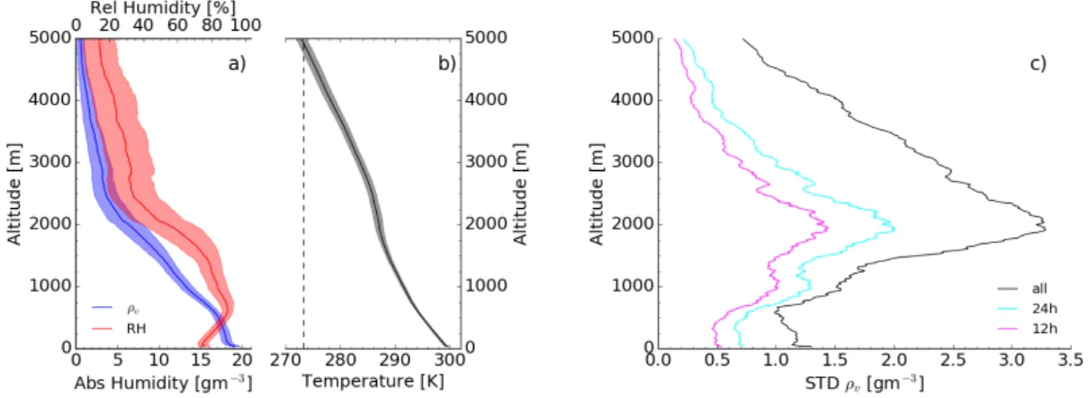
and 200 GHz . . . 18 3.1 Barbados Cloud Observatory in February 2019 . . . 26 3.2 Mean and variability of humidity and temperature profiles measured

by ascending soundings launched at BCO during EUREC

⁴

A . . . 30 4.1 Concept, instruments and their observations used in the synergistic

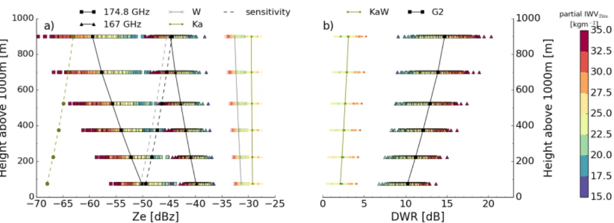
retrieval approach . . . 44 4.2 Radar reflectivity and DWR simulated for 633 atmospheric profiles

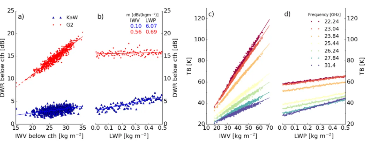
with single cloud layer based on soundings launched at Barbados . . . 49 4.3 Simulated DWR and TB as function of water vapor and liquid water

conditions . . . 50 4.4 Retrieved profile and uncertainty for case study on 19.02.19, 10:46

UTC using synergistic and standalone retrieval configuration . . . 52 4.5 Relative DFS gain to MWR-only retrieval of the case study retrieved

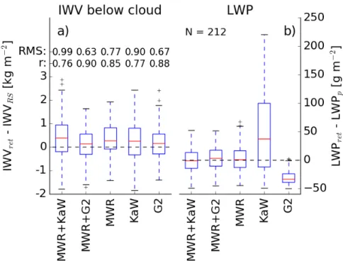
profiles . . . 54 4.6 Difference between retrieved partial IWV to sounding partial IWV,

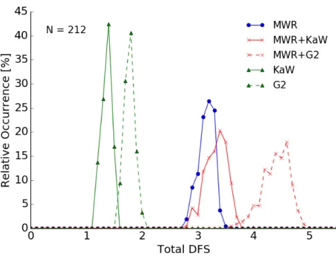
and retrieved LWP to assumed LWP for all different retrieval setups . 57 4.7 Frequency of occurrence of total DFS for 212 converging retrieved

cases in all different retrieval configurations . . . 58 4.8 Mean DFS, vertically cumulated and depicted per retrieval state for

212 converging cases in all retrieval configurations . . . 59

vii

(8)

viii List of Figures

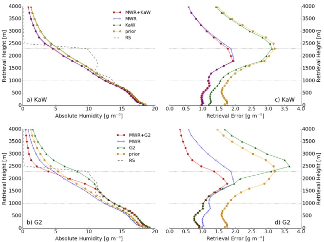
4.9 Mean a posteriori retrieval error of retrieved absolute humidity per retrieval grid step for 212 converging cases in all retrieval configurations 60 4.10 Mean synergistic a posteriori retrieval error for synergistic MWR+G2

retrieval for varying measurement and prior errors as well as radar sensitivity thresholds . . . 62 5.1 Aqua MODIS composites of area around Barbados on 10., 11., 13.02.20 68 5.2 Sounding profile, as well as real and simulated radar and MWR

observations at BCO on 10.02.20, 10:46 UTC . . . 70 5.3 Sounding profile, as well as real and simulated radar and MWR

observations at BCO on 12.02.20, 02:47 UTC . . . 71 5.4 Sounding profile, as well as real and simulated radar and MWR

observations at BCO on 13.02.20, 22:52 UTC . . . 72 5.5 Correlation matrix derived from climatology of soundings launched at

Grantley Adams International Airport, Barbados . . . 74 5.6 Case 1, 10.02.20, 10:46 UTC: Retrieved profiles, optimal to prior

uncertainty ratio and DFS . . . 75 5.7 Case 1, 10.02.20, 10:46 UTC: Retrieval DFS and partial water vapor

amount . . . 75 5.8 Case 2, 12.02.20, 02:47 UTC: Retrieved profiles, optimal to prior

uncertainty ratio and DFS . . . 77 5.9 Case 2, 12.02.20, 02:47 UTC: Retrieval DFS and partial water vapor

amount . . . 77 5.10 Case 3, 13.02.20, 22:52 UTC: Retrieved profiles, optimal to prior

uncertainty ratio and DFS . . . 78 5.11 Case 3, 13.02.20, 22:52 UTC: Retrieval DFS and partial water vapor

amount . . . 78 5.12 Correlation matrix derived from error covariances of the temporal

interpolation at 12 hours between 24-hour spaced operational soundings 81 5.13 Reconstructing the water vapor profile between 24-hour spaced

soundings: Retrieved absolute humidity profiles, optimal to prior uncertainty ratio and DFS for three EUREC

⁴

A cases . . . 82 5.14 Reconstructing the water vapor profile between 24-hour spaced

soundings: Retrieval DFS and partial water vapor amount for three

EUREC

⁴

A cases . . . 84

(9)

List of Figures ix 5.15 Expanding the concept by synthetic Raman lidar observations:

Retrieved absolute humidity profiles, optimal to prior uncertainty ratio and DFS for three EUREC

⁴

A cases . . . 87 5.16 Expanding the concept by synthetic Raman lidar observations: Partial

and total DFS and water vapor amounts for three EUREC

⁴

A cases . 88 5.17 Expanding the concept by synthetic Raman lidar observations: Case

1, 10.02.20, sensitivity to Raman lidar measurement error . . . 89 5.18 Modifying the retrieval setup: Case 2, 12.02.20, retrieved profiles,

optimal to prior uncertainty ratio and DFS . . . 92 5.19 Mean and standard deviation profile of absolute humidity measurements

for low or high IWV and ρ

_2m

conditions . . . 96 6.1 Sounding humidity profiles and simulated airborne measurements for

selected EUREC

⁴

A cases 10., 12., 13.02.20 . . . 102 6.2 Cloudnet cloud target classification at Ny-Ålesund, 08.03.2017 . . . . 105 6.3 Humidity and temperature profile of sounding launched at Ny-Ålesund,

08.03.2017, 12 UT . . . 106 6.4 Sounding humidity profiles and simulated radar measurements for

mixed-phase cloud scenario at Ny-Ålesund, 08.03.2017, 10:46 UTC . . 107

(10)

(11)

List of Tables

4.1 Characteristics of considered observations . . . 46 4.2 Case study DFS for different retrieval setups: synergistic approach

with MWR and dual-frequency radar observations, MWR-only configuration, and dual-frequency radar-only . . . 54 4.3 Mean DFS for 212 cases converging in all varying retrieval

configurations using MWR and KaW or DAR G2 observations . . . . 59 4.4 Mean DFS of MWR+G2 retrieval for different radar sensitivity thresholds 63 5.1 Climatological Sounding Prior: Gain of synergy DFS compared to the

MWR-only and DAR-only configuration, as well as error reduction compared to the MWR-only configuration . . . 79 5.2 Reconstructing the atmospheric state between 24-hour spaced

soundings: Gain of synergy DFS compared to the MWR-only and DAR-only configuration, as well as error reduction compared to the MWR-only configuration . . . 83 5.3 Expanding the concept by synthetic Raman lidar observations: Gain

of synergy DFS and optimal to prior uncertainty ratio reduction compared to the MWR+G2 configuration . . . 86 5.4 Retrieval configurations to evaluate information optimization above

each cloud layer . . . 91

xi

(12)

(13)

1 Introduction

1.1 Scientific Motivation

Water Vapor and Cloud Observations Throughout the Centuries

Weather phenomena, clouds, and water vapor have fascinated and served as inspiration for generations of scientists, artists, writers, and dreamers. While weather observations can be traced back to civilizations as early as the Babylonians and several ancient peoples in India, the earliest conveyed essay known to date summarizing the state of the art of atmospheric knowledge is Aristotle’s De Meteorologica , written around 340 BC (Frisinger, 1972). Clouds and water vapor play a fundamental role in Aristotle’s theories and observations, as he describes the cycle of evaporating water forming clouds from which precipitating liquid or ice closes what now is referred to as the hydrological cycle

¹

.

Aristotle’s work on meteorology shaped western thinking about meteorology until the 17

^th

century, when scientists like Galileo and Pascal designed first scientific experiments to understand nature phenomena, as opposed to the observation-based scientific thinking that dominated the centuries before (Frisinger, 1973). In the 18

^th

and 19

^th

century, fundamental processes were discovered in pioneering experiments regarding basic physical laws in thermodynamics and astronomy. For example, in 1856, Foote (1856) first discovered that water vapor and CO

2

could absorb and emit heat, leading to warming effects in the atmosphere. Tyndall further specified in 1859 that specifically longwave infrared radiation caused the warming effect (Tyndall, 1859); see also Hulme (2009) and Jackson (2020). Arrhenius (1896) found that emitting CO

2

to the Earth’s atmosphere would lead to increasing surface temperatures. The role of clouds in influencing the Earth’s radiation budget was first noted by Abbott and Fowle (1908).

1

Translation of Aristotle’s

De Meteorologica

available by Webster (2020); the cycle between clouds and precipitation is mentioned in book 1, part 9; and book 2, part 2.

1

(14)

2 Introduction

Since initial measurements documenting increasing atmospheric CO

2

concentrations (Keeling, 1960), scientists have warned of the implications of increasing CO

2

emissions leading to a globally changing climate (Charney et al., 1979) and major efforts have been undertaken to understand the present climate system and evaluate future, changing climate scenarios. The Intergovernmental Panel on Climate Change (IPCC) therefore assesses the current state of changing climate regularly, evaluating observations and models (current report: IPCC (2013), next one expected for 2021).

Since General Circulation Models (GCM) have emerged as a tool to model current and predict future global climate scenarios (e.g. Smagorinsky, 1963), modeling and forecasting capacities have tremendously improved over the past decades (Bauer et al., 2015). Yet, uncertainties remain, for example due to the characterisation and parametrisation of feedback processes that amplify or dampen the response of the climate system to forcing (Hansen et al., 1984; Held and Soden, 2000; Bony et al., 2006, most recent review: Sherwood et al. (2020)). Processes related to water vapor show large positive feedback throughout models (Held and Soden, 2006), while the role and magnitude of cloud feedback has been known as very important, but not yet clearly quantified in its magnitude (Cess et al., 1990; Hartmann et al., 1992;

Stephens, 2005; Boucher et al., 2013). Subgrid-scale processes driving water vapor and cloud feedback are not resolved in GCM models, but rely on parametrisation schemes (e.g. Tiedtke, 1989; Arakawa, 2004; Jakob, 2010).

Water Vapor Structure and Shallow Clouds in the Trades

In particular, the representation of low tropical marine boundary layer clouds in the subtropical subsidence zones leads to major inter-model spreads (Bony and Dufresne, 2005; Dufresne and Bony, 2008; Nuijens and Siebesma, 2019). These clouds are small in size and ubiquitous over the tropical oceans. At Barbados, shallow maritime cumulus clouds can be observed year-round, and they are representative for tropical marine boundary-layer clouds (Medeiros and Nuijens, 2016).

The clouds and structure of the trade wind driven atmosphere have been of interest since the first coordinated observation periods of the Northern Atlantic trades (e.g.

Malkus, 1958). Characterized by strong surface easterlies, the trade winds, the

vertical moist structure is characterized by a moist convective layer, a transition

zone characterized by the typical increase of temperature ("trade inversion") with

an associated strong moisture gradient ("hydrolapse"), and the dry free troposphere

resting above the trade inversion (see Fig. 1.1). The lower structure of the moist layer

(15)

1.1 Scientific Motivation 3

Figure 1.1

– Structure of water vapor and clouds in the (sub-)tropics, adapted from Stevens et al. (2017). The sub-cloud layer is limited by the LCL, while shallow clouds between LCL and the trade inversion height. The lower free troposphere ranges between trade inversion and freezing level below the dry free troposphere. The Barbados Cloud Observatory is located in the sub-tropical subsidence zone.

is marked by a well-mixed sub-cloud layer, driven by evaporation and turbulences (e.g. Betts and Albrecht, 1987). The convective potential of the moist layer is determined by the water vapor amount in the sub-cloud layer (e.g. Stevens et al., 2017). The Lifting Condensation Level (LCL) varies little over time and, at Barbados, is usually located between 600 m to 800 m (Nuijens et al., 2014; Stevens et al., 2017).

Cumulus clouds form between LCL and the trade inversion layer (ranging around 2000 m ), transporting and distributing water vapor vertically. Clouds appear as shallow cumulus humilis clouds, and can grow to large towers of cumulus congestus, often sheared horizontally due to strong winds, sometimes pushing through the trade inversion, transporting moist air into the dry lower free tropospheric environment.

Vertical cloud development is capped by the trade inversion. Therefore, moisture is trapped below the inversion, and stratiform cloud outflow layers can form (e.g.

Lock, 2009). Recent observational studies found that the highest variability of

cloud fraction is observed around LCL and around the stratiform outflow below the

trade inversion (Nuijens et al., 2015; Brueck et al., 2015; Lamer et al., 2015). The

dry free troposphere is characterized by dry air, often characterized by large-scale

subsidence. This air originates from the Intertropical Convergence Zone (ITCZ),

and is transported polewards by the Hadley circulation. Varying on the circulation

conditions, elevated moisture layers can be advected to the trade wind driven regions

often associated with altocumulus or -stratus clouds, or Saharan dust layers impacting

the radiative heating profiles (Gutleben et al., 2019).

(16)

4 Introduction

The moisture structure is driven by moist convective processes that are closely intertwined with cloud and circulation processes (Derbyshire et al., 2004; Stevens, 2004; Sherwood et al., 2010). Local convective processes and shallow cloud formation interact with their immediate local environment e.g. through entrainment or precipitation, but interplay with large-scale circulations (e.g. Riehl and Malkus, 1957;

Nuijens and Siebesma, 2019). Mesoscale convective aggregation and organization further affect the cloud and water vapor distribution (Bretherton et al., 2005; Tobin et al., 2012; Holloway et al., 2017). Not only is the amount of water vapor important for clouds and convection and, thus, feedback processes, but also is its distribution and variability.

The structure of lower-tropospheric water vapor mixing and moisture transport are crucial for determining low cloud feedback processes (Sherwood et al., 2014).

Convective precipitation amounts strongly relate to the total vertical moisture content, but particularly to water vapor variability in the lower troposphere above LCL (e.g. Bretherton et al., 2004; Holloway and Neelin, 2009; Nuijens et al., 2009;

Stevens et al., 2017). The variability of tropospheric water vapor amount is largest around cloud base (Stevens et al., 2001), where it influences the cloud amount and, thus, low cloud feedback processes (e.g. Brient et al., 2016; Vial et al., 2017).

Important water vapor feedback processes result from radiative cooling. A substantial enhancement of cooling can be induced by water vapor variations in the dry subsiding free troposphere (e.g. Pierrehumbert, 1995; Spencer and Braswell, 1997; Gutleben et al., 2019). Variations in the moist layer can lead to the formation of cold pools, which further enhance cooling and drive circulation patterns (Zuidema et al., 2012b).

Shallow Clouds, Convection and Circulation

Yet fundamental questions remain unanswered for a thorough understanding of

how shallow clouds and related convection and circulation processes will change

in a changing climate (e.g. Stevens and Bony, 2013; Bony et al., 2006; Marotzke

et al., 2017). While it is generally acknowledged that water vapor amounts in

the troposphere increase with warming temperatures (Trenberth et al., 2005), it

is not clear whether increasing temperature will lead to a reduction of low-level

clouds and thus amplify warming (e.g. Rieck et al., 2012; Webb and Lock, 2013), or

whether increasing Sea Surface Temperature (SST) will lead to an increase of low

cloudiness due to enhanced clear-sky radiative cooling and convection (Wyant et al.,

2009). Which cloud-controlling processes will be dominant in a warming climate

(17)

1.1 Scientific Motivation 5 under different future radiative forcing scenarios (Bretherton et al., 2013)? How do moisture mixing processes in the lower troposphere influence cloud feedback, and how will mixing processes change in a warming climate (Sherwood et al., 2014)?

Which processes and their representation through parametrization are particularly responsible for the discrepancy between observed and modeled tropospheric water vapor mixing and amounts (Pierce et al., 2006; Bony et al., 2015)?

Field Study Observations in the Northern Atlantic Trades

In order to shine a light on these questions, to improve the understanding of underlying feedback, and in order to evaluate parametrization schemes, thorough observations of the interplay of convection, clouds, and large-scale circulation are crucial in areas with prevailing shallow clouds, such as the trades. The trades and their clouds have been of scientific interest since the pioneering landmark studies by J.

Malkus and H. Riehl (Riehl and Malkus, 1957; Malkus, 1958). Airborne observations during BOMEX ( Barbados Oceanographic and Meteorological EXperiment ; Holland, 1970; Friedman et al., 1970), as well as shipborne measurements during ATEX ( Atlantic Trade-Wind EXperiment ; Augstein et al., 1974) increased the observational understanding significantly, and provided observational data for many modeling studies (e.g. Stevens et al., 2001).

While the Rain In shallow Cumulus over the Ocean -experiment (RICO; e.g.

Rauber et al., 2007; Davison et al., 2013) targeted measurements of key processes around precipitation, the Barbados Aerosol Cloud EXperiment BACEX (Jung et al., 2016) and the CARRIBA-project ( Cloud, Aerosol, Radiation and tuRbulence in the trade wInd regime over BArbados , Siebert et al., 2013) focused on aerosol-cloud-precipitation interaction. More recently, the interplay of clouds, convection and circulation was further studied during the NARVAL field studies, in which the research aircraft HALO was equipped as a cloud observatory (Stevens et al., 2019). The measurements build the foundation for characterizing cloud properties (e.g.

Schnitt et al., 2017; Jacob et al., 2019), water vapor structure (Naumann and Kiemle,

2020) and large-scale convergence (Bony and Stevens, 2019). The EUREC

⁴

A (Bony

et al., 2017; Stevens et al., 2020a) field study took place in 2020 to further elucidate

the couplings between clouds, convection, and circulation, including interaction with

the ocean surface and eddies, respectively. The coordinated measurements of four

research aircraft and four research ships were complemented by a high temporal

resolution upper air sounding network (Stephan et al., 2020, and Sec. A.1), high

(18)

6 Introduction

temporal resolution dropsonde activity, and intensive remote sensing and in-situ observations.

Global Radiosonde Network

While intensive periods of observations during field studies offer valuable testbeds for model parametrization development and evaluation, as well as process understanding of interplay between small- and large-scale environments, long-term stationary observations are crucial for observing trends on longer time scales (Wulfmeyer et al., 2015). In the tropics, long-term observations are mainly available from radiosondes and spaceborne remote sensing observations. Launched within a globally connected network every 6, 12, or 24 hours, regular radiosonde launches at coordinated times worldwide are a crucial pillar of global atmospheric observations. Each sounding is timed such that it reaches the 100 hPa -level at coordinated UT times, generally at 00, 06, 12, or 18 UT . At Barbados, soundings have been launched every 12 or 24 hours from Grantley Adams International Airport (GAIA, station identifier: TBPB) for the 00 and 12 UT times since 1973.

Equipped with a humidity, temperature, and GPS-sensor, modern soundings record vertical profiles of temperature, humidity, pressure, wind speed and direction, as well as position and altitude. Sounding measurements can be affected e.g. by solar radiation, varying with pressure level and sun elevation; by different sensor response times, varying with pressure; by sensor icing and wetness when ascending through cloud layers; and by horizontal drifting depending on the wind conditions. Different correction algorithms need to be applied depending on the type of radiosonde used (Vömel et al., 2007; Turner et al., 2003; WMO et al., 2011). Challenges in the analysis of longterm trends or re-analysis data are introduced by different sounding types used worldwide and over time, and by differently strong horizontal drifting depending on the launch location (Finger and Schmidlin, 1991; Ross and Elliott, 2001; Durre et al., 2006).

Satellite Observations

Even though satellite observations cannot reach the vertical resolution that soundings provide, observations are available with broad global coverage, particularly providing measurements over remote, inaccessible regions of the world. Long records, e.g.

by the Special Sensor Microwave Imager/(Sounder) (SSMI/(S)) instrument on the

(19)

1.1 Scientific Motivation 7 Defense Meteorological Satellite Program (DMSP) satellites, in space since 1978, help to diagnose worldwide trends and observations of water vapor conditions under changing climate (e.g. Schulz et al., 1993). Longterm trends can be analyzed once the biases between the different sensors are corrected for (Trenberth et al., 2005;

Sohn and Smith, 2003), and can be used to evaluate water vapor representation in climate models (e.g. Chen et al., 1996; Pierce et al., 2006).

Since data assimilation procedures have moved forward to 4D-var algorithms, the humidity observations over oceans provided by microwave satellite sounders such as SSMI/S or the Microwave Humidity Sounder (MHS) have been significantly improving forecasts up to multiple days (e.g. Geer et al., 2017). Recent efforts have been made to include more satellite radiances into all-sky data assimilation (Geer et al., 2019) for ECMWF forecasts and re-analyses. Boundary layer moisture structure is a key to successful assimilation strategies, particularly in the tropics, and requires bias free observations for model evaluation (Andersson et al., 2007).

However, while low revisiting times of twice per day in case of polar orbiters prohibit the quantification of short-term processes, instruments on geostationary orbits with higher temporal resolution operate in the visible or infrared, but cannot penetrate clouds (e.g. Wulfmeyer et al., 2015, for overview). Humidity observations are therefore only available above the highest cloud layer, and large portions of the available water vapor in the boundary-layer are missed in the presence of clouds. Microwave sounders like the Advanced Microwave Sounding Units (AMSU)-A or -B can penetrate clouds, but suffer from low vertical resolutions due to broadening weighting functions towards the lower troposphere where highest water vapor amounts and variability are expected in the trades. Often, satellite footprints are larger than the actual observed clouds.

Active remote sensing instruments on satellites forming the A-Train like CloudSat

(Stephens et al., 2002) and the Cloud-Aerosol Lidar and Infrared Pathfinder Satellite

Observations (CALIPSO Winker et al., 2010) complement the picture of passive

sensors. Spaceborne lidar observations by CALIOP (Cloud-Aerosol Lidar with

Orthogonal Polarization,) on CALIPSO, and the Cloud Profiling Radar on CloudSat,

offer high vertical resolution, and advance the monitoring of the vertical structure

and properties of clouds and aerosols (Stephens et al., 2018). Yet the detection of

shallow maritime clouds is challenged by radar instrument sensitivities (Lamer et al.,

2020). Spaceborne water vapor profile observations can be advanced by combining

active and passive instruments on one satellite, such as is planned for the future

EarthCARE mission (Illingworth et al., 2015b).

(20)

8 Introduction

Ground-based Remote Sensing Observatories

Even though spaceborne remote sensing applications cover a larger area than radiosondes and can capture large-scale conditions, the characterization of water vapor and cloud interplay requires a higher horizontal, vertical, and temporal resolution than what is feasible with current satellite sensors (e.g. Wulfmeyer et al., 2015).

In order to overcome these observational constraints, ground-based remote sensing observatories such as the Barbados Cloud Observatory (BCO, Stevens et al., 2016) in the subtropics, or the ARM facilities (Ackerman and Stokes, 2003) and the Jülich ObservatorY of Cloud Evolution (JOYCE, Löhnert et al., 2015) located in the mid-latitudes can monitor the atmospheric column continuously. Ground-based remote sensing networks can fill observational gaps between operationally launched soundings (Löhnert et al., 2007), and can be integrated reliably into data assimilation to improve numerical weather prediction (NWP) (Illingworth et al., 2015a; Cimini et al., 2012; De Angelis et al., 2017).

While passive remote sensors capture natural thermal emissions of atmospheric constituents, active sensors transmit a beam of radiation and receive the backscattered signal. In case of the radar, the transmitted signal is at microwave frequencies, and backscattering targets are cloud or precipitation hydrometeors; lidars transmit a visible or near-infrared signal, which scatters on aerosols and molecules. While remote sensing applications based on visible or infrared radiation mostly cannot penetrate clouds, microwave remote sensing like the microwave radiometer or radar can profile through cloud layers.

Microwave radiometers sense atmospheric emissions mainly originating from energy state transitions of water vapor, oxygen, and liquid water. These emissions can be expressed as brightness temperatures according to Planck’s law. By combining the brightness temperatures measured in different frequencies, the Integrated Water Vapor (IWV), Liquid Water Path (LWP), and coarse humidity and temperature profiles can be derived, given precipitation-free conditions (Westwater, 1978; Löhnert and Crewell, 2003). In order to solve the ill-posed inverse problem of linking the measured radiometric measurements to atmospheric states, multiple retrieval methods are available (Solheim et al., 1998): statistical regression retrievals (Crewell and Löhnert, 2003); physical retrievals such as the optimal estimation framework introduced by Rodgers (2000); or neural network retrievals (Cadeddu et al., 2009).

Yet, due to coarse weighting functions of the channels, the vertical resolution of the

(21)

1.1 Scientific Motivation 9 temperature and humidity profiles is limited (e.g. Güldner and Spänkuch, 2001), such that strong humidity gradients or temperature inversions are likely not resolved.

Generally, active sensors can achieve a higher vertical resolution than passive sensors. Water vapor profiles derived from lidar instruments reach vertical resolutions of a few meters in cloud-free situations given long integration times, but cannot profile the whole atmospheric column in the presence of clouds. While cloud radars, for example using Ka- or W-band frequencies, can profile through clouds with short integration times of a few seconds and single-frequency applications can deduct cloud and precipitation properties, the water vapor distribution cannot be derived.

Combining two frequencies in a differential absorption approach can overcome some of these limitations. By locating one channel in the center of an absorption line, and a second channel on its wing, the height-resolved concentration of atmospheric gases can be measured. The differential absorption principle has been used for decades using visible frequencies with lidar instruments (DIfferential Absorption Lidar (DIAL) to derive the vertical structure of water vapor (Schotland, 1966) in clear conditions or until signal saturation at cloud base. Recently, frequencies in the microwave spectrum around the 183.31 GHz (G-band) water vapor absorption line (Differential Absorption Radar (DAR); Battaglia et al., 2014; Lebsock et al., 2015) have been used to determine the water vapor profile in cloud layers in the boundary layer (Roy et al., 2020) and to assess the potential for ice cloud profiling (Battaglia and Kollias, 2019). While DIAL gives accurate profiles up to cloud base, DAR can deliver accurate humidity profiles within each cloud layer, and the partial water vapor amount between radar and the lowest cloud base. Both techniques are insensitive to the water vapor structure above the highest cloud top due to signal saturation or lack of backscattering targets.

Ground-based Sensor Synergy

In order to overcome the restrictions of each sensor, synergistic retrievals can be used

to make use of the complementary potential of different remote sensing applications

available at ground-based observatories (Stankov, 1998). In particular, the

combination of passive and active instruments is beneficial. The Cloudnet algorithm

(Illingworth et al., 2007), operational at multiple cloud observatories like JOYCE or

BCO, combines ceilometer, radar, and MWR observations to retrieve cloud boundaries

and properties, and offers a target classification product as well as thermodynamic

profiles. The integrated profiling technique (Löhnert et al., 2004, 2007) combines

(22)

10 Introduction

MWR, Ka-radar, and ceilometer in an optimal estimation approach to derive humidity, temperature, and liquid water content profiles in cloudy and drizzling conditions, as well as effective radius (Ebell et al., 2017). Barrera-Verdejo et al.

(2016) and Foth and Pospichal (2017) combine Raman lidar and MWR, enhancing the retrieval performance in clear and cloudy conditions. Combing MWR and a ground-based infrared spectrometer (Atmospheric Emitted Radiance Interferometer, AERI) decreases retrieval errors for lower tropospheric temperature and humidity profiling in clear conditions (Löhnert et al., 2009) and below cloud boundaries (Blumberg et al., 2015). A combination of ground-based MWR and spaceborne infrared (IR) instruments enhances the information content for temperature and humidity profiles in clear conditions (Ebell et al., 2013), and for IWV and atmospheric stability (Toporov and Löhnert, 2020).

Figure 1.2

– MWR (blue), Raman-Lidar (purple) and radiosonde (black) measurements of water vapor mixing ratio at BCO, 02.02.20. The sounding was launched at 10:51 UTC, and the MWR and lidar observations were averaged within a

±

2 minute window around the sounding launch. A shallow cloud formed above LCL with cloud base located at

620 m

(black dash).

However, so far, no reliable remote sensing technique exists for retrieving the whole

column water vapor profile, particularly the lower tropospheric profile, in the presence

of one or multiple cloud layers with sufficient vertical and temporal resolution (Nehrir

et al., 2017; Stevens et al., 2017; Pincus et al., 2017). This observational gap has

been identified as critical atmospheric variable for NWP by the World Meteorological

Organisation (WMO, 2014). Figure 1.2 illustrates this observational gap, based on

(23)

1.2 Research Questions and Thesis Outline 11 the remote sensing and sounding measurements at BCO for a shallow Cumulus case example during the EUREC

⁴

A campaign. The MWR-derived profile, limited by a rather coarse vertical resolution, does not resolve the sharp moisture gradients, particularly occurring around the trade inversion (on this day located at around 2300 m ). The derived profile suggests an underestimation of the moisture content in the moist layer, and an overestimation of the moisture in the free troposphere. The profile derived from the Raman-Lidar represents the conditions below the cloud layer very accurately. Above cloud base, however, no profile can be retrieved as the lidar beam cannot penetrate the liquid targets. Additionally, an accurate profile cannot be derived within the overlap region of the instrument, reaching up to 100 m . The illustrated case implies the necessity for an observational method that can profile through clouds, can continuously monitor the full atmospheric column, and can achieve a sufficiently high vertical resolution to improve the representation of the typical strong humidity gradients observed in the trades.

1.2 Research Questions and Thesis Outline

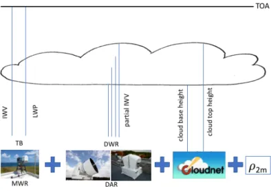
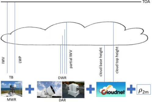
In this thesis, the potential of closing this observational gap is assessed by combining MWR and dual-frequency radar observations. The proposed instrument synergy combines the advantages of each instrument, such as sketched in Fig. 1.3: while the MWR provides information about the integrated column water vapor amount, and a coarse water vapor profile, the dual-frequency radar constrains the retrieval within the cloud layer(s), and the amount of water vapor below the lowest cloud layer. The proposed synergistic retrieval approach is further constrained by supplemental 2m absolute humidity measurements ρ

_2m

, as well as cloud boundary observations. A synergy between the two instruments offers more impact than just combining each single retrieval with another, as in a combined retrieval, information from the one instrument can be supplemented with the other instrument’s information.

In the following studies, an optimal estimation framework (Rodgers, 2000) is chosen

to analyze the synergistic benefits of MWR and dual-frequency radar based on the

retrieval uncertainties, information content expressed as Degrees of Freedom of Signal

(DFS), and retrieved profile. The passive MWR channels are selected based on the

K-band channels of the HATPRO instrument (Rose et al., 2005). The frequencies

of the dual-frequency radar are chosen for the Ka- and W-band radar, available at

ground-based observatories such as BCO or JOYCE. A second frequency combination

(24)

12 Introduction

Figure 1.3

– Concept, instruments and their observations used in the synergistic retrieval approach: MWR brightness temperature TB for IWV, LWP, coarse water vapor profile;

DWR for partial IWV quantification below cloud base and in-cloud profiling; cloud base and top height provided by e.g. Cloudnet (Illingworth et al., 2007); and

2 m

absolute humidity

ρ_2m

observations. Blue lines represent the vertical range of the instruments’

observations.

in the G-band was chosen according to the operational G-band VIPR-instrument ( Vapor In-cloud Profiling Radar , Roy et al., 2020), so far the only such instrument in operation. As no simultaneous observations are available of all instruments, synthetic observations have been generated using the Passive and Active Microwave TRAnsfer (PAMTRA) forward simulator (Mech et al., 2020) for typically observed conditions at BCO. Atmospheric profiles measured by radiosondes are combined with idealistic single- and double-layered cloud properties to generate brightness temperatures, radar reflectivities, atmospheric attenuation, and the radar differential Dual-Wavelength Ratios (DWR).

The following research questions of this thesis will be addressed in two main studies.

They will structure the potential analysis of the benefits, limitations and applicability of the proposed synergy concept in this thesis.

1. Which synergy potential is available when combining MWR with KaW and G2, respectively, analyzed for a single-cloud scenario in various moisture conditions observed in the trades? In which vertical levels is the synergy most beneficial?

2. How sensitive are the synergistic retrieval uncertainties and information content

to the assumed measurement errors, as well as radar sensitivity limits?

(25)

1.2 Research Questions and Thesis Outline 13 3. How much would an instrument synergy of MWR and DAR G2 improve the retrieval performance in zones of highest water vapor variability, shown for representative cases observed during the EUREC

⁴

A field study?

4. Does the synergistic MWR+DAR G2 retrieval improve the reconstruction of an atmospheric state between 24-hour spaced operational radiosondes compared to the temporal interpolated sounding profile, and, if so, at which heights?

5. Expanding the concept to including synthetic Raman lidar measurements, how does the retrieval benefit in the sub-cloud layer, and which modified retrieval configurations lead to an optimized performance between and above the cloud layers?

Before addressing the research questions, I will give a brief overview of the scientific background for microwave remote sensing applications for water vapor profiling in chapter 2. I will address the microwave radiative transfer theory, the underlying instrument principles of the microwave radiometer and radar, and give an overview of radar-based water vapor observation techniques. Outlining observations and the inverse method applied for the later analyses in chapter 3, I will first give an overview of the continuous remote sensing measurements at BCO (Sec. 3.1), including a brief overview of the intense observation period during the EUREC

⁴

A field study and the associated sounding network observations. Section 3.2 will then describe the concept behind the synthetically generated observations. The optimal estimation setup used to retrieve water vapor profiles from the observations will be introduced in Sec. 3.3.

In study 1, summarized in chapter 4 and published as Schnitt et al. (2020), the potential of the synergy concept will be investigated by combining MWR with the two different radar frequency pairs. Based on an idealized single-layered liquid cloud scenario, the synergistic benefits will be analyzed in different water vapor conditions guided by research question 1. Their sensitivity to measurement errors and radar reflectivity detection thresholds will be evaluated within research question 2.

Study 2, presented in chapter 5, will expand the potential analysis to more realistic

and, thus, increasingly complex atmospheric conditions as observed during the

EUREC

⁴

A campaign. Based on three case studies representing the main water vapor

structures occurring at BCO in trade wind driven conditions, the synergy of MWR

and G-band radar will be analyzed for a single-layered boundary layer cloud case,

a double-layer liquid cloud case, and for a scenario of an elevated moisture layer

associated with the formation of a higher, ice-containing altocumulus cloud layer. In

(26)

14 Introduction

Sec. 5.2, I will analyze the synergistic benefits and their vertical distribution using a standard climatological prior in the optimal estimation retrieval, discussing research question 3. The added value of the synergy to deriving the atmospheric state between 24-hour spaced operational sounding measurements will be investigated in Sec. 5.3, answering research question 4. Furthermore, the retrieval concept will be expanded to include synthetic Raman Lidar measurements in Sec. 5.4. The impacts on the sub-cloud layer retrieval, as well as tools for further optimizing the retrieval between and above the cloudy layers will be analyzed, resolving research question 5.

A first insight into the potential of extending the concept feasibility study to an

airborne application, or to the dry Arctic environment will be given in chapter 6

based on first synthetic measurements. In chapter 7, all findings will be summarized,

limitations of the study will be discussed, and concluding remarks will be given

regarding the potential for advancing ground-based water vapor profiling through a

synergy of MWR and dual-frequency radar.

(27)

2 Microwave Remote Sensing of Water Vapor and Clouds

This chapter presents a brief overview of the fundamentals regarding radiative transfer in the microwave part of the electromagnetic spectrum (Sec. 2.1), as well as the principles of operation and application examples of the remote sensing instruments used in this thesis (Sec. 2.2). More specifically, the MWR, the radar, and radar applications for water vapor profiling will be discussed.

2.1 Microwave Radiative Transfer

The following overview on radiative transfer will answer the following questions: How can radiation be quantified? Which processes alter the radiation along its ray path throughout the atmosphere? Which atmospheric constituents are mainly responsible for absorption and emission? Which scattering processes are important? Deeper insights than what is presented in the following can be found in many atmospheric science textbooks, as for example in Petty (2006), Liou (2002), and Ulaby (2014).

Radiation and Extinction

The spectral radiance B emitted by a medium at a particular frequency ν is described by Planck’s law (Eq. (2.1.1)) and is a function of the emitting body’s temperature T , the medium’s speed of light c , Planck’s constant h and the Boltzman constant k

B1

. For frequencies in the microwave spectrum, Planck’s law can be linearized by

1

speed of light

c

in air:

c= 3·10⁸m s⁻¹

; Planck’s constant h = 6.626

·10⁻³⁴J s; Boltzman constant kB= 1.38·10⁻²³J K⁻¹

.

15

(28)

16 Microwave Remote Sensing of Water Vapor and Clouds

the Rayleigh-Jeans approximation (Eq. (2.1.2)).

B(ν, T ) = 2hν

³

c

²

1 e

^{kB T}^hν

− 1 (2.1.1)

B

_RJ

(ν, T ) ≈ 2k

B

ν

²

c

²

T (2.1.2)

Planck’s law describes the radiation of a so-called blackbody medium, which describes a perfect absorbing body. According to Kirchhoff’s law, an absorbing body is also an emitting body, given it is in local thermodynamic equilibrium. In other words, a thin layer of e.g. air absorbs radiation, and also emits radiation according to Planck’s law, depending on its temperature. Yet, in reality, bodies often are not perfect absorbers or emitters. The so-called grey bodies emit only a part I(ν, T ) of the maximum possible radiation B (ν, T ) , scaled by the emissivity factor (ν) = I(ν, T )/B(ν, T ) .

When radiation propagates through the atmospheric medium, it interacts with atmospheric constituents such as gas molecules and hydrometeors. Radiation can be absorbed e.g. by molecules or hydrometeors, meaning that it stimulates an energy state transition, or it can be scattered, that is redirected in direction. All different gases’ and hydrometeors’ volume absorption and scattering coefficients β

_a

and β

_s

sum up to the volume extinction coefficient β

_e

(Eq. (2.1.3)). Each one of the volume coefficients β

_a

and β

_s

can be related to the mass absorption or scattering coefficients κ

_a

or κ

_s

by multiplying with the hydrometeor or gas density ρ . For example, the water vapor absorption coefficient β

_a^{W V}

equals to the product of water vapor mass absorption coefficient κ

^{W V}_a

and absolute humidity ρ

_v

. The mass extinction coefficient is a function of frequency ν , temperature T and pressure p

β

_e

(ν) = β

_a

(ν) + β

_s

(ν) (2.1.3)

= X

i

ρ

_i

· (κ

_a,i

+ κ

_s,i

). (2.1.4)

Beer’s law states that the initial radiation I(ν) is attenuated when propagating

through a medium (Eq. (2.1.5)) depending on the optical depth τ , that is the integral

over all extinction coefficients, or the layer’s transmissivity t(ν) (Eq. (2.1.6)). In the

microwave spectrum, the atmosphere is generally semi-transparent, which means

(29)

2.1 Microwave Radiative Transfer 17 that radiation can propagate through clouds and t(ν) is never zero.

I(s

2

) = I(s

1

) · exp ( − τ(s

1

, s

2

)) with τ (s

1

, s

2

) = Z

s2

s1

β

e

(ν)ds (2.1.5)

= I(s

₁

) · t(ν, s

₁

, s

₂

) with t(ν, s

₁

, s

₂

) = exp ( − τ(s

₁

, s

₂

)) (2.1.6) Along its propagation path ds , the initial radiation I(ν) is reduced by absorption processes to I

_a

, while temperature-dependent grey-body emissions I

_e

add up along the path. According to Kirchhoff’s law, the thermal emissions can again be quantified by Planck’s law (Eq. (2.1.1)). The transition of dI along its path through the atmosphere ds is described by the radiative transfer equation (Eq. (2.1.8)), and is in its presented form valid for a non-scattering volume ( β

e

≈ β

a

).

dI

ds = dI

_a

+ dI

_e

ds (2.1.7)

= β

a

· ( − I(ν) + B(T, ν )) (2.1.8)

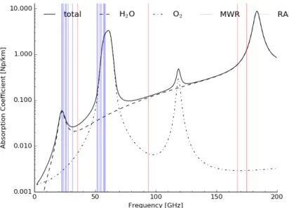
Absorption Spectrum

Absorption and emission varies throughout the microwave spectrum between 3 and

200 GHz . The main absorbing gases are water vapor and oxygen, while absorption

by other atmospheric constituents like nitrogen or ozone are of order of magnitudes

smaller. In addition to the broadened absorption lines, continuum absorption by water

vapor increases throughout the spectrum. The absorption spectrum is illustrated in

Fig. 2.1. The spectrum is characterized by the rotational absorption lines of water

vapor at 22.24 GHz (K-band) and 183.31 GHz (G-band), the oxygen absorption band

between 50 and 60.0 GHz (V-band) and at 118 GHz (F-band), as well as the increasing

absorption with increasing frequency due to water vapor continuum absorption. The

liquid water absorption increases throughout the spectrum with frequency squared

(not shown). Atmospheric pressure leads to a broadening of the respective absorption

lines as molecules are forced to collide. The absorption and, thus, also the emission

at different frequencies varies depending on temperature, humidity, and pressure.

(30)

18 Microwave Remote Sensing of Water Vapor and Clouds

Figure 2.1

– Clear air absorption spectrum for lower microwave frequency range below

200 GHz

calculated using PAMTRA (Mech et al., 2020). Water vapor (dash), oxygen (dash-dot) and total absorption (solid) were calculated at

1000 hPa

for an atmosphere with a temperature of

293.15 K

and an absolute humidity of

10 g m⁻³

. The MWR HATPRO channels are marked in red, and the used radar frequencies are marked in blue.

Scattering

In addition to absorption and emission processes, scattering also alters the radiation

on its propagation path throughout the atmosphere. The impact of scattering

depends on the radiation wavelength λ (Petty, 2006, Sec. 12.1.2), as well as the

volume- or size-equivalent radius of the scatterer r . The size parameter x = 2πr/λ

provides a first estimate about the scattering regime of the respective wavelength

used. When x 1 and assuming spherical particles, scattering processes can be

described by Rayleigh scattering (e.g. Petty, 2006), and the scattering cross section

σ

_s

is proportional to the radius of the scatterer to the power of six, and the inverse

wavelength to the power of 4. Otherwise, Mie scattering (Mie, 1908) describes the

scattering phase function of each particle, depending on the particle’s shape and

phase. σ

_s

then depends on the particular backscattering cross section σ

_bsc

. In the

lower microwave spectrum below 100 GHz , including the K-band frequencies used in

the MWR, scattering impacts of molecules or small hydrometeors are an order of

magnitude smaller than the occurring thermal emission at these frequencies. In case

of larger precipitating particles, the scattering impact can no longer be neglected

(Bobak and Ruf, 2000).

(31)

2.2 Remote Sensing Instruments 19

2.2 Remote Sensing Instruments

Emission and scattering of radiation throughout the atmosphere can be used to study water vapor and cloud properties through remote sensing instruments. Remote sensing instruments can be divided into passive and active sensors. While passive instruments receive the natural radiation I(ν) propagating through the atmosphere and altered along its path as described in Eq. (2.1.8), active sensors transmit a beam of radiation at a frequency ν and receive the back-scattered, attenuated signal.

In the following sections, the basic operational principles of the passive MWR (Sec. 2.2.1), and the active radar (Sec. 2.2.2) will be illustrated with a particular focus on applications for water vapor and cloud remote sensing. The state-of-the-art for water vapor profiling using dual-frequency radar applications will be summarized in Sec. 2.2.3.

2.2.1 Microwave Radiometer

The radiation that a zenith-pointing ground-based MWR senses in its different frequency channels can be quantified by integrating the radiate transfer equation Eq. (2.1.8) from the top of the atmosphere (TOA) to the ground as shown in Eq. (2.2.1)

I

₀

(ν) = I

_cos

· exp ( − τ) + Z

∞

0

B(ν, T (z)) · β

_a

· exp ( − Z

z

0

− β

_a

(z

⁰

)dz

⁰

)dz. (2.2.1) The overall signal I

₀

(ν) combines the initial cosmic background radiation I

_cos

= B(T = 2.7 K) , attenuated by the total column optical depth τ = R

∞

0

β

_a

dz , and the thermal emissions B(ν, T (z)) originating from each vertical atmospheric layer at height z

²

. The emitted radiation B(ν, T (z)) depends on the layer’s temperature T (z) , the gases’ and hydrometeors’ emission coefficients β

_a

(z) , and is further attenuated by the absorption between the emitting layer and the ground by the transmissivity on the way to the ground. In case of an air- or spaceborne MWR, additional radiation reflected from the ground impacts the received I(ν) .

In microwave remote sensing applications, generally the brightness temperature TB is used as opposed to the radiance I . TB describes the radiative-equivalent temperature a body would have to emit I , and can be obtained by inverting the

2

Note that

z

here refers to altitude above ground level as opposed to the radar reflectivity

z

introduced in Sec. 2.2.2.

(32)

20 Microwave Remote Sensing of Water Vapor and Clouds

Planck law or the Rayleigh-Jeans approximation (Eq. (2.1.1) or (2.1.2)). By applying inverse methods to Eq. (2.2.1), such as statistical (e.g. Westwater, 1978; Crewell and Löhnert, 2003) or physical (e.g. Rodgers, 2000; Maahn et al., 2020) retrieval algorithms, the total column water vapor amount (IWV) and the Liquid Water Path (LWP) can be quantified.

Coarsely resolved profiles of temperature and humidity can be derived from K- and V-band TBs (Güldner and Spänkuch, 2001; Liljegren et al., 2005; Crewell and Löhnert, 2007), for example available in the Humidity And Temperature PROfiler (HATPRO;

Rose et al., 2005). Accuracies of 0.8 to 1.0 g m

⁻³

(Güldner and Spänkuch, 2001) and 1.0 to 1.5 K (Crewell and Löhnert, 2007) can be reached throughout the lower troposphere in non-precipitating conditions with degrading vertical resolutions of 500 m to 1000 m . Synergies with other remote sensing instruments can further improve the retrieval performance by incorporating radar (e.g. Löhnert et al., 2004, 2008), infrared-radiometer (e.g. Löhnert et al., 2009) or lidar measurements (Barrera-Verdejo et al., 2016; Foth and Pospichal, 2017).

2.2.2 Radar

Radar instruments transmit a microwave signal and receive the radiation that is scattered back into the direction of the instrument’s antenna. Backscattering targets include cloud or precipitation droplets, ice or snow particles, birds or insects, depending on the radar’s frequency. Radars have been used for meteorological purposes since the mid-20th century, and radar theory has been summarized in many books (e.g. Battan, 1973; Rinehart, 2010; Rauber and Nesbitt, 2018).

The received power p

_r

at the radar (Eq. (2.2.2)) depends on the distance r between scattering medium and instrument, the radar reflectivity factor z

³

, as well as instrument-specific constants summarized in c

₁

. The received signal p

_r

decreases with the squared distance between radar and target

p

_r

= c

_r

z

r

²

. (2.2.2)

The radar constant c

_r

includes the radar wavelength λ , the beam’s volume described by the horizontal and vertical beamwidth θ and φ respectively, the gain factor g and the transmitted power p

_t

.

3

Reflectivity factor will be referred to as reflectivity in the following.

(33)

2.2 Remote Sensing Instruments 21 For spherical particles in Rayleigh-scattering regime, the radar reflectivity z can be described by Eq. (2.2.3), or by Eq. (2.2.4). Depending on the representation used, z thus depends on the particle size distribution N (D) and the scatterer’s diameter D to the power of six for Rayleigh scattering mediums; or, more generally, on the summarized volume backscattering coefficient of the target η = P

σ

_i

, the medium’s dielectric factor |K|

²

≈ 0.93 for liquid targets, and the radar wavelength λ to the power of four.

z = Z

∞

0

N (D)D

⁶

dD (2.2.3)

= ηλ

⁴

π

⁵

| K |

²

(2.2.4)

As the particle size distributions in clouds are wide, z spans a wide range of numbers and is therefore generally converted to logarithmic units using Eq. (2.2.5).

The equivalent logarithmic reflectivity, that is the reflectivity for equivalent spherical particles, is the un-attenuated reflectivity Z

_e^th

expected purely from scattering processes (Eq. (2.2.6)).

Z

_e^th

[dBz] = 10 log

10

z (2.2.5)

= P

_r

[dBm] + 10 log

10

(r) + log

10

(c) (2.2.6) Yet, in reality, the radar beam experiences further attenuation on its path through the atmosphere according to Beer’s law (Eq. (2.1.6)). Therefore, the measured attenuated reflectivity z

^att_e

can be calculated (Eq. (2.2.7)) by introducing the additional two-way attenuation factor T (ν, r) = 2 · t(ν, r) , specific to the radar’s frequency and range (Eq. (2.2.7), also see Lhermitte, 1990). The height-specific transmissivity t(ν) depends on the extinction coefficients β

_a

of the respective absorbing gases and hydrometeors (see Sec. 2.1), and the specific frequency (see Fig. 2.1). The logarithmic reflectivity signal Z

_e^th

is reduced to Z

_e^att

by the corresponding logarithmic transmissivity.

z

^att_e

= T (ν, r) · z (2.2.7)

Z

_e^att

= Z

_e^th

− log

10

T (ν, r) (2.2.8)

(34)

22 Microwave Remote Sensing of Water Vapor and Clouds

For simplicity, all future mentioned z

e

or Z

e

will refer to the attenuated signal without additional specification.

Most cloud and precipitation radars operate in window frequencies away from the main absorption lines to minimize signal attenuation. With increasing operation frequency, e.g. from Ka-band to W-band radar, the sensitivity to smaller particles increases, and smaller cloud droplets can be detected. Yet, also the attenuation increases with increasing frequency due to increasing absorption of water vapor continuum and liquid water. At ground-based remote sensing observatories such as BCO or JOYCE, pulsed (e.g. Görsdorf et al., 2015) and Frequency-Modulated Continuous Wave (FMCW) radars (e.g. Küchler et al., 2017) are in operation.

2.2.3 Radar Strategies for Water Vapor Profiling

Radar measurements cannot only be used to derive cloud and precipitation properties, but can also be used to measure partial water vapor amounts between adjacent radar range gates. Fabry et al. (1997) propose to use S-band radar phase information from natural ground targets to infer the refractive index of the surrounding, horizontal atmosphere, linked to the 2D-structure of temperature and moisture around the radar.

Ellis and Vivekanandan (2010) compare non-attenuated S-band with attenuated Ka-band radar measurements to derive the total water vapor attenuation at Ka-band along the ray path. Through scanning techniques, they successfully derive a low-tropospheric humidity profile with a 2 % to 6 % relative error compared to sounding in-situ measurements. Airborne return signals of a Ku- and W-band combination are used by Tian et al. (2007) to infer water vapor attenuation in a light rain field. Meneghini et al. (2005) explore the feasibility of deriving water vapor profiles based on three frequencies around the 22 GHz absorption line.

Differential Absorption Radar

Only recently, Lebsock et al. (2015) proposed a dual-frequency combination of radar

frequencies along the wing of the strong water vapor absorption line at 183.31 GHz

to derive water vapor profiles based on differential reflectivity signals. By placing

one frequency close, and one frequency further away from the line center ( online

and offline ), the Differential Absorption Radar (DAR) technique can be related to

the water vapor concentration, similarly to the DIAL technique, but is applicable in

(35)

2.2 Remote Sensing Instruments 23 cloudy situations. This technique can be used to study e.g. the boundary layer water vapor structure (Millán et al., 2016; Roy et al., 2018), or water vapor throughout ice clouds (Battaglia and Kollias, 2019).

The Dual-Wavelength Ratio (DWR) at distance r , that is the differential reflectivity signal in the corresponding range gate, can be determined by the ratio of the attenuated linear reflectivities z

_e

(ν

₁

, r) and z

_e

(ν

₂

, r) for the off- and online frequency, respectively, or the difference between the corresponding logarithmic reflectivities (Eq. (2.2.9))

⁴

. Assuming that the difference between off- and on-line un-attenuated z

_e

(Eq. (2.2.4)) is small, and that no differential scattering occurs, DWR (Eq. (2.2.9)) simplifies to Eq. (2.2.10), the ratio of transmissivities at the corresponding frequencies and range gates. Due to the strong water vapor absorption along the 183.31 GHz -line, it is valid to assume that the water vapor absorption is on order of magnitudes higher than the liquid hydrometeor attenuation. Using Eq. (2.1.6) to calculate the 2-way transmissivity, the resulting DWR signal then only depends on the water vapor specific properties as seen in Eq. (2.2.11). The differential DWR signal relates to the layer’s water vapor concentration ρ

v

, assumed constant in the respective volume, as well as the water vapor mass absorption coefficients κ

v

at the two respective frequencies (also see Eq. (2.1.4)).

DWR (ν

₁

, ν

₂

, r) = z

_e^offline

(ν

₁

, r)

z

_e^online

(ν

₂

, r) = Z

_e^offline

(ν

₁

, r) − Z

_e^online

(ν

₂

, r) (2.2.9)

= T (ν

₁

, r)

T (ν

₂

, r) (2.2.10)

= exp ( − 2 · Z

r

r0

[ρ

_v

(r) · (κ

_v

(ν

₁

, r) − κ

_v

(ν

₂

, r))]dr) (2.2.11) Profiles of partial water vapor can be inferred throughout cloud layers in-between adjacent range gates r

₀

and r , with the vertical resolution depending on the radar range gate spacing and signal processing. Additionally, the partial water vapor amount between the instrument’s location and the first backscattering target along the beam path can be derived. In a ground-based application, this partial water vapor amount could be the sub-cloud layer water vapor amount. In an air- or spaceborne application, the ground return signal can be used to derive the full-column water vapor in clear-sky conditions, the boundary layer water vapor amount below the

4

Equations have been summarized using the notation in Lebsock et al. (2015), as well as the

derivation in Roy et al. (2018) and Battaglia and Kollias (2019).

(36)

Advancing Ground-Based Water Vapor Profiling through