How Sperm Beat and Swim

How Sperm Beat and Swim

From Filament Deformation to Activity

I n a u g u r a l – D i s s e r t a t i o n

zur

Erlangung des Doktorgrades

der Mathematisch-Naturwissenschaftlichen Fakult¨ at der Universit¨ at zu K¨ oln

vorgelegt von

Guglielmo Saggiorato aus Noventa Vicentina, Italien

J¨ ulich

2016

Tag der m¨ undlichen Pr¨ ufung: 30

October 2015

It is by logic that we prove, but by intuition that we discover.

To know how to criticize is good, to know how to create is better.

H . P o i n c a r ´ e

Abstract

Understanding the dynamics of microbiological swimmers is a key element on the way to discovering biological mechanisms, to develop new sophisticated bio-mimetic technologies, e.g., artificial microswimmers, and to design novel microfluidic devices, e.g., for diagnosis applications. In this work, we focus on the dynamics of micro- swimmers with a slender flexible body, for which the spermatozoon is one of the best biological representatives.

The overarching theme of our investigation is the relation between elasticity and dynamics of semiflexible filaments, their hydrodynamic interactions and active moti- on.

We first study the dynamics of one, two and three sedimenting filaments in a viscous fluid. The dynamics of a settling filament is simpler than that of the beating flagellum because it is dominated only by the passive elastic restoring force. It allows a fundamental understanding of the dynamics generated by the competition of elastic and hydrodynamic forces. At the same time, the settling dynamics is of technological importance as it may suggest, e.g., new purification techniques. We find that the settling plane of an isolated semi-flexible filament is not always stable. When the external field is strong enough, the system encounters two (subsequent) dynamical transitions that break the planarity and chirality of the filament shape. New sta- tionary settling shapes are found that correspond to drift and helical trajectories.

Investigations with more filaments show that the settling dynamics may be much more rich than expected already at fields generated by modern centrifuges.

Sperm cells are composed of a mostly spherical head and a whip-like appendage

called flagellum. The flagellum has an oscillatory movement that sustains a traveling

wave from the head to the tail. The motion of the flagellum provides the thrust

needed to propel the spermatozoon and generates a complex flow field. As an essential

with researchers at the research center CAESAR, Bonn) and develop a minimal model of realistic beating. We infer the flagellum internal forces and, in the future, the generated flow field. It turns out that the model needs not to be complex and not to explicitly account for the observed left-right asymmetries in the rotational motion around the pinning point. The simulation closely reproduces the flagellum tracks recorded by high-speed video-microscopy, and the appropriate parameters are, thus, estimated directly from the experimental recordings. This is a new approach to extract also forces from the observed data in addition to the kinematics, as done by other established techniques.

The inspection of high-speed recording of human spermatozoa also leads us to suggest a novel mechanism to control the swimming direction of spermatozoa via higher harmonic components of the beating frequency. The proposed mechanisms explain the usual circular trajectories by a shape anisotropy, a curved flagellum or a bent midpiece. Although it may look puzzling at first that higher beating frequency break a spatial symmetry, we show that a simple model can explain the observed behavior and match simulations with experiments.

The beating pattern is not due to a predefined sinusoidal pacemaker, as used in the previous model. Instead, it is believed that the molecular motors distributed along the flagellum reach a self-organized state that generates the required force- pattern. Different models have been proposed to explain how the beating pattern is generated by a feedback system between molecular forces and flagellum shapes;

however, explicit simulations lead to unexpected buckling instabilities. Thus, we

present a simple mathematical (and later computational) model that is not bounded

to a specific biomechanical hypothesis on the traits of the molecular motors. The

resulting model highlights the difference between different feedback responses that

couple the axoneme shape to the molecular motors forces. Among the possible

models, we choose the model with the smoothest and the most regular behavior as

we expect that, because of the variability of the biological environment and of the

resilience of spermatozoa in the most disparate conditions, any representative model

of active beating should not display ill-defined behaviors. The model is applied

to the fascinating and contemporary investigation of the active response of the

beating pattern to controlled perturbations. By numerical integration of the model,

we quantify how the beating pattern (amplitude, frequency and wave vector) is

affected by the medium viscosity and we show that it is possible to entrain the

beating frequency to an external periodic force as generated in experimental setup

or by other, surrounding, spermatozoa. This top-down approach provides a simple

reference model that allows both investigation of small scale details and investigation

of large cooperative assemblies of swimmers.

Kurzzusammenfassung

Das Verst¨andnis der Dynamik von mikrobiologischen Schwimmen ist ein Schl¨ usselelement auf dem Weg zur Entdeckung von biologischen Mechanismen, zur Entwicklung neuer anspruchsvoller biomimetischer Technologien, z.B. k¨ unstlicher Mikroschwimmer, und zur Entwicklung neuartiger mikrofluidischer Systeme, z.B. f¨ ur Diagnoseanwendungen.

Im Fokus der vorliegenden Doktorarbeit steht die Dynamik von Mikroschwimmern mit filament-artiger Form und hoher Flexbilit¨at, f¨ ur die Spermien einer der besten biologischen Vertreter sind.

Das ¨ ubergreifende Thema der Arbeit ist das Wechselspiel von Elastizit¨at und Dynamik von semiflexiblen Filamenten, deren hydrodynamische Wechselwirkungen und ihrer aktiven Bewegung.

Wir untersuchen zuerst die Dynamik von einem, zwei und drei sedimentierenden Filamenten in einer viskosen Fl¨ ussigkeit. Die Sedimentationsdynamik eines passi- ven Filaments ist einfacher als die eines schlagenden Flagellums, weil sie nur durch die passive elastische R¨ uckstellkraft bestimmt wird. Dies erm¨oglicht ein grundlegen- des Verst¨andnis der durch die Konkurrenz von elastischen und hydrodynamischen Kr¨aften erzeugten Dynamik. Gleichzeitig hat die Sedimentationsdynamik technolo- gische Bedeutung, z.B. f¨ ur neue Reinigungsmethoden kolloidaler Suspensionen. Wir zeigen, dass die Deformationsebene eines isolierten flexiblen Filaments nicht immer stabil ist. Wenn das ¨außere Feld stark genug ist, ereignen sich zwei aufeinander folgende dynamische ¨ Uberg¨ange, die die Planarit¨at und die Chiralit¨at der Filament- Deformation betreffen. Dies f¨ uhrt zu neuen station¨aren Sedimentationsformen, die Drift- und Spiraltrajektorien entsprechen. Die Untersuchung von mehreren Filamen- ten zeigt, dass die Sedimentationsdynamik vielf¨altiger ist. Die hierf¨ ur notwendigen Beschleunigungen k¨onnen von modernen Zentrifugen problemlos erzeugt werden.

Spermien bestehen aus einem kugelf¨ormigen Kopf und einem peitschen-¨ahnlichen

hin fortpflanzt. Die Bewegung des Flagellums liefert den Schub, welcher erforder- lich ist um das Spermium voran zu treiben und erzeugt außerdem ein komplexes Str¨omungsfeld. Als einen wesentlicher Schritt zum Verst¨andnis der hydrodynamischen Kooperation zwischen Spermatozoen analysieren wir experimentelle Hochgeschwin- digkeitsaufnahmen von Kopf fixierter menschlicher Spermien (in Zusammenarbeit mit Forschern vom Forschungszentrum CAESAR, Bonn) und entwickeln ein mini- males Modell f¨ ur realistische Schlagmuster des Flagellums. Daraus ergeben sich die internen Kr¨afte, und in Zukunft das erzeugte Str¨omungsfeld. Es stellt sich heraus, dass das Modell nicht allzu komplex sein muss und die beobachteten Links-Rechts- Asymmetrien in der Drehbewegung um den Fixierungspunkt nicht explizit modelliert werden m¨ ussen. Die Simulation reproduziert die Bewengung des Flagellums, die durch Hochgeschwindigkeits-Video-Mikroskopie erfasst wurde; geeignete Modell-Parameter k¨onnen somit direkt aus den experimentellen Aufnahmen abgesch¨atzt werden. Dies ist ein neues Konzept, um zus¨atzlich zur Kinematik, die mit anderen etablierten Techniken beschrieben werden kann, auch Kr¨afte aus den beobachteten Daten zu extrahieren.

Die Untersuchung der Hochgeschwindigkeitsaufnahmen menschlicher Spermato- zoen f¨ uhrt ebenfalls zur Entdeckung eines neuen Mechanismus, wie Spermien die Schwimmrichtung durch h¨ohere harmonische Komponenten der Schlagfrequenz steu- ern k¨onnen. Die bisher vorgeschlagenen Mechanismen erkl¨aren die beobachteten Kreisbahnen durch eine Formanisotropie, entweder durch ein gekr¨ ummtes Flagellum oder durch ein gebogenes Mittelst¨ uck. Obwohl es auf den ersten Blick r¨atselhaft erscheint, dass auch h¨ohere Harmonische der Schlagfrequenz die r¨aumliche Symme- trie brechen k¨onnen, erkl¨art ein einfaches Modell das beobachtete Verhalten; eine quantitative Auswertung zeigt, dass die Simulationen mit den Experimenten sehr gut ¨ ubereinstimmen.

Das Schlagmuster wird in diesem Fall nicht durch einen vordefinierten sinusf¨ormigen

Schrittmacher erzeugt, wie er im vorherigen Modell verwendet wurde. Stattdessen

wird angenommen, dass die entlang der Geißel verteilten molekularen Motoren selbst-

organisiert das erforderliche Kraftmuster erzeugen. Verschiedene Modelle wurden vor-

geschlagen, um zu erkl¨aren, wie das Schlagmuster durch ein R¨ uckkopplungssystem

zwischen aktiven molekularen Kr¨aften und der Form und Elastizit¨at des Flagellums

erzeugt wird; explizite Simulationen solcher Modelle f¨ uhren jedoch zu unerwarteten

Knickinstabilit¨aten. Daher stellen wir ein einfaches mathematisches Modell-Schema

vor, das keine spezifischen biomechanischen Hypothesen ¨ uber die Merkmale der mo-

lekularen Motoren beinhaltet. Die resultierenden Modelle betonen den Unterschied

zwischen den verschiedenen R¨ uckkopplungsmechanismen, durch die die Form des Axo-

nems mit den Kr¨aften der molekularen Motoren gekoppelt wird. Unter den m¨oglichen

Modellen w¨ahlen wir das mit dem glattesten und regelm¨assigsten Verhalten aus. Auf-

grund der Variabilit¨at der biologischen Umgebung und der Widerstandsf¨ahigkeit von

Spermien unter verschiedensten Bedingungen sollte ein repr¨asentative Modell des

aktiven Flagellenschlags kein irregul¨ares Verhaltensmuster aufweisen. Das Modell

wird dann zur Untersuchung der aktiven Regulation des Schlagmusters auf ¨außere

St¨orungen angewendet. Durch numerische Integration des Modells quantifizieren wir,

wie das Schlagmuster (Amplitude, Frequenz und Wellenvektor) durch die Viskosit¨at

des Mediums beeinflusst wird und zeigen, dass es m¨oglich ist, die Schlagfrequenz mit

einem externen periodischen Kr¨aften zu synchronisieren, wie sie in Experimenten

z.B. durch andere umgebende Spermien erzeugt werden k¨onnen. Dieser Top-down-

Ansatz liefert ein einfache Referenzmodell, das sowohl zur Untersuchung von Details

des Schlagmusters einzelner Spermien als auch zur Untersuchung des kollektiven

Verhaltens großer Schw¨arme von Mikroschwimmern geeignet ist.

Contents

1. Introduction 1

2. Filaments, Elasticity, and Hydrodynamics 9

2.1. Hydrodynamics . . . . 9

2.2. Swimming with a semi-flexible filament . . . . 12

2.3. Semi-flexible filaments . . . . 19

2.4. Coupling Hydrodynamics and Elasticity . . . . 25

2.5. Active Axonemes . . . . 27

3. Models and Methods 31 3.1. Molecular dynamics simulations . . . . 31

3.1.1. Forces . . . . 32

3.2. Data Analysis . . . . 34

3.2.1. Discussion . . . . 38

3.3. Spectrogram . . . . 40

3.4. Filament Modes . . . . 41

4. Sedimenting Filaments 43 4.1. Introduction . . . . 43

4.2. Results . . . . 46

4.2.1. Deformation and Dynamics of Single Filament . . . . 46

4.2.2. Conformations and Dynamics of Two Interacting Filaments . 48 4.2.3. Three Filaments . . . . 56

4.3. Discussion and Conclusions . . . . 58

5. Flagellar Beat of Pinned Human Sperm 61

5.1. Quantitative description of sperm beating . . . . 62

5.2. Steering with Higher Harmonics . . . . 69

5.2.1. Resistive-Force Theory . . . . 71

5.2.2. Derivation of the Net Normal Force . . . . 72

5.2.3. High-speed Microscopy of the Beat Pattern of Human Sperm 77 5.2.4. Simulations of Human Sperm . . . . 80

5.2.5. Summary . . . . 85

5.3. Dissipation and Work . . . . 86

5.4. Concluding remarks . . . . 88

6. Autonomous Flagellar Beating 91 6.1. Early Failed Attempts . . . . 92

6.2. Dynamic Ginzburg-Landau Approach . . . . 95

6.3. Linear theory . . . . 97

6.3.1. Eigenvalues and model selection . . . . 97

6.4. Nonlinear model . . . 101

6.4.1. Internal and external viscous dissipation . . . 102

6.4.2. Dynamical behavior . . . 104

6.5. Discussion . . . 107

7. Concluding Summary 109

8. Outlook 113

Appendices 115

A. Adaptive time-step Velocity-Verlet 117

Bibliography 121

Definitions

In this thesis, we discuss of biological arguments that do not belong to the background of most physicists. To clarify some common sources of confusion (at least, common for the author), we summarize in this list some of the most frequent terms that do not belong to the vocabulary of classical physics. The definitions are intentionally simplified with respect to what can be found in technical publications:

Axoneme Biomechanical structure formed of 9 double-microtubules arranged in a cylindrical conformation, some times surrounding a pair of simple microtubules.

This structure forms the core of eukaryote flagella and cilia

Cilium (Plural: Cilia) Whip-like appendages of eukaryote cells, shorter than sper- matozoa, whose periodic movement has two moments: a fast stroke and a slow recovery motion.

Eukaryote Any organism whose nucleus is membrane-bounded. Example: Parame- cium

Flagellum (Plural: Flagella) Whip-like appendage developed by certain prokaryote and eukaryote cells as sensory systems and motility mechanism. Bacterial flagella are helical filaments connected to a motor at the base. Eukaryotic flagella have a complex internal arrangements of microtubules and the shape is defined by internally modulated forces.

Motor proteins/Molecular motor “Motor proteins are enzymes that convert the

chemical energy derived from the hydrolysis of ATP into mechanical work used

to drive cell motility.”[1] There are different molecular motors depending on

the function, on the walking substrate and, even, on the walking direction.

The motors found between microtubules in the axoneme are called (Axonemal) dyneins (see Fig. 1.4).

Prokaryote Organism made of a single cell whose nucleus is not membrane-bound and lacks of mitochondria and other membrane-bound organelles. Example: E.

Coli

Sperm Mature male reproductive cell or the male gamete.

Spermatium A non-motile sperm cell.

Spermatozoon (Plural: Spermatozoa) A uniflagellar motile sperm cell.

1. Introduction

We, living and adapting the world to our needs, are integrated and surrounded by a multitude of life forms. Zoology, biology and, recently, microbiology show us how diverse forms of life developed, pushed by evolutionary forces. It is common belief that most of the life forms be tailored to fill a particular niche, balancing their use or re-use of nutrients and “free energy”, all together belonging to a network where everyone is needed.

Microorganisms are important waste recyclers that re-insert carbon and other heavier elements that cannot be synthesized by biological processes in the food chain. Their presence inside our body in a positive symbiotic interaction (digestion) or as pathogenic sources determines our daily life. The sheer importance in the ecological systems is widely recognized [2]. Acquaintance with the biological and physical aspects is vital to the understanding of our impact on such systems, to their exploitation [3], and to the development of micro-robots [4] and innovative bio-mimetic technology.

Here we focus on a tiny portion of the biophysics panorama: microswimmers;

whose foundative studies trace back to the works of Gray and Hancock [5] and of

Berg [6]. For microorganisms bigger than ≈ 1 µm active directed swimming can be an

advantage over simple diffusion [2]. Among the different microorganisms that actively

move, we will focus on those that mostly live in a fluid environment, that developed

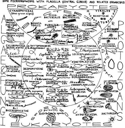
a flagellum (a whip-like appendage), and that are eukaryote. Fig. 1.1(inner circle)

shows an overview of the big variety of organisms that swim thanks to the movement

of one or many flagella. Flagella are flexible organelles that elegantly generate the

thrust with a non-reciprocal periodic motion (Fig 1.3). At these scales, indeed, a

simple periodic paddling would not generate thrust because the equation of motion

of the fluid is time-reversible and does not distinguish fast or slow strokes [7–9].

Figure 1.1.: A general overview of microorganisms with flagella and related organisms. From

Ref. [10].

1 2

4 5 6 7

9

Fibrous sheath

8 3

1 2 3 4 6 5 7 8

9

Axoneme Outer dense

f bers

Mitochondria

b

≈0.2 μm

Head Midpiece Principal piece End piece

Connecting piece Acrosome

a

c d

≈0.2 μm

≈5 μm

(human) ≈4 μm

(human) ≈50 μm

(human) ≈3 μm

(human)

Figure 1.2.: Illustration of a mammalian sperm (adapted from Ref. [14]). a) Regions of the sperm flagellum and approximate lengths. b) Cross-section of the midpiece. The microtubule doublets and associated fibers are numbered with the usual convention.

c) and d) Cross section of the principal and end pieces.

Among the flagellated eukariote microorganisms, sperm cells have a particular role, being the male gamete that is actively responsible for the ovum fertilization and, ultimately, for the organism reproduction. Sperm cells come in a variety of different shapes: some have many flagella [11], some heads are spatulate-shaped, other falciform-shaped [12], and length and size too, vary quite considerably from species to species. Indeed, one may think that spermatozoa are a mammals’ affair, but that is not the case. We are surrounded by these small cells as they are produced and released also by trees [11], insects [13] and molluscs [5]. This highlights how the sperm cells, although very diverse from species to species, are a remarkable piece of biology, adapted to very diverse and adverse environments, while still retaining their fundamental functions.

Sperm cells are not like other regular microorganisms: they do not divide nor feed or hunt; they behave more like “single-use machines”

: their life-program being simplified into “find the ovum” then “fertilize it”. From some points of view, they may seem simpler than proper organisms which need, e.g., to feed or to live in colonies, nonetheless there are still many questions to answer about their delicate taxis and

1

Thanks to Prof. B. Kaupp for this mind-opening definition.

Figure 1.3.: Left: Stroboscopic picture of a spermatozoon (sea urchin) swimming from right to left. The bright ellipse is the head, the line is the flagellum. Image from Ref. [16].

Right: High-density structures developed by sea urchin spermatozoa. The vortexes are formed by ∼ 10 cells. Image from Ref. [17].

steering mechanisms, and the ultimate influence on sperm motility and the ovum fertilization [14, 15].

In the following we consider only the case of spermatozoa: a uniflagellated sperm cell, produced by, e.g., humans, bulls and sea urchins and for this reason we employ the words sperm and sperm cells with the same meaning of spermatozoa.

The stroboscopic picture of a swimming sea urchin sperm (Fig. 1.3(left)) shows that the swimming thrust is a consequence of the bending wave that propagates downward the flagellum ( ≈ 30 − 80 µm in length and ≈ 1 − 2 µm in size, ≈ 10 − 60 Hz [2, 14]).

The flagellum pushes the cell body or head ( ≈ 5 µm) containing the highly packed DNA and some cytoplasm. The connection between cell body and flagellum differs from species to species. In the case of sea urchin the connection resembles a free joint, while in the human spermatozoon the flagellum is stiffly connected to the body. The portion of flagellum that is nearer to the body is said midpiece [12]: in the human spermatozoon, it is surrounded by mitochondria, it is then thicker and does not bend as much as the remaining length (Fig. 1.2).

The single isolated spermatozoon does not trustfully represent the swimming

conditions as sperm cells are often released in bulks. The ensuing cooperative behavior

is a very fascinating aspect of sperm motility, and a manifestation of self-organization

in nature. Theoretical and numerical investigations showed that hydrodynamics and

steric interaction lead to the formation of clusters [18, 19], similarly to other models

of self-propelled rods and spheres [20]. It is possible to describe the collective behavior also with Vicsek-like models, that means reducing each organism into few stereotyped, effective degrees of freedom. In this case the self-organization is formulated as a critical phenomenon [21]. Steric and mechanical interaction, and effective behavior are just the first guesses to describe the fascinating interactions due to the bigger number of (relevant) degrees of freedom of the real biological ensemble. Some species, indeed, developed ad-hoc features: e.g. the sperm cells of wood mouse, A. Sylvaticus, have a hook used to anchor cells in trains of cells belonging to the same male mate. Probably thanks to the hydrodynamic interaction between cells belonging to the same cluster, they travel at higher velocities than the isolated sperm and, it is believed, it strengthens the chances than one of the sperms of the cluster fertilizes the ovum [22, 23].

In Fig. 1.3 another example of cooperation is shown: when sea urchin spermatozoa (S. Droebachiensis and S. Purpuratus) swim at high density ( ≈ 2500 cells/mm

) the cells self-organize in vortexes on a hexagonal lattice [17]. The relevance of the observation is clear when the attention is shifted from models with few “effective”

degrees of freedom [21], to the actual physical and biological mechanisms of pattern formation. Depending on the context, pattern formation mechanisms may involve different processes: from the diffusion of chemical species [24–26] to advection fluxes, and (at least in ecology) non-local terms due to, e.g., roots spreading [27]. In Ref. [17]

it is proposed, for the first time, that the underlying mechanism forming the vortexes be the hydrodynamic interaction between the organisms, that couples to the flagellar dynamics thanks to some yet-unknown mechanisms.

Let’s inspect the single flagellum more carefully, then, to understand how this mech- anism may work. At the flagellum core we find the axoneme (Fig. 1.4), ≈ 0.2 − 0.5µm in diameter [1, 14], surrounded by a soft “skin” of proteins. The axoneme provides the biomechanical stability to the, otherwise soft, surrounding proteins and hosts the molecular motors [14]. The axoneme comprises 9 microtubule-doublets around a pair of central microtubules [28] and dynein arms on the outer filaments that generate shear forces between the filaments, ultimately generating the bending moments [29–

31]. The axoneme is not unique of spermatozoa as it is a highly preserved structure,

Microtubule

Microtubule doublets Radial spoke Inner-arm dynein Outer-arm dynein

Figure 1.4.: Left: Longitudinal section of two microtubules show the position and packing of the dyneins. The stalks (simple arrow) are separated by ≈ 24nm. Image from Ref. [1], Right: Illustration and cross-section of the 9+2 morphology of the axoneme (Chlamydomonas, × 218.000). The short arrow indicate the beak-like protrusion of the dynein arms. Images from Refs. [34, 36]

found also in cilia [32] and in the trypomastigote [33, 34]. Curiously, cilia are believed to form metachronal waves as consequence of hydrodynamic interaction [35], even though there are some peculiar differences with the spermatozoa.

The axoneme is the common biomechanical structure between cilia and sperma- tozoa. Since it plays a nodal role for the beating, it may be responsible for the self-organized swimming as well. The axoneme allows the generation of bending torques throughout the flagellum. It was soon realized, indeed, that since the beat- ing amplitude does not decrease at one side despite the strong dissipation of the surrounding fluid, energy must be provided all along the flagellum length [29, 37].

The mechanism generating the beat pattern drawns a lot of attention since the early works in Ref. [38]. It is well accepted that the bending forces are due to sliding forces generated between adjacent microtubules by the dynein arms (Fig. 1.4) [37–

39]. Because of the very fast beating frequency and wave velocity ( ≈ 1 mm/s), it is not possible to describe the wave as the effect of a biochemical signal. It is instead proposed that the beating pattern itself is due to a self-organization of molecular motors. Fig. 1.3 can then be seen as a self-organized motion of self-organized beating patterns!! From this point of view, the problem of active beating and self-organized swimming is a unique system to investigate physics models of interacting organisms whose behavior is not predefined but the result of the dynamics of internal degrees of freedom and external forces.

Models of active beating are then required to distinguish the effect of pure mechan-

ical forces, from active ones. Developments in the ability to manipulate and interact with the single cell [40–42], allow investigating whether cooperative behaviors can be understood as the result of mechanical forces (e.g. hydrodynamics or steric inter- action), of behavioral or signaling responses, or of others yet-unknown mechanisms.

In the latest works two main approaches have been proposed to model the beating pattern in terms of either molecular-motor traits [43–45] or mechanical properties of the filament bundle [46, 47]. But, at the moment of writing, no active model has been used to investigate the response to external perturbations.

The overarching theme of our investigation is the relation between elasticity and dynamics of semiflexible filaments, their hydrodynamic interactions and active motion.

Bearing in mind that we do not want to discuss how an idealized system reproduces the observed behaviors, but rather how a realistic system really works, we approach the investigation from different sides in the spirit of Divide et Impera.

In this thesis we initially present some original results about the hydrodynamic in- teraction of one, two and three sedimenting filaments. The dynamics of sedimentation is simpler than that of the beating, and allows developing some basic understanding on the relation between elasticity and hydrodynamic forces and on the quantification of filament shapes.

As we want to understand the hydrodynamic cooperation between spermatozoa, we focus on the design of a simulation model that closely reproduces the dynamics of a pinned (human) spermatozoa near a surface, and so the driving forces and the generated flow field. Inspection of high-speed recording of human spermatozoa led us to a new exciting observation: a novel mechanism to control the swimming direction of spermatozoa via higher harmonic components of the beating frequency.

At the same time we are left with a new minimalistic model of “realistic” beating of human spermatozoon, driven by predefined forces. Appropriate parameters are, thus, estimated directly from the experimental recordings, without micro-manipulation techniques [48].

Finally, to go beyond the predefined-forces model, we present a novel approach to

model the self-organized beating pattern. The idea is to develop a simple mesocopic

model: simple enough to be implemented in more complex simulations with full

hydrodynamics and simple enough to allow theoretical investigations on the biome- chanical structure of the axoneme. With the keen idea to start simple and generic, we have been inspired by the models of non-linear chemistry and reaction-diffusion equations [24]. The resulting framework represents an alternative approach not (yet) bounded to a specific biomechanical model of molecular motors, it highlights the dif- ference between some of the proposed models, and it allows a systematic theoretical investigation of the axonemal response to controlled perturbations

.

As always in physics, we understand a physical process via our models and theories, their underlying assumptions and limitations. In the next chapter we recall some background concepts widely used throughout this thesis:

1. Hydrodynamics at low-Reynolds number and of immersed slender objects, 2. Dynamics for semi-flexible inextensible filaments,

3. Dynamics of elastic filaments interacting with fluid, 4. Dynamics of a model axoneme.

2

Private communication with experimental groups in TU Delft and DAMTP highlighted a similar

interest, and some (very) early results with Chlamydomonas look promising.

2. Filaments, Elasticity, and Hydrodynamics

2.1. Hydrodynamics

Since we are interested in microswimmers, we are naturally concerned also of the movement of bodies in a fluid. Any movement of the immersed body propagates to elements of volume of the fluid, whose resistance itself allows the swimmer to move.

We present in this section some theoretical approaches to understand and model the equations of motion of both the fluid and the swimmer, with particular regard to slender bodies.

Navier-Stokes equation

An incompressible fluid can be described by the velocity field u, the constant density ρ and the energy k

T. The dynamics of an element of fluid in position r subject to a pressure field p and external force field f is determined by the energy and momentum conservation equation complemented with the incompressibility constrain:

ρ ∂u

∂t + u · ∇ u

= −∇ p + η ∇

u + f

(2.1)

∇ · u = 0 The first equation is the Navier-Stokes equation.

On the left-hand side of the Navier-Stokes equation the material derivative de-

scribes the acceleration and convective transport of the element of mass. Note that

the convective term is the only non-linear term. On the right-hand side the term

η ∇

u describes the momentum exchange between layers of fluid with different veloc- ities. The coupling term η is the (dynamic) viscosity: a phenomenological property of the fluid that cannot be deduced by the conservation laws. Given appropriate boundary conditions and external forces Eq. (2.1) can, in principle, be solved. They pose, however, an incredible problem that has not found a general solution yet.

Low-Reynolds number and Scallop theorem

In nature we find organisms that move in different fluids, like air or water, and at different velocity and length scales like sea whales, birds, spermatozoa, and bacteria.

We can imagine assigning a characteristic length scale L and velocity scale v

at each creature and to rescale the Navier-Stokes equation accordingly; obtaining

Re ∂u

∂t

+ u

· ∇

u

= −∇

p + η

∇

u

+ f

(2.2) where prime indicates the new dimensionless quantities.

The quantity Re = ρv

L/η is the Reynolds number: its value spans few orders of magnitude from the 10

of bacteria to the 10

of medium-size fishes [8]. Its importance resides on the fact that it defines the relative importance between the inertial forces of the fluid and the viscous forces. At high Reynolds number the motion of a body transfers momentum to the surrounding fluid, that is then convected, and slowly dissipated. On the contrary, at low Reynolds numbers there is no transport of momentum nor an inertial (delay) time between the application of the forces and the fluid response. There may be several characteristic length and velocity scales in a given system and corresponding different Reynolds number. This is not an issue as long as the Reynolds number is not confused as an absolute property of the system but, rather, of the observables of interest. For example: if one is interested on the dynamics of the single sperm cell, an appropriate choice of length and velocity can be the body length and velocity; on the contrary, if the details of fluid field near the flagellum are of interest, probably the beating amplitude and frequency provide more insight.

In this work we focus on the dynamics of the full body of spermatozoa, whose

2.1. Hydrodynamics

Reynolds number is typically small and the left-hand side of Eq. (2.2) can be neglected.

The remaining equation is called Stokes equation; it is a linear equation, with no explicit time derivative:

∇ p − η ∇

u = f

. (2.3)

Thus, the mathematical formulation of the fluid past a microorganism poses a simpler problem than that for larger creatures; however, giving away the linearity and the inertial forces affects quite a lot the physics with some counter-intuitive effects [7].

First: In this Aristotelian world all forces are instantaneously balanced [10, 49]:

when a microswimmer’s flagellum or cilia halts, the body velocity vanishes in nanosec- onds because all the momentum transfered to the fluid has been (almost) instanta- neously dissipated.

Second: Eq. (2.3) is symmetric under time inversion because the time derivative

is gone. This signifies the velocity u and pressure p fields follow instantaneously the

external force f

(t) that the swimmer imposes on the fluid. As consequence, the

dynamics for f

( − t) will be exactly the reverted dynamics. From the perspective of

a microswimmer, this really complicates life. Most of the propulsion mechanisms in

nature employ a cyclic motion, e.g. walking, flying, fish swimming are all based on

the same cyclic pattern of movements repeated over and over. The same approach

applied by a simple microswimmer with 1 d.o.f. would not work: the forces generated

in the first half cycle would balance the forces in the second half cycle. At the best, the

creature would oscillate, with no net center-of-mass displacement [50]. This is called

the “Scallop theorem” [7]. Microswimmers must have a time-irreversible propulsion

and a mechanism that involves more than one degree of freedom. From a theoretical

point-of-view the simpler of such model-swimmers can be realized with two degrees

of freedom [51]. Real microswimmers, however, developed refined and sophisticated

mechanisms. For the microswimmers we are concerned with, we highlight that ciliated

cells and sperm cells flagella actively bend their shape, and in doing so they develop

periodic patterns that break the left-right or top-bottom symmetry, thus generating

the propulsive force.

Isotropic Drag Anisotropic Drag

Figure 2.1.: Illustration of the resistive force theory applied to a rod composed of beads. The rod moves in the direction of the gray arrows. If the drag is isotropic (left) then the viscous drag (red arrows) is parallel to the velocity. An anisotropic drag (right) develops a drag force (green arrows) that is not parallel to the direction of the velocity but more oriented in the normal direction.

2.2. Swimming with a semi-flexible filament

How does the motion of an extended slender body generates the forces to self-propel in a viscous fluid? We present some theoretical concepts proposed to describe the interaction between moving slender objects in a fluid beginning with a phenomeno- logical description in the first subsection, to continue then with a more theoretical description in the following.

Resistive-force theory

Let’s consider a stiff rod of length L dragged by a force f in a viscous fluid. It moves faster when pulled along its longitudinal direction rather than when dragged along its normal direction. We can say that the friction coefficients depend on the direction the body is moving with respect to some body-axes; in the particular case of a straight rod two directions are defined (Fig. 2.1):

u

= ξ

f

Perpendicular,

u

= ξ

f

Parallel . (2.4)

2.2. Swimming with a semi-flexible filament

x

h(x,t)

t=0 t=^_

2T

+ =

Figure 2.2.: Illustration of resistive-force theory applied to a beating flagellum with period T . At the beginning (t = 0) a part of the flagellum is moving upwards (black arrow).

The flagellum is locally approximated by a rod, whose drag force (blue line) is not directed along the direction of the velocity, but it has a bigger component normal to the flagellum. A force along the x ˆ direction (red arrow) is so generated. After half a period the flagellum comes back, but because it is moving with wave-like motion, its local orientation is inverted too, and so are the forces. Nonetheless, the force component parallel x ˆ (red line) still points in the same direction and sums up to the previous one.

One of consequences of the anysotropic drag is that the drag-force is not parallel to the velocity, but it is more intense along the normal direction to the rod (Fig. 2.1).

This simple observation allows explaining how the periodic motion of the sperma- tozoon generates a net thrust: let us assume that the motion of a small segment of the flagellum (Fig. 2.2) is, essentially, along the y direction. In the absence of anisotropic drag the force in the first half period is f

= ξu

y, equal an opposite to ˆ the force generated in the second half a period f

= ξu

y ˆ = − ξu

y ˆ (Fig. 2.2, black arrows), where ξ is the drag coefficient and u

is the velocity of the small segment.

The anisotropic drag, instead, projects part of the resistance force along the positive ˆ

x direction; thus the forces generated in the two half periods have the same net contribution along the swimming direction (Fig. 2.2, red arrows).

Gray and Hancock [5] showed and verified experimentally that the swimming velocity is indeed due to the imbalance between perpendicular and parallel drag of the flagellum (Fig. 2.2):

u = − 1 2

ξ

ξ

− 1

A

ωk

1 1 + h a k/2π

, (2.5)

where the flagellum is described by a single traveling wave y(t, s) = A sin(kx − ωt)

propagating from negative to positive x, hξ

is the head drag coefficient and a the characteristic size of the head. This equation highlights few important aspects:

1. a traveling wave propagating along a slender filament can cause a net force on the microswimmer and the velocity is proportional to the drag anisotropy ξ

/ξ

− 1.

2. the force pushes in the opposite direction with respect to the wave velocity.

The sum of the forces on the fluid and on the body being, indeed, zero.

This is a very intuitive conclusion and calculations based on anisotropic drag, said “resistive-force theory”, have been successful also in describing the motion of other swimmers, e.g. E. Coli [10]. One way to measure experimentally the drag coefficients is by fitting Eq. (2.5) to the swimming velocity: for bull sperm it yields ξ

= 0.69 ± 0.62 f N sµm

and ξ

/ξ

= 1.81 ± 0.07 [52].

Thus, we have seen that a rod has two main drag coefficients and this can explain the mechanism of swimming for slender bodies. Usually, however, the coefficients ξ

and ξ

are not known for arbitrary shapes and it is natural to wonder how to estimate theoretically the perpendicular and parallel drag in complicate, possibly not-constant, shapes. In the most general case, every slender shape that moves in a fluid exerts forces the fluid itself and the effective drag-coefficient will be due to the continuously changing contributions of the distant parts of the body. In general then, it is not possible to define a “perpendicular” or “parallel” direction only. This make the problem very complicate but from a theoretical point of view, it is desirable to

“squeeze” the non-local hydrodynamic interaction to a description in terms of local

drag-coefficients. The treatment of these questions, specialized to slender objects, is

the subject of the “Slender-body theory” [10, 49, 53, 54].

2.2. Swimming with a semi-flexible filament

Stokeslets and Slender-Body Theory

The motion of a viscous fluid past a swimming microorganism of shape S(t) obeys the momentum-balance equation [8]:

∇ p − η ∇

u = 0

∇ · u = 0 . (2.6)

Usually, swimmers are impenetrable to the fluid flow, hence Eq. (2.6) is complemented with the boundary condition that the flow adheres to the surface S(t) and has the same velocity. Despite the innocent aspect of Eq. (2.6), this problem can be solved only in few lucky cases. We need an alternative approach to understand the propulsion of extended objects.

A more convenient way is to tackle the problem from the opposite point of view:

a swimmer applies forces on the fluid, whose velocity and pressure fields p and u are given by the Stokes equation. By linearity, the flow generated by any complex distribution of forces can be written as a sum of “fundamental flows” generated by point forces along the moving surface [8, 10].

The fundamental solution of Stokes equation (Eq. (2.3)) with external force given by f δ(r) and boundary condition given by zero velocity at | r | = ∞ is called

“stokeslet”. The pressure and velocity fields read:

p(r) = ∇ ·

− f 4πr

(2.7) u(r) =H(r) f , u( | r | = ∞ ) = 0

= 1

8µπr 1 + ˆ eˆ e

f (2.8)

where r = | r | is the distance from the point-force, ˆ e = r/r and H(r) is the Oseen

tensor. Eq. (2.8) shows that the velocity field is made of a component parallel to f ,

equivalent to the velocity generated by a sphere of radius r moving with the same

velocity, and a radial component given by the dyadic product that modifies the first

one with a second-order surface-harmonic [10].

We can finally write the flow field generated by a distribution of forces as super- imposition of stokeslets with force densities fδ(r(s)) along a curve whose centerline is parametrized by the curvilinear coordinate s as [8, 10]:

u(s) = f 4πµ +

Z

r(s)−r(s^′)>δ

ds

H(r(s), r(s

))f (r(s

)) (2.9) where the cut-off δ ≈

√ ea ∼ 1.36a accounts for the finite radius a of the distribution.

The general solution of Eq. (2.9) is not known, but it is readily computed for the simple case of a rod parallel to the ˆ x axis, with radius a and length L ≫ a. Each point along the filament experiences a drag force that depends its distance from the middle point:

u

(x) = f

8πµ

1 + log 4x(L − x) a

, 0, 0

u

(x) = f

8πµ

0, − 2 + 2 log 4x(L − x) a

, 0

, (2.10)

as long as x is far from the filament ends (in 0 and L). The drag coefficients are finally found integrating along the rod to obtain

ξ

= 4πµL log(L/a) + α ξ

= 2πµL

log(L/a) + β . (2.11)

Note that:

1. The constants α and β depend on the boundary conditions and the aspect-ratio.

To first order, however, they are constants: α = 0.84, β = − 0.20 [1, 50, 55]

2. Eq. (2.10) shows a logarithmic dependence on the distances from the cylinder ends. Phenomenologically, this means that the drag increases towards the ends and it is minimum at the midpoint

3. When L/a ≫ 1, the ratio between the perpendicular and parallel velocity is

almost two

2.2. Swimming with a semi-flexible filament

Instantaneous Flow Field Average Flow Field

Figure 2.3.: Instantaneous and average flow field generated by a filament moving with assigned curvature C(s, t) = C

sin(ωt + qs). Given the size and velocity of each point, the flow field is obtained from Eq. (2.9). The black points represent the filaments, the red arrows are the instantaneous local velocities and the blue lines are the stream lines.

4. In the limit of infinitely long filament, the terminal velocity diverges. This is a well know paradox. However, in practical cases one always deals with finite lengths and the problem has no relevance.

This method shows that we can, at least formally, reproduce the hydrodynamics features of extend slender object by discretizing them as spherical beads of radius a.

Concluding remarks on swimming slender bodies

Thus, we have seen that the simplification introduced by imposing a force on the fluid instead of boundary conditions allows rewriting the flow generated by a moving slender body in the simpler form of Eq. (2.9), and that using Slender-body theory and the fundamental solutions of the Stokes equation it is possible to estimate the resistive-force drag-ratios of a thin rod. For more complex objects the solution of Eq. (2.9) becomes prohibitively complicated, even more so if we consider the time- changing shape of, for example, a beating flagellum or cilium. In Fig. 2.3 we visualize the computed flow-field generated by a wave-like filament.

To overcome the difficulties introduced when applying Eq. (2.9) to biological cases,

one may be tempted to approximate the curved shape as a series of short rods. This

has the advantage of removing any non-local term, by precomputing them in the

anisotropic drag. In this way, however, the choice of the rod-length determines also

the cut-off length for the hydrodynamic interaction; the value of the rod length and

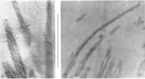
Figure 2.4.: Lateral view of cilia tips. Note the microtubule-doublets that form the axoneme.

Arrows indicate the probable ending points. From Ref. [28].

radius should not be regarded anymore as geometrical quantities, but as effective parameters that require to be fine tuned in order to reproduce the experimental data.

Interestingly, it turns out that to match the experimental data, the value of L should be replaced by the wavelength of the beating flagellum (see Ref. [5, 10, 54] for further details). A different approach is to neglect completely the Slender-body theory and to fit the swimming velocity against the drag coefficients as done in Ref. [52].

In more complex geometries, as well as in the case of interacting sperm, it is not correct to precompute the long-range terms. It is in this case that simulations really show all their power [18].

In the previous discussion of hydrodynamics at low Reynolds number and slender

bodies we implicitly assumed that the shape of the body is given. This may be the

case for some systems, but it is not the most general one. In general, bodies are

not infinitely stiff and when fluid flow exerts some forces on them, their reaction

can include a deviation from the expected shape. Before discussing this problem,

we present in the next section some theoretical models and observations on flexible

slender-bodies.

2.3. Semi-flexible filaments

2.3. Semi-flexible filaments

Polymers are ubiquitous in microbiological context: the most famous examples being DNA and proteins [56]. Recently [57], interest has grown on another class of polymer assemblies: actin, intermediate filaments, and microtubules; they are called semi- flexible filaments to highlight that the bending energy is enough to out-compete the entropic forces. Their relevant role in cellular mechanics is well accepted [1, 57, 58]:

on the contrary to the previous class of soft-polymers, this new class has a striking structural difference: they can sustain loads and exert forces. Their contribution on the formation of cellular cytoskeleton is well known, and recent investigations are highlighting their contribution to the formation many other structures, e.g. lamel- lipodia and podosomes [59, 60]. Often these biomechanical structures are not formed by a single filament alone, but by many filaments aligned in cross-connected bundles with improved stability and higher buckling threshold [57, 61].

The axoneme, clearly, belong to the category of bundles of filaments (Fig. 2.4). In this thesis we assumed that the bundles are weakly cross linked: this means that the effective bending rigidity is simply the sum of stiffnesses of individual filaments.

In the opposite case of cross-linked bundles the effective bending rigidity depends on the deformation [62]. In theoretical physics the standard model of a continuous semi-flexible polymer is the Worm-like chain [56]. In the remaining of this section we briefly present its equilibrium and dynamical traits.

When the position r(s) of the filament is parametrized by the curvilinear coordi- nate s along the filament centerline, the potential energy is readily written as the sum of two contributions: a term that penalizes the bending, and a term that penalizes the stretching [63]:

G = G

+ G

= κ 2

Z ds h

∂

r

− ∂

r · ˆ t

i + + σ

2 Z

ds [ | ∂

r | − 1]

, (2.12)

where ˆ t = ∂

r/ | ∂

r | is the unit tangent vector, κ is the bending modulus, and σ is

flexible semiflexible rod

l_p << L l_p~L l_p>>L

Figure 2.5.: Illustration of classification of polymers in terms of their persistence length at equilibrium. (Left:) The polymer is said flexible and usually modeled as a Rouse chain and thermal energy dominates the conformations. (Right:) The polymer is stiff, thermal energy is not enough to strongly affect the polymer conformation.

(Middle:) The polymer is said semi-flexible: the thermal energy and bending rigidity compete. The conformations are mostly straight, but deviations are visible.

the “stretching” modulus.

The interpretation of the potential energy is simple: the second integral vanishes when the tangent vector has velocity 1, hence when there is not stretching, the first integral vanishes when there is no bending. Note that the second contribution to the bending energy is due to the parametrization of the filament (see Ref. [63]

for a detailed explanation). Biological filaments are essentially inextensible. With a parametrization that embeds this constrain there is no need for the corresponding energy terms. Such parameterization, in 2D, is given by the curvature C(s):

r(s) = r

+ Z

0

ds

cos ψ(s

) sin ψ(s

)

!

(2.13)

where ψ(s) = R

0

ds

C(s

) is the angle between the curve and the ˆ x axis. It is easily verified that, since | ∂

r | = 1 and ∂

r = C · ˆ n, the potential energy simplifies to:

G

= κ 2

Z

ds ∂

r

. (2.14)

2.3. Semi-flexible filaments

The bending modulus can be related to the material property and geometry as:

κ = EI ∝ Ea

, [Energy × Length] (2.15) where E is the Young’s modulus, I the area moment of inertia and a the filament radius. The moment of inertia is

a

for a cylindrical section, for other sections it has different prefactors but, as long as a ≪ C

, it is always proportional to a

.

When the filament is in equilibrium with a thermal bath, the ratio between the bending modulus κ and the thermal bath energy

k

T defines the persistence length l

= κ/k

T . Intuitively, the persistence length is the length over which the polymer appears straight despite the fluctuations (Fig. 2.5):

h ˆ t(s) · ˆ t(0) i ∼ e

. (2.16) Note that the intuitive (and geometrical) interpretation has a very precise meaning only at equilibrium and for polymers whose relaxed state is straight [56]. Given the definition of the persistence length, the gyration radius reads [1]:

h R · R i = h Z

0

ds t · Z

0

ds t i = 2l

e

− 1 + L/l

. (2.17)

We move now to the introduction of basic concepts to model the dynamical behavior of semi-flexible filaments. From Eq. (2.14) we derive the equations of motion of an inextensible filament in a viscous fluid via the least-work principle [63, 64]:

∂

r =

ξ

nˆ ˆ n

+ ξ

ˆ t ˆ t

· δG

δr

= ξ

ˆ n ∂

r · n ˆ + ξ

ˆ t ∂

r · ˆ t , (2.18) where δG

/δr is the functional derivative of the potential G

with respect to the fila- ment configurations r. Eq. (2.18) has to be complemented with boundary conditions

1

k

T = 4 . 1 pN nm at 24

C .

that, for free ends read

∂

r |

= ∂

r |

= 0 . (2.19) Note that Eq. (2.18) is not linear because ˆ n and ˆ t themselves depend on the configuration r. An approximated equation in terms of small deviations from the rest state provide very useful insight. It is, in principle, possible to expand either the tangent angle or the displacement from the rest line. Let begin with the tangent angle ψ = ψ

+ ǫψ

+ ǫ

ψ

+ o(ǫ

), where ǫ is a small positive parameter. Small tangent angles correspond to an almost straight configuration, hence ψ

= 0. Substituting Eq. (2.13) in Eq. (2.18), using the fact ∂

(∂

r) = ∂

ψˆ n and collecting by equal orders in ǫ, we obtain (for the first two orders):

0 = 0+ ǫ

h

ξ

ψ

∂

ψ

+ ξ

− 3∂

ψ

∂

ψ

− 3(∂

ψ

)

i

− κ

∂

ψ = ǫξ

∂

ψ

+ ǫ

ξ

∂

ψ

.

(2.20) Expanding the configuration in small normal deviations h = (r − r

) · n ˆ [57, 64](Fig. 2.2):

r = r

+ Z

0

ds cos ψ(s) sin ψ(s)

!

ψ→0

≈ r

+ x h(x)

!

=

= r

+ x

ǫh

(x) + ǫ

h

(x) + . . .

!

. (2.21)

and inserting Eq. (2.21) in Eq. (2.18), yields:

∂

x

h

!

= − κ





ǫ

ξ

− ξ

∂

h

∂

h

ǫξ

∂

h

+ ǫ

ξ

∂

h



 (2.22)

Equations 2.20 and 2.22 highlight some important aspects of the dynamics of an elastic body in a viscous fluid:

• To first order in the deviation from the straight line, the bending energy and

2.3. Semi-flexible filaments

the perpendicular drag are the only terms that determine the dynamics,

• The inextensibility is a second order correction (see second line of Eq. (2.20)),

• Net forces along the swimming direction are generated by the second (and higher) order terms (Eq. (2.22)).

It is very instructive to spend some time on the linear dynamics, valid for “small”

deviation from the rest configuration (see also Ref. [65] for further comments.) As shown by Eq. (2.22), the dynamics of small deviations is determined by the bending energy and perpendicular drag only and Eq. (2.18) reduces to the much simpler:

ξ

∂

h = κ∂

h . (2.23)

Despite the seemingly limited range of validity, this equation is at the basis of the experimental measurement of the persistence length of biological filaments [57, 66].

Equilibrium measurements are based on the fluctuations-spectrum; indeed, a filament in equilibrium in contact with a thermal bath (ie. this means that Eq. (2.23) is complemented with white noise that satisfies the FDT theorem) fluctuates with power-spectrum:

h h

(t)h

(0) i = 2 κ

k

T L

1

q

e

(2.24)

where q = 2πn/L is the wave vector of the Fourier modes and ω(q) = κq

/ξ

. This approximation is valid when the end effects can be neglected (e.g. for fluctuations with short wavelength).

On the contrary to equilibrium measurements, it is possible to measure the per- sistence length by observing the response to controlled perturbations (see Ref. [66]

for the details). In this case it is more convenient to introduce the proper normal modes of Eq. (2.23) in dimensionless units by measuring space in units of the filament length s = Lα from the filament middle point and time in units of the relaxation time t = τ

. We obtain:

∂

h(τ, α) = ∂

h(τ, α). (2.25)

0.5 0.0 0.5 1

0 1

φ

φ

0.5 0.0 0.5

1 0 1

φ

φ

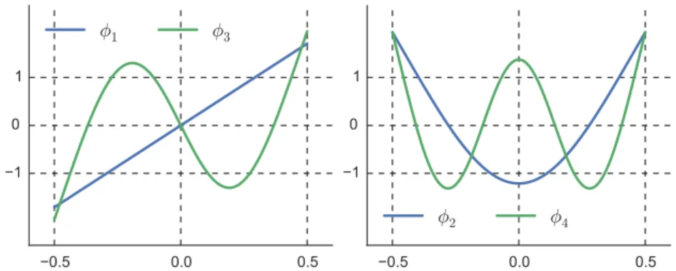
Figure 2.6.: Odd (left) and even (right) modes of the biharmonic operator with free boundary conditions at the sides.

Separation of variables is our best tools to construct a solution:

h(α, τ ) = X

n

χ

(τ )φ

(α) ,

where φ

are the eigenfunctions of the biharmonic operator ∂

for − 1/2 < α < 1/2:

φ

(α) = a

cos(q

α) + b

sin(q

α)

+ c

cosh(q

α) + d

sinh(q

α) , (2.26) with the eigenvalues q

and factors a

, b

, c

, d

that depend on the boundary conditions [66–68]. In the case of free ends, if the origin of the arclength is in the middles of the filament, the parity of the modes becomes evident:

φ

(α) =

cosh(ζ

α)

cosh(ζ

/2) + cos(ζ

α) cos(ζ

/2)

, n even φ

(α) =

sinh(ζ

α)

sinh(ζ

/2) + sin(ζ

α) sin(ζ

/2)

, n odd , (2.27)

where ζ

= (n − 1/2)/π and τ

=

π(n−1/2) L

. We plot the first 4 modes in Fig. 2.6.

Note that the Fourier modes are not a normal mode decomposition of Eq. (2.25).

This means that, on the contrary of the normal modes given in Eq. (2.27), each Fourier

mode will not display a single relaxation time. Nonetheless, the correct normal modes

2.4. Coupling Hydrodynamics and Elasticity

can be approximated by the Fourier ones when the wavelength is small compared to the filament length or the problem allows discarding the dynamics at the filament ends [69].

2.4. Coupling Hydrodynamics and Elasticity

We introduce here some theoretical background on the motion of a slender deformable filaments inside a viscous fluid. We have seen in Eq. (2.10) that the viscous drag is not evenly distributed along a filament, being stronger at the edges than at the center.

Classical slender body theory assumes the rod to be infinitely stiff and not deformable, hence the effective drag coefficients are obtained averaging the drag forces along the filament (Eq. (2.11)). This hypothesis is no longer valid when the body can deform, as it is in the case of semi-flexible filaments: the filament bends to comply to the uneven distribution of drag forces. The example of the elastic filament is a particular case of a more general behavior of deformable objects moving relative to a fluid (e.g.

in Ref. [70] the sedimentation of a red blood cell was studied): the viscous drag that develops on the body’s surface is not, in general, evenly distributed, hence objects deform to comply to the force; at the same time the new body shape generates new drag forces the body has to comply to; until a equilibrium configuration that balances drag forces and body forces is reached.

The dynamics of the position of a segment of the filament at position r(α, τ ) is determined by [67]:

∂

r(α, τ ) = Z

−1/2

dα

1

γ Iδ(r − r’)

D(α

)r’ + f ’ + Z

−1/2

dα

H(r, r’)

D(α

)r’ + f ’

(2.28)

where f is the external force density, γ = 3πη is the friction per unit length, D is the

biharmonic operator D = − ∂

that accounts for the bending energy, and H(r, r’)

is the Oseen tensor [67, 71]. Eq. (2.28) has been written to enhance the similarity

between its terms, but it can be split into its elementary contributions. Let us begin

by noticing that each integral is the sum of two contributions: a term proportional

to the external field f, that is equivalent to Eq. (2.9), and a term proportional to the bending rigidity ∂

r. Each term, in turn, can be seen as a contribution of a local term (first line) and a non-local term (second line).

Comparing Eq. (2.18) and Eq. (2.28) we recognize that the r.h.s. of the first line describes the elastic and external forces acting directly on position r. The second line couples the local dynamics with the fluid flow generated in points far from r.

The tensor H(r, r’) is the Oseen tensor:

H(r, r’) = Θ( | R | − b) 8πη k R k

IR

+ RR

(2.29) where Θ(x) is the Heaviside function, b is the filament radius and R = r − r’. With this formulation, the cutoff length is implemented directly in the definition of the tensor.

Decomposing the position r on the modes of the biharmonic operator as done for Eq. (2.25) the equation of motion for the modes is

∂

χ

= X

l

(H

+ δ

)

− χ

γ τ

+ f

(2.30) where Dφ

= − 1/τ

φ

and H

is the interaction matrix:

H

= Z

−1/2

dαdα

φ

(α)H(r, r

)φ

(α

) .

In the absence of hydrodynamic interactions, the modes do not mix and each mode relaxes with a unique relaxation time τ

. Eq. (2.30) shows that the hydrodynamic matrix H

mixes the modes and their relaxation times. When the external force f is uniform (as is the case of gravity), the force couples only to the zero-th mode because f

= 0 – the coupling between higher modes and the external force is due to the hydrodynamic matrix. Since the 0 − th mode is the center of mass position, in the absence of long-range hydrodynamics, the filament simply translates along the gravitational field and the other modes relax with their unaltered characteristic time.

In presence of hydrodynamics, instead, the filament bends upward [72] because the

2.5. Active Axonemes

+ f(s ) Δ

-f(s )

Molecular motor Semi- fl exible fi lament r

Base Center line

Shear force Displacement

Body

- -

+ Polarization

Polarization

Figure 2.7.: Sketch of the 2D axoneme. The sliding filaments (red) are like two rails, at fixed distance r. The molecular motors are attached at one side, and pull the opposite filament towards the + sign. The base (yellow) hinders the sliding, and connects the filaments to the sperm body.

hydrodynamic matrix couples the external uniform field to the higher modes that are, thus, excited.

2.5. Active Axonemes

The 9+2 structure of the axoneme hosts dynein motors between adjacent double- microtubules (Fig. 1.4, Fig. 2.4, and Fig. 2.7). Since the beating amplitude does not decrease, energy has to be provided throughout the flagellum length [37, 73]. It was soon realized that the sliding forces generated between the microtubules can indeed bend the filament and generate a traveling wave [37–39].

The question is, then, about the feedback mechanism between the filaments and

the molecular motors. In the very first model a simple curvature-feedback between

the viscous and elastic torques, and the active torques is proposed to model the

beating pattern of sea urchin (see Refs. [30, 31, 37–39, 74, 75]). In the most recent

developments the attention is turned to the actual mechanics that may generate the