Sperm and Cilia Dynamics

I n a u g u r a l - D i s s e r t a t i o n zur

Erlangung des Doktorgrades

der Mathematisch-Naturwissenschaftlichen Fakult¨at der Universit¨at zu K¨oln

vorgelegt von Jens Elgeti aus Bremen

K¨oln

2006

Tag der letzten m¨ undlichen Pr¨ ufung: 26.02.07

1 Introduction 9

1.1 Motivation . . . . 9

1.2 Axoneme . . . . 10

1.3 Sperm . . . . 14

1.4 Cilia . . . . 18

1.5 Theory . . . . 22

1.5.1 The Beating Axoneme . . . . 22

1.5.2 Sperm Motility . . . . 23

1.5.3 Cilia Dynamics . . . . 24

2 Method 27 2.1 Molecular Dynamics . . . . 27

2.2 Mesoscopic Hydrodynamics . . . . 28

2.2.1 Navier-Stokes equation . . . . 28

2.2.2 Low Reynolds-Number Hydrodynamics . . . . 29

2.2.3 Multi Particle Collision Dynamics . . . . 31

2.2.4 Units . . . . 34

2.2.5 Thermostat . . . . 34

2.2.6 Poiseuille Flow . . . . 35

2.2.7 Partially Driven Flow . . . . 37

2.2.8 Dimensionless Efficiency . . . . 38

2.2.9 Rod Friction . . . . 39

2.3 Sperm Model . . . . 42

2.3.1 Sperm Structure . . . . 42

2.3.2 Importance of Asymmetry . . . . 45

2.3.3 Sperm Simulations without Hydrodynamics . . . . 46

2.3.4 Rocket Model . . . . 48

2.4 Cilium . . . . 48

2.4.1 Cilia Structure . . . . 48

2.4.2 Control Parameters for Cilia . . . . 51

2.5 Boundary Conditions . . . . 52

3 Sperm Results 55 3.1 Important Observables . . . . 55

3.2 Free Movement . . . . 56

3.2.1 Simulations with Hydrodynamics . . . . 56

3.2.2 Simulations without Hydrodynamics . . . . 62

3.2.3 Discussion . . . . 67

3.3 Confined Movement . . . . 67

3.3.1 General Observations . . . . 68

3.3.2 Surface Adhesion . . . . 69

3.3.3 Regimes of Motion . . . . 76

3.3.4 Velocity in Thin Films . . . . 81

4 Cilia Results 83 4.1 How to Characterize Metachronal Waves . . . . 83

4.2 Extraction of Metachronal Wave Effects . . . . 88

4.3 Beat Period . . . . 88

4.4 Auto-Correlation Function . . . . 91

4.5 Wavelength . . . . 93

4.6 Orientation of the Metachronal Wave . . . . 93

4.7 Correlation Anisotropy . . . . 94

4.8 Correlation Lengths . . . . 95

4.9 Transport . . . . 97

4.10 Orientation of Transport . . . . 101

4.11 Energy and Efficiency . . . . 103

4.12 Planar Beating . . . . 107

4.13 Finite-Size Effects . . . . 107

4.14 Discussion . . . . 109

5 Conclusion and Outlook 111

6 Acknowledgments 115

7 Appendix 117

7.1 Parallelization . . . . 117

Sperm cells are propelled in a fluid by an active, snake-like motion of their tail, the flagellum. It is known for some time that sperm cells accumulate at the walls of a container, swimming mostly in clockwise circles. Cilia are hair- like extensions of some cells that propel fluid over its surface by performing a whip-like motion. Cilia appear in many places in nature, e.g. to remove mucus out from the human respiratory system, or on the surface of swimming Paramecium . One of the puzzling phenomena observed in large arrays of cilia, is the metachronal wave; neighboring cilia beat with a certain phase difference that leads to wave-like patterns, similar to those observed when the wind blows over a wheat field. Both structures, the flagellum and the cilium, have a very similar underlying structure, the axoneme. This similarity suggests a combined theoretical study.

We constructed a model axoneme that is used for simulations of sperm and cilia. It is modeled as a semi-flexible polymer, on which an active bending can be imposed. Hydrodynamic interactions, which are responsible for the directed motion of the cell and the metachronal wave of cilia, are taken into account by a particle-based, mesoscopic simulation technique (multi-particle collision dynamics). In sperm simulations, the axoneme is subjected to a sinusoidal bending force. The sperm head is modeled as a sphere, chirally displaced from the beat plane of the tail. Arrays of cilia are modeled by attaching several axoneme models to a wall. The activity is imposed by a geometry-dependent bending force.

We demonstrate that the highly simplified sperm model captures the main fea-

tures of cell motion described above. We unveil how hydrodynamic interactions

lead to adhesion to a wall, and we are able to explain this apparent attraction by

a combination of thrust and hydrodynamic repulsion of the tail. Furthermore,

we find that the chirality is the cause of the directed circular motion. Tuning

this chirality, we find two regimes of motion. In one regime sperm swim in tight

circles very close to the wall. Without rotation around the longitudinal axis of

the sperm cell, the beating plane stays perpendicular to the wall. In the other regime, the sperm follows large circles and rotates around its own longitudinal axis. In this case the beating plane is on average parallel to the wall. We explain the transition between these two regimes of motion by a dynamic change of the shape of the flagellum.

For cilia, we present, for the first time, a two-dimensional array of autonomously beating cilia, solely coupled by hydrodynamic interactions, that develop a metachronal wave. We show that the metachronal wave enhances velocity and efficiency of solute transport compared to synchronously beating cilia. The transport ve- locity increases up to a factor of 3.2, when the cilia are packed more densely, while transport efficiency increases almost an order of magnitude. Furthermore, we characterize transport and wave properties as functions of the viscosity, ef- fective stroke direction and cilia spacing. For example, we show that the main correlation direction roughly coincides with the effective stroke direction, and that the beat frequency decreases through metachronal coordination while the energy consumption per beat is largely independent of cilia spacing, effective stroke direction, and metachronal coordination. We believe, that for the fitness of the cell, both the efficiency and especially the transport velocity are essential.

The metachronal wave pattern is thus of great functional significance for ciliated

cells.

1.1 Motivation

Life, as we see it, is deeply connected to motion. Motion is commonly consid- ered to be a “sign of life”. Movement is important from single cells, to higher organisms. There are many kinds of cell motility:

Cell crawling, for example, is used by fibroblasts to move across a surface to repair a wound. White blood cells adhere to the wall of the blood vessel and crawl through tissue to combat an infection. Amoebae crawl across surfaces in their search for food. Typical velocities of crawling cells are on the order of 10 µm/s. The basic mechanisms of cell crawling are known [2]. First, the cell pushes filopodia, finger-like extensions, in the foreword direction. These filopodia adhere to the surface via adhesion molecules (integrin for example).

Thereafter, the cell body is dragged across the surface. How exactly these indi- vidual steps are performed, however is subject of ongoing research (see Ref. [72]

for a review).

Some bacteria use rotating flagella to swim through a fluid to find food; Es- cherichia coli is probably the best-known example. This rod-like bacterium has a bunch of roughly 20 µm long helical threads connected to motor proteins. When the threads rotate counterclockwise, they form a bundle and act as a propeller that moves the bacterium foreward. On the other hand, when the rotation of the flagella is clockwise, E.coli starts to tumble and to reorientate. The motor creating the necessary torque [84, 80] and the formation of bundles [70, 48] were examined in recent years.

The bacterial flagella should not be mistaken with the eukaryotic flagella de- scribed below. In this work the term flagellum always refers to the eukaryotic flagellum.

Sperm use a beating flagellum to swim towards the egg. Paramecium, a uni-

cellular organism, is covered by thousands of beating cilia to propel it through a

fluid. Both, cilia and flagella, are built from an axoneme, which is a very univer-

sal structure throughout the animal kingdom. Sperm tails, propelling hairs on a Paramecium, small hairs in the respiratory system and many other examples are all constructed essentially in the same way. Furthermore, flagella are of interest for engineering [50] e.g. for micro machines [18]. For example, Dreyfus et al.

[18] constructed a chain of magnetic colloids that are moved by an external field in a sinusoidal pattern, and thus create thrust on an attached red blood cell.

The common axoneme structure, its wide appearance in eukaryotic cells, and its potential for engineering makes the understanding the dynamics of cilia and flagella, the hydrodynamics around them, the propulsive forces and collective phenomena a field of research of fundamental interest. We develop a coarse- grained model with only a few parameters. Using computer simulations, we are able to reproduce and study large-scale phenomena of motility. This will be the theme of this work.

1.2 Axoneme

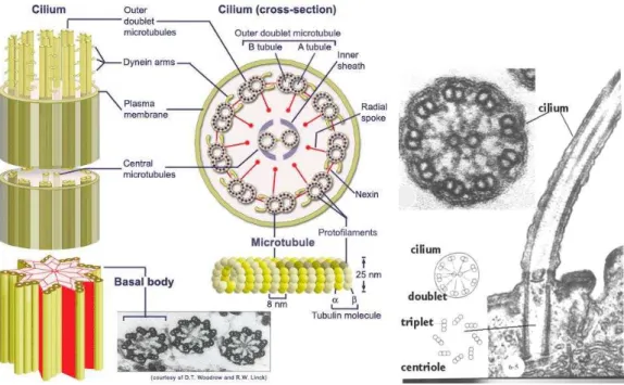
The structure underlying cilia and flagella is called the axoneme. The axoneme is constructed from approximately 250 different proteins [42]. Small differences occur between the axonemes of different organisms, but the basic design is the same, which is the ”9+2 Structure”. Two central microtubules (stiff polymers, the “bones” of the cytoskeleton) are surrounded by 9 double microtubules (see Fig. 1.1). These microtubules are connected by many proteins to create the ap- propriate elastic properties. At one end, the doublet microtubules emerge from a basal body (see Fig. 1.1) where they form triplets with another microtubule.

Motor proteins (dyneins) cause an active bending of the structure by sliding microtubules along each other. The generation of motion is illustrated in Fig.

1.2.

It is not yet fully understood how these motor proteins are controlled. Several models have been proposed (see Sec. 1.5). The “9+2 structure” is enclosed by an extension of the cell membrane, in contrast to bacterial flagella which are bare protein threads extending from the cell.

In the following, the key components of the axoneme are described in more detail.

• Microtubules are long and stiff polymers that are found in several other

structural units of a cell. Together with other protein filaments, they form

Figure 1.1: Structure of the axoneme Left: Schematic figure of the axoneme, from

http://www.nyu.edu/classes/ytchang/book/e003.html Right: Micrographs of a cilium, from

http://www.cytochemistry.net/Cell-biology/cilia_intro.htm

Figure 1.2: Microtubule sliding leads to bending . On the left side is a relaxed two dimensional model of the axoneme, in black the two microtubules and in red the motor proteins. The green arrows indicate that the motor proteins will move along the left microtubule upwards about 10% of their current distance from the base. Because the microtubule is attached at the lower end, it is bend as pictured on the right hand side.

the cytoskeleton of the cell. They consist of tubulin monomers that are ar- ranged in a helical fashion to form a hollow tube (see Fig. 1.3). These tubes are about 24 nm thick and can be up to millimeters long. Microtubules are rather stiff with a persistence length of several millimeters. Inside a cell, microtubules may be dynamically unstable, constantly polymerizing and depolymerizing. This dynamic instability is used, for example, to form the meiotic spindle [13, 28]. In the axoneme, special proteins keep the microtubules from falling apart. The outer ring of microtubules in the axoneme is formed by doublet microtubules, always two microtubules are interlaced into each other. In a cross section view, doublet microtubules look like three quarters of a circle that is attached to the full circle of a normal microtubule (see the micrograph in Fig. 1.3).

• Dyneins are motor proteins that use ATP hydrolysis to move along a

microtubule. They are the key active component of the axoneme. More

precisely: cilia and flagella have so-called axonemal dyneins that have two

different arms extending clockwise from one doublet microtubule to the

next.

Figure 1.3: Microtubule structure.

Left: 3-D reconstruction of a microtubule from http://en.wikipedia.org/wiki/Microtubule

Right: An electron micrograph of a cross section of a cilium, from http://www.cytochemistry.net/Cell-biology/cilia_intro.htm

In a cell, a large variety of motor proteins is present to fulfill many different tasks. Motor proteins have been studied intensively in recent years. In a typical experiment, a colloidal particle is attached to one end of the motor protein. In an appropriate solution, the motor proteins run along a microtubule, while a laser tweezer can exert a well-defined force onto the colloid. Thus a velocity versus force measurement is possible [21]. Motor proteins have been described as “Brownian ratchets” [73]. In a spatially periodic yet asymmetric potential, which switches periodically directed motion is possible - even against a net force.

• Radial spokes form a class of proteins (about 22 have been identified) that connect the central pair with the outer ring. It is speculated that some of these radial spokes act as regulators for the inner dynein arms [42], but their precise function is still unresolved.

• Membranes can self assemble from a solution of amphiphilic molecules.

A simple artificial membrane is a lipid bilayer that forms in an aqueous

solution by the hydrophobic effect. In cells, membranes are much more

complex. Many different kinds of lipids, proteins, glycolipids, cholesterol

and other ingredients are embedded into the membrane. A schematic

view is shown in Fig. 1.4. In the cell, the main function of membranes is

Figure 1.4: Cell Membrane [5].

to provide a barrier between the cytoplasm (the interior of the cell) and the surrounding fluid, but it is also essential for many other processes [2], including ATP synthesis, transport (endocytosis, exocytosis) and adhesion.

The membrane seems not to be essential for axoneme dynamics and the generation of flow; Brokaw [7] showed that sperm can swim without a membrane.

• Many other proteins and structures can be found in the axoneme. Among others, there are nexin links, protein kinases, fibers, pores, ion channels, receptors etc. Their function varies from beat pattern control and sensory functions to elastic stiffening.

For a more detailed description of the structure of the axoneme, see Ref. [42].

1.3 Sperm

Sperm motility has been studied for a long time. Rothschild’s review [78] on the sea urchin spermatozoon in 1951 covered the first 27 pages of “Biological Review”, while a search for “sperm” in the Web of Science leads to over 50 000 hits. From a physics point of view, the motility of sperm is probably one of the most interesting topics of research. An essay by Brokaw [8] provides a lucid review of the history of sea urchin sperm motility, subtitled “My Favorite Cell”.

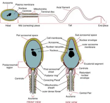
Although sperm cells from different species look different, they have a similar

structure from a theoretical point of view: A long flagellum is attached to a

relatively small head (see Fig. 1.5).

Figure 1.5: Diagram of human sperm, from http://en.wikipedia.org/wiki/Sperm

Many substructures are present in sperm (see Fig. 1.5). Starting from the tip of the head, called acrosome (used to “dig” into the egg) to the nucleus, where the haploid genetic information is stored, to the flagellum, where in the axoneme many mitochondria are wrapped around the “9+2 structure” to provide ATP as energy source. Chemotaxis, the directed motion in a chemical gradient, is accomplished by a combination of complicated sensory responses involving a cascade of protein-protein interactions. The flagellum is separated into (at least) three parts: the mid piece, the principal piece (which can be subdivided in further pieces), and the end piece.

It is instructive to take a look at the characteristic length scales of, for ex- ample, sea urchin sperm [26]. The head appears triangular or conical in shape, about 3 µm long and 1 µm thick. The flagellum is much larger; it has a length of roughly 50 µm. At the surface of the cover slip, the sperm swims with a di- ameter of 50 µm [46] (see Fig. 1.6) at a velocity of roughly 220 µm/s (although these values depend somewhat on the degree of activity).

Motion of sperm is created by beating of the tail. The beat pattern is, like

the overall structure, species-dependent, but on a more global level, the peat

patterns are similar [83, 6]. The beat pattern has the form of a traveling bend-

Figure 1.6: Sea urchin sperm, swimming at a surface (from Ref. [46], scale bar is 50 µm).

ing wave, usually from the head to the tip of the tail, but the reverse is also reported. This bending wave can be sinusoidal, but also half circles in opposing directions or meander-like beat patterns have been reported. Typically the flag- ellum beats essentially in a single plane, although some form of a small aplanar beat component is reported for many species while others might even display an almost helical beat pattern.

In bulk fluid, sperm usually swim on helical trajectories. In confined ge- ometries, like in the droplet between the cover slides under a microscope, sur- prisingly sperm accumulate at the walls. In 1963, Rothschild [79] observed this phenomenon quantitatively and concluded that some hydrodynamic interactions capture the sperm at the surface. This basic observation is not yet understood.

More recently the problem of sperm adhesion was addressed by Cosson et al.

[12] and Woolley [94]. Cosson et al. [12] studied sea urchin sperm using high- speed video microscopy. They observed that parts of the sperm tail close to the surface are out of focus. This was interpreted as an out-of-plane component in the beating pattern. It was further argued that this out-of-plane component generates a force that pushes the sperm towards the surface.

Woolley [94] distinguishes two different forms of surface adhesion of sperm

displaying either a planar or a three-dimensional beat pattern. For planar beat-

ing sperm, the key observation is the “left-hand rule”: sperm only adhere to a

surface if the left side of the head touches the wall. Woolley assumes that, due to asymmetries, the head acts as a hydrofoil and thereby creates a pressure against the surface in one direction. Sperm with a three-dimensional beat pattern on the other hand adhere if the beating envelope is conically shaped. If one side of the cone is close to the wall, the thrust points towards the surface, thus keeping the sperm at the surface.

Furthermore, once captured at the surface, sperm swim in a circle with a preferred direction of rotation. This circular motion is not just the projection of the helical bulk trajectory. Woolley [94] proposed that the preferred circling direction arises because only one side (“left”) of the head adheres to the surface.

In the case of a three-dimensional beating pattern Woolley argues that, while the sperm is rotating, the head experiences higher viscous friction close to the wall. Thus the resulting forces are turning the sperm in the same direction of its rotation (if observed from the front of the sperm’s head / from outside the observation chamber).

An important question that is beyond of the scope of this work is how chemo- taxis induces directed motion of sperm. The group of Kaupp [46, 35, 45, 85] has made significant progress by understanding how binding of a chemical attrac- tant released by the sea urchin egg, leads to changes in the sperm trajectory and thus to chemotaxis. While swimming in circles, the sperm senses the chemo- attractant concentration. A calcium influx causes an increase in the curvature of the trajectory after some time delay. Thereafter, the sperm swims straight for a while before swimming in circles again. With the correct match of the velocities and delay times, the sperm is able to swim up gradient, towards the egg.

Although many models that describe the beat pattern of the flagellum have

been developed (see Sec. 1.5), no consistent model explaining the different

dynamical phenomena on larger length scales has been proposed. In this thesis,

we provide a simple model, only considering some basic characteristics of a sperm

cell. We are able to reproduce sperm behavior in a qualitative form in bulk fluid

as well as in confined geometries. In particular we are able to explain how sperm

adhere to a wall due to hydrodynamic repulsion of their tail. Furthermore, our

model is flexible enough to implement specific beat patterns and geometries in

future studies.

1.4 Cilia

Cilia are active hair-like extensions from the cell that can, by performing a whip- like motion, move fluid across the cell surface. They are typically 5-20 µm long and about 250 - 1000 nm thick.

Probably cilia have already been discovered in 1675 [82] and described as little legs used for propulsion of a unicellular organism. Over the years, more and more details were discovered. Cilia appear in many different forms. For

cilia

Figure 1.7: Stentor ciliate, from wikipedia,

http://en.wikipedia.org/wiki/stentor%28genus%29

example Stentor (see Fig. 1.7) is a group of filter feeding ciliates named after the Greek herald Stentor due to their trumpet-shaped body. Around the “mouth”, a ring of cilia bundles moves fluid and nutrition inside the body. The Paramecium (“Pantoffeltierchen”) is one of the most famous unicellular eukaryotes. Cilia, on

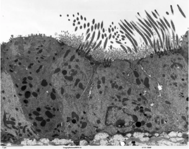
Figure 1.8: Transmission electron microscope image of the lung (mouse). From

http://remf.dartmouth.edu/images/mammalianLungTEM/source/12.html

the surface of Paramecium are used for propulsion of the cell through aqueous medium. In the female reproductive tract, the oviduct, large arrays of cilia move the egg. In the lungs of mammals (see Fig. 1.8), cilia propel mucus out of the respiratory system. All these different cilia have a remarkably similar structure, the axoneme. The differences are mainly in size and beating pattern (see Fig.

1.9). While the beat pattern of sperm is relatively symmetric, cilia have clearly distinguishable effective and recovery strokes. The relatively fast effective stroke (also called power stroke) happens in a plane perpendicular to the surface while the cilium is rather straight. In the recovery stroke, the cilium slowly returns back to the initial position, moving more closely at the surface in a plane tilted towards the surface. Due to the asymmetry of this beat pattern, fluid is moved in the effective stroke direction (ESD).

Effective Stroke 2

1 3

4

5 6 7 8

9 10 11

12

Figure 1.9: Cilium beat pattern, schematic drawing. The effective stroke (1-4) is much faster than the recovery stroke (5-12). Redrawn from [82].

Ciliated cells are often much larger than the cilia itself (see Fig. 1.8). Typi-

cally, cilia appear in large arrays. A single organism, like Paramecium , is covered

by thousands of cilia (see Fig. 1.11). Cilia do not beat randomly or uncoordi-

nated. Instead, they beat in a coordinated wave-like pattern which is called a

metachronal wave (see Fig. 1.10). The metachronal waves look similar to those

when wind blows offer a wheat field.

Figure 1.10: Metachronal waves of cilia in Opalina, from [86]. (a) Bar=100 µm,

(b) Bar=10 µm, (c) Bar=10 µm. Waves travel in the direction of

Figure 1.11: Paramecium covered with cilia, from http://www.biomedia.cellbiology.ubc.ca

The properties of the metachronal wave of the cilia depend strongly on the system. One distinguishes symplectic metachronism where the wave propagates in the direction of the effective stroke, antiplectic metachronism, where the wave travels in the opposite direction, and dexioplectic and laeoplectic metachronism, where it travels perpendicular to the effective stroke [82]. It is known that for certain cilia increased viscosity of the fluid decreases the beat frequency but can also cause erratic behavior [22].

As an example for metachronal waves, consider the work of Gheber et al.

[22, 23, 24]. The authors study a monolayer of tissue culture of frog esophagus

(the tube that leads from the frog’s mouth to the stomach) using optical fibers

to get simultaneous data from different points. These mucus propelling cilia are

5-7 µm long and about 600 nm thick. They beat with about 15 Hz and form a

metachronal wave traveling at 90-125

clockwise to the effective stroke direction

with a wavelength of 5-9 µm.

1.5 Theory

One of the earliest theoretical works on sperm motility is the article by Gray and Hancock (1955) on “The propulsion of sea-urchin spermatozoa” [27]. The propulsive speed of the whole sperm is calculated as a function of the shape and the speed of propagation of the bending waves that are generated by the tail (see Sec. 1.5.2). Several more complex theories have been developed later on. We will discuss a selection in theory of The Beating Axoneme (Sec. 1.5.1), Sperm Motility (Sec. 1.5.2), and Cilia Dynamics (Sec. 1.5.3).

1.5.1 The Beating Axoneme

In 1994, Lindemann introduced the “geometric clutch” hypothesis [56]. It has been developed further recently (see for example Ref. [58] and Lindemann’s review [57]). In this model, transverse forces, due to active or passive bending, move adjacent microtubules further apart or closer together. Because in this model the dynein activation probability depends on the distance between the microtubules, a geometrical feedback from the configuration of the axoneme to the active bending force is achieved. Hence the name “geometric clutch”. By adjusting the mechanical properties of the model, different cilia and flagella can be simulated. After further adjustment the model reproduced experiments in which the outer dynein arms were removed, and even predicted two types of arrest behavior that were subsequently experimentally verified.

Brokaw [11] developed a curvature-controlled mechanism for the axoneme.

Dyneins are modeled as groups which are switched off whenever the local cur- vature exceeds a certain preset value. Thereafter, the group on the opposite side is activated. In a series of studies, he was able to describe many different phenomena such as sinusoidal beat patterns of arrest behavior [9, 10, 11]. Both Lindemann [58] and Brokaw [11] implemented hydrodynamics only at the level of an anisotropic friction (see Sec. 1.5.2).

Dillon et al. [16] simulated a two-dimensional axoneme with the immersed boundary method for hydrodynamics. The authors simulated the axoneme as an elastic structure, and dyneins as springs within. The dynein activation is also curvature controlled. The authors do not attempt to reproduce the exact beat pattern of cilia from a specific organism, but define parameter ranges in which beat patterns of both, cilia and flagella, are observed.

The immersed boundary method was introduced by Peskin [68] to model blood

flow in the heart. Here the Navier-Stokes equations are solved numerically on a grid, boundaries are taken into account by δ-function forces. The main idea is that the object is modeled by a volume of fluid, and its movement is produced by forces on its surface (see Ref. [69] for details).

J¨ ulicher and Prost [44] showed that competing forces produced by motor pro- teins lead to instability and oscillations. Hilfinger and J¨ ulicher [36] used this ability of a collection of molecular motors to exhibit spontaneous oscillations [44] and rigorously calculated the dynamics of an actively bending rod [36].

These studies provide a detailed and impressive comparison between theory and experiments on sperm.

To conclude, the overall beat pattern is well reproduced by different models, whereas the details of the beating strongly depend on the individual features of the axoneme. Often the models are able to describe many different beat patterns of different cilia or flagella by small changes in a few parameters.

1.5.2 Sperm Motility

Gray and Hancock [27] calculated the swimming velocity of sperm cells. Using the fact that the two friction coefficients for a rod dragged parallel (γ

) or perpen- dicular (γ

) to its orientation are different, they calculated the force generated by a moving element of the tail. After assuming a sine-shaped beat-pattern, γ

= 2γ

, and some other approximations, they calculated the swimming speed as,

¯

v

= ωπb

λ 1 + 4π

b

λ

−

r

1 + 2π

b

λ

C

nλγ

!

(1.1) where ω is the angular frequency, λ the wavelength and b the amplitude of the beat. The number of waves present on the tail is denoted by n, C

is the drag coefficient of the head. For a spherical head of radius a and a thin tail of radius d, it is possible to approximate

C

γ

= 3a

log d

2λ

+ 1 2

. (1.2)

Because a pre-defined beat shape has been used, the viscosity η does not influ- ence the swimming speed.

Fauci and McDonald [20] simulated a two-dimensional sperm in thin films with

the immersed boundary method. They conclude that the sperm’s swimming

speed is inversely proportional to the width of the film d,

¯

v

= 1 A

+ B (1.3)

where b is the beat amplitude and A and B are constants. They also observe an effective attraction to the wall. The results strongly depend on the dimension- ality. In three dimensions, the fluid can flow around a slender filament, whereas in two dimensions it is confined to one side.

1.5.3 Cilia Dynamics

Netz and coworkers [49, 62] studied a cilia-related model in form of an elastic rod. In the study by Netz and Manghi [62], the rod is grafted to a rotary motor.

Due to the hydrodynamic drag the rod bends and thus creates a flow away from the plane to which it is attached.

The study by Kim and Netz [49] is more closely related to cilia. The rods are attached to an angular motor. During the effective stroke, a rather weak torque forces the rod to move in one direction while its shape is essentially a straight rod. The high torque during the recovery stroke bends the rod, and thus less fluid is transported than during the effective stroke. This is in contrast to the biological situation, but it might be helpful for engineering of micropumps.

Kim and Netz [49] define a dimensionless efficiency

ǫ = (D/a)/(E/k

T ) = (¯ v/a)/(∂

E/k

T ) (1.4) where D and E are the pumping distance and energy per beat cycle, respectively, and a is the rod diameter. They find a line of highest efficiency in the persistence- length versus torque parameter space.

J¨ ulicher and Vilfan [91] presented a model where a cilium is represented by a single sphere on a tilted elliptical path near a planar surface. The sphere is driven by a predefined tangential force while hydrodynamic interactions are taken into account by Oseen tensor calculations. Because wall friction reduces the amount of pumped fluid when the sphere is closer to the wall, a net fluid flow results. Modeling two cilia, they were able to identify areas in parameter space where synchronization occurs and calculate the phase lag explicitly.

Lagomarsino, Jona and Bassetti [51] simplified the cilium to a rower. A rower

can be considered as a point particle with a power and recovery stroke. In the

effective stroke, its hydrodynamic drag coefficient is increased and the potential

is switched to move the particle in another direction compared to the recovery stroke. This way the rowers can generate a net flow. A geometric feedback is achieved by switching between the two strokes when a certain displacement is reached. Hydrodynamic interactions are modeled by the Oseen tensor, but no walls are taken into account. The hydrodynamic interactions and the geometric feedback together allow a coupling and synchronization of the rowers. In the continuum limit, in which the model can be studied analytically, the authors only find a stable metachronal wave if the hydrodynamic interaction is negative (i.e.

hydrodynamic forces are attractive). But in simulations they find also short- wavelength traveling wave packets where neighbors beat in an anti-correlated fashion.

Gueron and Levit-Gurevich [32, 33, 31, 30] modeled the cilium as a slender, elastic filament. Switching between effective and recovery strokes is defined by the curvature of the cilium. Hydrodynamic interactions are taken into account by a slender body theory [34], which in turn incorporates hydrodynamics with a Oseen tensor approximation. In two dimensional studies [30], where all move- ment is restricted to one plane, they find an antiplectic metachronal wave; the beat frequency decreases with increasing viscosity and distance between cilia.

Furthermore they calculated the energy expenditure per effective stroke to be 9 · 10

J which decreases to 3 · 10

J for 100 densely packed cilia in a row.

During the recovery stroke the energy expenditure is 2 · 10

J [31], indepen- dent of the number of cilia. The three-dimensional model also includes effects of ATP concentration [32], but the cilium is not allowed to twist. Simulations of 5 × 5 cilia arrays show a metachronal pattern, but a detailed analysis of the metachronal wave was not presented. In the most recent model [33], a twist of the cilium is introduced and singularities in the equations of motion are removed.

This model has not yet been used to study cilia dynamics systematically.

Our goal is to find a rather universal model to simulate the large scale dynamics of flagella and cilia. The beat pattern is treated as an input parameter, and we study the large scale dynamics resulting from it. We do not simulate flagellar beating on a molecular level, but prefer a coarse grained description. Therefore, we treat the axoneme as an active crane-like polymer and the fluid around it with the mesoscale simulation technique MPCD. Details, like the beat pattern, axoneme length, boundary interaction, etc. can be subsequently adjusted to the specific system or model.

2.1 Molecular Dynamics

In a coarse-grained description, a group of atoms is represented by a bead or monomer, a point particle with a certain mass and well defined interactions. The movement of this particle is treated classically, i.e. it follows Newton’s equations of motion,

m

d

dt

~r

= F ~

. (2.1)

where m

, ~r

and F ~

are the mass, position, and force of monomer i respectively, and t denotes the time. In molecular dynamics, these equations are solved in discrete time steps. The straightforward discretization (known as the Euler algorithm) is known to be inefficient. Very small time steps are needed to get reasonably accurate results. Many algorithms have been proposed with different success. Here we use the well established Velocity Verlet Algorithm. Velocities and particle positions are updated according to the rule (see for example Ref.

[4]):

~r

(t + ∆t) = ~r

(t) + ~v

(t)∆t + ∆t

2m

F ~

(t) (2.2)

~v

(t + ∆t) = ~v

(t) +

F ~

(t) + F ~

(t + ∆t) ∆t 2m

. (2.3)

This algorithm has proven to be rather stable and efficient. Its main advantage is the time reversal symmetry and accuracy of O(∆t

). The time step ∆t has to be sufficiently small to guarantee energy conservation. In our simulation, energy conservation is not so critical, because we couple the system to a heat bath thus long term energy stability is not as critical. The time step ∆t must be small enough to allow correct integration of Newton’s equations. We used

∆t = 0.001 in most simulations presented here, and used the energy fluctuations of the molecular dynamics to ascertain that the time step is sufficiently small.

2.2 Mesoscopic Hydrodynamics

Hydrodynamic interactions are forces mediated by a surrounding fluid (or gas, then also called aerodynamics). In principle they arise from the movements of fluid particles and their interactions. We encounter them frequently in every day life. Whether it is wind slowing down a cyclist, pumping of the heart, water sprinkling from the garden hose or birds flying in the air, its all hydrodynam- ics. In many biological systems hydrodynamics play an important rule, and is essential in this work.

2.2.1 Navier-Stokes equation

The macroscopic hydrodynamics have been intensively studied on the basis of the Navier-Stokes equation

[54]:

ρ ∂~v

∂t + ρ(~v ~ ∇ )~v = η ∇

~v − ∇ p + f ~

(2.4) where ρ and ~v are the fluid density and velocity field. p is the pressure and f ~

is the external force density. The Navier-Stokes equation is derived explicitly from the standard Newtonian equations of motion, assuming that different “fluid particles” moving beside each other experience friction depending on the velocity gradient and the viscosity η (the “friction coefficient” of the fluid). Together with the continuity equation these equations fully determine the flow of an isothermal incompressible fluid. Thermal fluctuations however are not included.

1

for incompressible flow and without thermal fluctuations

By rescaling with a typical length scale l and velocity scale u, t

= tv/l

v

= v/u x

= x/l

p

= lp

ηu f

= l

f

ηu

the Navier-Stokes equation can be rewritten to a dimensionless form.

Re ∂~v

∂t + (~v ~ ∇ )~v

= ∇

~v − ∇ p + f ~

(2.5) The primes

have been omitted for simplicity. The dimensionless Reynolds number

Re = ρul

η (2.6)

describes the ratio between viscous and inertia forces. It is an important param- eter to characterize the type of flow; if the boundary conditions and the Reynolds number are the same, the flows are similar. The higher the Reynolds number, the more important are the kinetic, nonlinear terms, therefore the transition to turbulence is characterized by a system-specific Reynolds number.

Solving the Navier-Stokes equation for complex fluids and biological systems can be nearly impossible because of the complications that arise from coupling the Navier-Stokes equation to the immersed particles and complex boundary conditions. Thus other approaches are needed.

2.2.2 Low Reynolds-Number Hydrodynamics

In typical mesoscale systems, length scales are in the order of micrometers, velocities in the order of a few hundred µm per second. With the viscosity of water of 0.001 kg/ms, the Reynolds number is in the order of 10

. Thus the kinetic term

∂~v

∂t

+ (~v ~ ∇ )~v

in eq.(2.4) can be omitted, which simplifies the Navier-Stokes equation to the Stokes equation (or creeping flow equation):

∇ ~ p − η ∇

~v = f ~

(2.7)

Because the equation is now linear, solutions can be superimposed. The Oseen

tensor T and the pressure vector ~g are the Green’s functions for the creeping flow

equation (2.7). If the Oseen tensor is known, the velocity field can be calculated via

~v(~r) = Z

T (~r − ~ r

) f ~

( r ~

)d~ r

(2.8) and the pressure via,

p(r) = Z

~g(~r − r ~

) · f ~

( ~ r

)d~ r

. (2.9) For the bulk fluid, and for a single wall, the Oseen tensor is known. The explicit expression for the bulk fluid Oseen tensor [15]

T (~r) = 1 8πη

1 r

1 + ~r ⊗ ~r r

(2.10) shows the long range 1/r dependence of hydrodynamic interactions. (Here ⊗ represents the dyadic product, the result is therefore a tensor with the com- ponents (~r ⊗ ~r)

= r

r

.) Thermal fluctuations can be included for Brownian dynamics simulations [64], but require the inversion of the Oseen tensor to sat- isfy the fluctuation-dissipation relation. This approach is widely used in many mesoscale hydrodynamic simulations.

But also Oseen tensor calculations have their disadvantages. The main disad- vantage is that, computation times due to the matrix inversion are of the order N

(where N is the number of beads) which limits Brownian dynamics simu- lations with Oseen tensor hydrodynamics to date to a few hundred particles.

Because we want to model large arrays of cilia, and probably several interacting sperm, we used a more suited algorithm presented below.

In order to overcome such problems, many mesoscopic simulation techniques have been developed. Here a distinction can be made between lattice methods (e.g. Lattice Boltzman [63, 52]) and continuum methods (dissipative particle dynamics (DPD) [37, 19, 29], MPCD (as introduced below) and others, see Ref.

[74] for an instructive description). Without going into detail of the advantages and disadvantages of all these methods, we will explain our method of choice, multi particle collision dynamics (MPCD). Its main advantages are explicit local energy and momentum conservation, straightforward coupling to immersed ob- jects, easy implementation of complex boundary conditions and computational efficiency.

On the other end of the description of complex systems are atomistic simula-

tions with explicit solvent. However, due to the size of micro biological systems,

typically several µm, the number of particles (10

− 10

) makes this impossible.

Atomistic simulations can be a good option for smaller length scales.

2.2.3 Multi Particle Collision Dynamics

Multi-particle collision dynamics (MPCD) was introduced by Malevanets and Kapral in 1999 [60]. MPCD is a particle-based off-lattice method to simulate a hydrodynamic solvent.

The fluid is represented by a number n of point particles with positions r

and velocities v

that vary continously in phase space. The dynamics of these particles evolve in two steps:

• The streaming step, in which particles propagate freely according to their velocities for a collision time step h

~r

(t + h) = ~r

(t) + h~v

(t). (2.11)

• The collision step, where the particles are sorted into boxes and their relative velocities to the center of mass are rotated in a random direction by a preset angle,

~v

(t + h) = ~v

(t) + R (~v

(t) − ~v

(t)), (2.12) where R is the random rotation matrix and v

is the center of mass velocity of the box containing particle i. The box lattice constant is called a.

The random rotation matrix rotates a vector by a constant angle α around a random direction. This direction can either be chosen randomly from one of the six coordinate axes (this work) or form the surface of the unit sphere. Both lead to very similar transport coefficients [90]. Ripoll, Mussawisade, Winkler and Gompper [75, 76] showed that α ≈ 130

in combination with a small time step h leads to high Schmidt numbers (the ratio between viscous and diffusive momentum transport), i.e. fluid-like behavior. Thus we chose α = 130

in all our MPCD simulations.

From the algorithm, we see that energy and momentum are conserved. The

streaming step obviously does not change either momentum or energy. The same

can be shown for the collision step by a short calculation. For the momentum in each box:

P ~ (t + h) = X

iin box

m

~v

(t + h) (2.13)

= X

iin box

m

h ~v

(t) + R (~v

(t) − ~v

(t)) i

(2.14)

= X

iin box

m

~v

(t) + R X

iin box

m

(~v

(t) − ~v

(t))

| {z }

=0

(2.15)

= P ~ (t) (2.16)

Similary, we can deduce the energy E conservation:

E(t + h) = X

iin box

m

2 v

(t + h) (2.17)

= X

iin box

m

2 (v

(t) + R (v

(t) − v

(t)))

(2.18) (2.19) using the orthogonality of R

E(t + h) = X

iin box

m

2 v

(t)

(2.20)

= E(t) (2.21)

The collision step, being on a lattice, breaks Galilean invariance. Translational symmetry is via the Noether theorem connected to Galilean invariance, but the lattice breaks this symmetry. Another way to phrase this is that two particles, being in the same box in one frame of reference, are in a different box in a different frame of reference. To restore symmetry, and thus Galilean invariance, Ihle and Kroll [39] introduced a “random shift” - a displacement of the grid of collision boxes by a random vector where each component is chosen from the interval [0, a). Thus for the two particles to be in different boxes due to motion relative to the lattice just resembles a different result in drawing the random vector. Ihle and Kroll proved in Ref. [40] that this addition restores Galilean invariance to the MPCD algorithm.

For the implementation of walls, i.e. no-slip boundary conditions, particles

are bounced back, i.e. their velocity is inverted when they hit a wall. However

this procedure is not sufficient to create no-slip boundary conditions [53]. The wall has to be considered in the collision step as well. If the wall cuts a box in half, only half as many particles are inside the box on average. During the collision step, these particles should somehow collide with some of the particles of the wall. This can be done in the following way:

If during the collision step boundary cells are only partially filled (i.e. the number of particles in the cell ρ(i) is less than the average number of particles ρ in the cell), virtual particles are added. Because the wall particles should have a finite temperature, these virtual particles have Gaussian distributed velocities (i.e. energies distributed according to a Maxwell-Boltzmann distribution) and are generated independently for each step. Because the sum of Gaussians is again a Gaussian distribution this can be simplified by adding a random vector whose components are drawn from a Gaussian distribution of zero average and variance (ρ(i) − ρ)k

T . This scheme, introduced by Lamura, Gompper, Ihle and Kroll [53], has proven to provide nearly perfect no-slip walls.

The viscosity can be calculated analytically with a molecular-chaos assump- tion [47, 41, 90],

η = η

+ η

(2.22)

η

= m(1 − cos α)

18ha (ρ − 1) (2.23)

η

= k

T hρ a

5ρ

(4 − 2 cos(α) − 2 cos(2α))(ρ − 1) − 1 2

, (2.24)

where η

is the collisional, and η

the kinetic contribution to the total viscos- ity. These analytic expressions allow to test the implementation of the algorithm.

Besides checking the obvious conservation of energy and momentum, the viscos- ity can be measured. We perform this test in the Poiseuille flow (see Sec. 2.2.6).

For a more detailed description of the method see e.g. Refs. [93, 76].

Coupling of the fluid to polymers or other immersed particles is straightfor- ward. Polymers, modeled on a coarse-grained level by monomer beads connected by harmonic springs, are simulated by standard molecular dynamics described above. The polymers can be coupled readily to the MPCD fluid by including the monomers in the collision step [61]. This has been shown [93, 76] to reproduce the hydrodynamic behavior of polymers as described by Zimm dynamics.

Furthermore, with MPCD hydrodynamics can be turned off and on easily.

This is useful to extract the effects of hydrodynamics in a given system. Sim-

ulations without hydrodynamics are performed by assigning each monomer an

individual collision box. Within each of these collision boxes are ρ particles with Gaussian distributed velocities similar to the virtual particles used for no- slip walls. The collision step and the molecular dynamics for the monomers are not altered. With this scheme, hydrodynamic interactions are not present, but the thermodynamic properties are the similar. Thus, we are able to simulate the same systems with and without hydrodynamics.

Because its introduction in 1999 [60], MPCD has been successfully applied to study different physical systems. Ripoll, Winkler and Gompper examined the behavior of star polymers in shear flow [77], and together with Mussawisade they studied rod-like colloids in shear flow [92]. Noguchi and Gompper used MPCD to investigate vesicles in shear flow [65] and red blood cells in capillary flows [66]. Ali, Marenduzzo and Yeomans applied MPCD to the packing of polymers in viral capsids [3]. To analyze the influence of hydrodynamics on sedimentation of colloids, Padding and Louis [67] also used MPCD. Tucci and Kapral expanded the method to study reaction-diffusion fronts [88]. The group of Ohashi extended MPCD to multiphase fluids [43] and ternary amphiphilic fluids [81]. To describe a fluid with a non-ideal equation of state, MPCD was expanded by T¨ uzel, Ihle, and Kroll [89].

2.2.4 Units

For convenience, we rescaled time and distances to dimensionless units via x

= x/a and t

= t p

k

T /ma

. This is equivalent to choosing a = 1, k

T = 1, m = 1, resulting in the mean free path λ

= h p

k

T /m = h. All simulation results will be given in these dimensionless units.

The dynamic regimes of the MPCD fluid depends on the input parameters, especially the rotation angle α, the particle density ρ and the collision time h.

We choose α = 130

, 0.01 ≤ h ≤ 0.1, and ρ = 10, because it has been shown [76] that this leads to fluid-like behavior.

2.2.5 Thermostat

The computational advantage of MPCD arises from the reduced number of de-

grees of freedom; however, this causes a lower heat capacity. Thus, a relatively

small energy input can lead to a large temperature increase. To avoid this

problem, we couple the particles to a heat bath.

In spatially homogeneous simulations, like the one for sperm, we simply rescale the velocities by a global factor, so that

~v

→ ~v

p T

/T (2.25)

where T

is the desired temperature, T the calculated temperature of the system, defined by (in 3 dimensions)

k

T = 2 3N

X

i

m

2 v

. (2.26)

The simulations of beating cilia produce a relatively constant input of energy to some parts of the total fluid. A global thermostat would thus lead to an unphys- ical temperature and density gradient. This problem can be avoided by applying a layered thermostat. The velocities are rescaled as above, but the temperature is determined independently for each fluid layer. Typically the temperature rescaling is done after a few collision steps, such that the temperature increases no more than a few percent between the rescaling.

2.2.6 Poiseuille Flow

As an example for a MPCD simulation, we consider Poiseuille flow. Between two infinite parallel plates (at z = d/2 and z = − d/2) with distance d, a stationary flow follows a constant pressure gradient ∂

p = − ρg in x direction, where g = − ∂

p/ρ is the acceleration due to the pressure gradient. g can be considered as a gravitational field providing the pressure gradient. The flow can be calculated analytically assuming stationary, non-turbulent flow.

For the analytical solution, we use the Navier-Stokes equation (2.4) and thus neglect thermal and density fluctuations. In a stationary flow,

= 0. Due to symmetry, all velocity components in y and z direction are vanishing. Also due to symmetry, v

only depends on the distance from the wall ~v = v

(z). Thus

(~v ~ ∇ )~v = v

∂

v

= 0 (2.27) This simplifies the Navier-Stokes equation (2.4) to

η∆v

= ∂

p (2.28)

The solution is a parabolic flow profile v

(z) = ρg

2η d 2

− z

!

(2.29)

where the origin is located in the middle between the plates in the x − y plane.

Thus, the flow profile of the Poiseuille flow can be used to determine the viscosity.

Figure 2.1 shows a plot of the velocity profile measured in a simulation with a fitted parabolic flow profile (fit to Eq. (2.29) via η and d). Even with virtual particles, there is still a small slip at the walls. This small slip is also visible in Fig. 2.1; for determining viscosity, the slip has to be taken into account by allowing to fit via the channel width d. In Fig. 2.2 we compare the resulting viscosity η (as a function of the time step h), with the theoretical prediction of Eq.(2.22). It is noteworthy, that the excellent match between theory and simulation results was obtained without adjusting parameters.

0 0.002 0.004 0.006 0.008 0.01 0.012 0.014 0.016

-10 -5 0 5 10

vx

z simulation data

parabolic fit

Figure 2.1: v

as a function of z for the Poiseuille flow. Simulation performed with a system size of 20

boxes, ρ = 10, h = 0.05, g = 0.005.

From Eq.(2.29) further quantities can be calculated and compared with the simulation. We will use these quantities when studying fluid transport by cilia.

The average velocity ¯ v in x direction in the channel is

¯ v = 1

d/2 Z

0

v(z)dz = ρg

12η d

= f

12η d

. (2.30)

where f

= ρg as the x-component of the force density f ~ . The power consump- tion P per volume can be obtained as

P =

Z f ~ · ~v dV. (2.31)

⇒ 1

V P = 1 V

Z f(~r)~v(~r) dV ~ = f ~ d

Z

~v(z) dz = 12η¯ v

d

(2.32)

Eqs.(2.30) and (2.32) also agree well with simulation results (not shown).

0 10 20 30 40 50 60 70 80 90

0.01 0.02 0.03 0.04 0.05 0.06 0.07 0.08 0.09 0.1 0.11

η

h

simulation data theory

Figure 2.2: Viscosity η as a function of the time step. System size is 20

boxes, g = 0.005, theory is a plot of eq.(2.22), without fitting parameters.

2.2.7 Partially Driven Flow

As another example, we consider a flow that is a more realistic model of the flow generated by beating cilia. In this flow between walls at z = 0 and z = d, the fluid is only accelerated in a layer at the bottom (and again only in x-direction), i.e. f

(z) = g Θ(d

− z), where Θ(x) is the Heaviside function and d

is the width of the acceleration layer. The idea is that the cilia at the bottom of the fluid film propel the fluid, while the layer above just drags along, thus d

can be interpreted as the cilia length.

Making the same assumptions as for the Poiseuille flow, we can simplify the Navier-Stokes equation to

η∂

v

= − f

= − g Θ(d

− z) (2.33) Integration leads to

∂

v

(z) = − g

η [(z − d

) Θ(d

− z) + C

] (2.34) v

(z) = − g

η

(z − d

)

2 Θ(d

− z) + C

z + C

(2.35) Applying the boundary conditions v(0) = 0 and v(d) = 0, we obtain

v

(z) = g η

− (z − d

)

2 Θ(d

− z) − d

2d z + d

2

(2.36)

Thus, the average velocity becomes

¯ v = 1

d Z

0

v (z)dz = gd

(3 − 2d

/d)

12η (2.37)

The power consumption per area A is P

A =

Z f~v ~ dz = g

d

12η

h

4 − 3 d

d i

(2.38) The limit d → d

is the Poiseuille flow. The limit d → ∞ is a semi-infinite system, where P/A can be calculated to be

P A = 16

3

¯ v

η

d

. (2.39)

Figure 2.3 shows the velocity and force space dependence for d

/d =

.

000000000000000000000000000000 000000000000000000000000000000 111111111111111111111111111111 111111111111111111111111111111 000000000000000000000000000000 000000000000000000000000000000 111111111111111111111111111111 111111111111111111111111111111

velocity

Force

Figure 2.3: Schematic drawing of a partially driven flow with

=

. The arrows on the left-hand depict the force’s space dependence; the resulting velocity profile is indicated on the right hand.

2.2.8 Dimensionless Efficiency

In both, the Poiseuille flow and the partially driven flow, the average velocity scales with g, and the power consumption per area is proportional to ¯ v

η/d

. We use the result from the partially driven flow for the limit d → ∞ , Eq. (2.39), to define a dimensionless efficiency

ǫ = 16 3

¯ v

ηA

d

P . (2.40)

When applied to cilia, we take d

to be the cilia length.

This definition of efficiency has several advantages:

• It is dimensionless; therefore it is invariant under all transformations of length and time scales.

• It fulfills the expectations that the efficiency should increase with velocity and decrease with power consumption.

• It is independent of the area covered by cilia.

Thus the efficiency depends only on the type of flow. For example, the efficiency of the partially driven flow only depends on the ratio d

/d

ǫ = 2 −

4 − 3

. (2.41)

This leads to ǫ = 1 in the limit of d → ∞ , and ǫ = 4/9 in the limit of the Poiseuille flow.

When interpreting this efficiency for cilia systems, it is important to note that it leads to rather low efficiencies because ǫ = 1 is defined by a semi-infinite system, where the flow is generated by an artificial gravitational field parallel to the wall.

2.2.9 Rod Friction

As mentioned in Sec. 1.5.2, it is important for the sperm propulsion that the friction of a slender rod or filament is lower parallel to its orientation than perpendicular. Intuitively it is obvious that dragging a rod perpendicular rather than parallel to its orientation is more difficult, and the physical origin of this behavior is easy to understand. If moved parallel to its orientation, most of the rod can travel in the wake of the tip, thus reducing friction.

We define rod-drag coefficients for Stokes flow by

F

= γ

v

(2.42)

F

= γ

v

(2.43)

with the subscript k for vector components parallel to the rod, and ⊥ for per-

pendicular components. These friction coefficients are related to the diffusion

coefficients D

via

γ

= k

T D

(2.44) Calculating the diffusion coefficients for a rod-like colloid of finite length is not trivial, but approximations can be found in the literature. Tirado, Martinez and Garcia de la Torre [87] reviewed some theoretical approaches. The different theories agree on

2πηL

D

k

T = ln(L

/d

) + ν

(2.45) 4πηL

D

k

T = ln(L

/d

) + ν

. (2.46) wherein L

is the length, and d

the diameter of the rod. Differences between theories are found concerning the correciton functions ν

. One approximation for 2 < L

/d

< 30 which has been used for simulations of rods in the nematic phase [59], is

ν

= 0.839 + 0.185d

/L

+ 0.233 (d

/L

)

(2.47) ν

= − 0.207 + 0.980d

/L

− 0.133 (d

/L

)

(2.48) For understanding simulation results and construction of simulations without hydrodynamics, but with anisotropic friction, we performed simulations to cal- culate γ

and γ

.

For this purpose we kept the structure in the center of a simulation box and exposed the structure to a constant flow. The friction coefficients were determined by averaging the momentum that is transfered onto the structure.

A constant flow is achieved by assigning Gaussian-distributed velocities, with an average of ¯ v in x direction, to particles in the front of the simulation box.

First, we checked whether the force was linear in ¯ v. Figure 2.4 shows that the force is linear with ¯ v at least up to ¯ v ≈ 0.3. We chose ¯ v = 0.1, well within the linear regime for the remaining simulations.

Figure 2.5 shows as an example the parallel friction coefficient γ

as a function

of scaled inverse linear system size (L

/s

). To determine friction coefficients,

we fitted a simple linear function to the data (see Fig. 2.5), and used the

extrapolation to (L

/s

) = 0, which is equivalent to the infinite system. It is not

obvious that the friction coefficients should be linear in system size, therefore,

error bars are difficult to estimate, but in the order of 5% (better for γ

).

-50 0 50 100 150 200 250 300

0 0.1 0.2 0.3 0.4 0.5

F

v

F

F

Figure 2.4: The force is linear in the velocity up to ¯ v ≈ 0.3. System size is (10 a)

, h = 0.05, rod length is 5a and measurements have been averaged over 100 000 MPCD steps.

390 400 410 420 430 440 450 460 470

0 0.1 0.2 0.3 0.4 0.5

γ||

L

/s

Figure 2.5: γ

as a function of inverse linear system size L

/s

. System size s

varying between (10 a)

and (50 a)

. h = 0.05, rod length is 5 a and

results have been averaged over 100 000 MPCD steps.

Considering the strong finite-size effects, and that the polymer rods are pen- etrable for the fluid, the agreement with theory is surprisingly good (see Fig.

2.6). The fit in Fig. 2.6 resulted in a rod diameter of d

≈ 1.8, which is quite

300 400 500 600 700 800 900 1000 1100 1200 1300 1400

4 6 8 10 12 14 16 18 20

γ

L

γ_⊥ γ_||

fit

Figure 2.6: γ

and γ

as a function of rod length L

. The blue line is a fit of the theory (Eq.(2.45) and Eq.(2.46)). d

≈ 1.8 was optained by fitting Eq.(2.46) to γ

, this value was then used to plot Eq.(2.45). Points are results of finite size fits, see text.

reasonable, considering that the monomers have roughly a hydrodynamic diam- eter of 1a. Furthermore, we see from Fig. 2.6 that at these low aspect ratios the approximation γ

/γ

= 2 does not hold.

2.3 Sperm Model

In this section, we describe how we simulate sperm motility. This model incor- porates hydrodynamics by coupling it to an MPCD solvent as explained in Sec.

2.2.3. Furthermore, we explain how the model is simulated without hydrody- namics, and a further simplification, the so-called rocket model.

2.3.1 Sperm Structure

Using the method described above for polymers, we simulate the axoneme as a

crane-like structure (see Fig 2.7). Three semi-flexible rods, each consisting of

100 monomers, are arranged in a triangular cross section. The distance between

the rods and the distance between monomers within a rod is half a box length