Shell-Model based Deformation Analysis of

γ -ray Spectroscopy of ¹⁰⁶ Cd and a

Shell-Model based Deformation Analysis of

100−110 Cd Isotopes

Inaugural-Dissertation

zur

Erlangung des Doktorgrades

der Mathematisch-Naturwissenschaftlichen Fakultät der Universität zu Köln

vorgelegt von

Tobias Schmidt

aus Emsdetten

Köln

2019

Berischterstatter: Prof. Dr. Jan Jolie (Gutachter)

Prof. Dr. Alfred Dewald

Tag der mündlichen Prüfung: 23.08.2019

Zusammenfassung

Ein

Cd(p, p

Instituts für Kernphysik an der Universität zu Köln mit dem SONIC@HORUS- Spektrometer durchgeführt. Die Datenanalyse fokussierte sich auf eine detail- lierte

der

-Strahlen. Zahlreiche neue Ergebnisse konnten gewonnen werden. Zu- sammengefasst wurden 64 neue

-Übergänge und 20 neue Anregungszustände entdeckt. Unstimmigkeiten zwischen vorangegangenen Arbeiten zur Untersu- chung von

Cd konnten aufgelöst werden. Für acht Anregungszustände aus der Literatur (NNDC) wurde gezeigt, dass sie falsch platziert sind oder nicht existieren, 14 Verzweigungsverhältnisse konnten signikant korrigiert werden.

Das unbereinigte Spektrum von

Cd wies eine hohe Dichte an

-Übergängen auf, erkennbar an der Entdeckung 23 neuer Multipletts von insgesamt 32 beob- achteten Multipletts. Dennoch konnten die Verzweigungsverhältnisse für jeden beobachteten

-Übergang bestimmt werden.

Starke Hinweise für ein Intruderband in

Cd ergaben sich aus einem neu entdeckten Anregungszustand. Ein starkes Matrixelement, dass den Zustand mit dem Band verknüpft, konnte aus dem Verzweigungsverhältnis abgeschätzt werden. Durch die Einordnung dieser Ergebnisse zu bereits bekannten Ergeb- nissen der Nachbarisotopen, wird die Existenz eines

-Intruderbandmitgliedes mit behauptet.

Die experimentellen Ergebnisse von

Cd dieser Arbeit wurden mit Daten einer Schalenmodellberechnung verglichen, indem Levelschemata aus dem ex- perimentellen und dem theoretischen Datensatz gebildet wurden. Dabei wur- den Informationen über unveröentlichte mittlere Lebenszeiten aus einer neu- erlichen Analyse eines

Cd(

)-Datensatzes mit den

-Verzweigungsver- hältnissen dieser Arbeit kombiniert.

Zusätzliche Schalenmodellberechnungen für die geraden Isotope

Cd

wurden durchgeführt. Rotationsinvariante wurden aus den

-Werten des

Schalenmodells für die Grundzustände dieser Kerne gewonnen. Die eektiven

Deformationsparameter

und

wurden zum ersten mal zusammen mit

ihren Varianzen

und

aus Schalenmodelldaten abgeleitet. Die Ergeb-

nisse wurden mit Begriichkeiten von IBM-Symmetrien interpretiert. In die-

sem Zusammenhang wurde festgestellt, dass sich die Isotopenkette

Cd

von einer

-artigen, Vibratorstruktur hin zu einem

-artigen, assyme-

trischen,

Abstract

A

Cd(p, p

at the Institute for Nuclear Physics at the University of Cologne, using the SONIC@HORUS spectrometer. The data analysis focused on a detailed

-ray spectroscopy and the determination of

results could be obtained. In summary, 64 new

-transitions and 20 new levels were discovered. Discrepancies between former works, studying

Cd could be solved. Eight levels stated in the literature (NNDC) were proven to be falsely placed or not existing, 14 branching ratios could be corrected signicantly. The singles spectrum of

Cd exhibited a high density of

-rays, indicated by the discovery of 23 new multiplets among an overall observation of 32 multiplets.

Though, branching ratios could be obtained for every observed

-transition.

Strong hints for an intruder band in

Cd are given by a newly discovered level. A strong matrix element connecting the state to the band could be estimated by the branching ratio. By classifying this results to known results of neighboring isotopes, a

member of the intruder band is suggested.

The experimental results of

Cd of this work were compared to data of a shell-model calculation by the construction of level schemes from the experimental and theoretical data sets. Thereby, unpublished mean lifetime information from a recent analysis of a

Cd(

) data set were combined with

-ray branching ratios of this work.

Additional shell-model calculations were performed for the even isotopes

100−110

Cd. Rotational invariants were extracted from shell-model

- values for the ground states of these nuclei. The eective deformation pa- rameters

and

, including their variances

and

, were derived for the rst time from shell-model data. The results were interpreted in terms of IBM-symmetries. It was found in this context, that the chain of isotopes

100−110

Cd transform from a

-like, vibrator structure towards a

-like,

asymmetric,

-soft rotor at the middle of the neutron shell.

Contents

1 Introduction 1

2 γ -transitions in nuclei 5

2.1 Transition strength . . . . 5

2.2 Branching ratios . . . . 6

3 ( p, p

) Experiment on

Cd 8 3.1 Motivation . . . . 8

3.2 The SONIC@HORUS setup at the FN-Tandem Accelerator Cologne 8 3.2.1 Experimental settings and detector setup . . . . 8

3.2.2 Data acquisition and data processing . . . 10

3.3 Calibration . . . 11

3.3.1 Energy Calibration . . . 11

3.3.2 Eciency Calibration . . . 12

3.4 General data analysis methods . . . 14

3.5 Experimental Results . . . 15

4 Shell-Model Calculations and Comparison to experimental Data 52 4.1 The Nuclear Shell Model . . . 52

4.2 Shell-Model calculations of cadmium isotopes . . . 53

4.2.1 Comparison of level schemes for

Cd . . . 54

5 Possible intruder band in

Cd 58 6 A shell-model based deformation analysis of even Cd-isotopes 63 6.1 Deformation parameter . . . 63

6.2 Shape invariants . . . 64

6.3 Convergence study of invariants . . . 66

6.4 Deformation analysis . . . 72

7 Summary, conclusion, outlook 79

A Addition (p, p

) -data analysis 81

B Addition to convergence study of rotational invariants 84

C Addition to deformation analysis 87

1 Introduction

Figure 1.1: The nuclear chart with a magnication of the region of the cadmium isotopes. Nuclei in red squares are part of a deformation analysis. Additionally, in green color

Cd, which is spectroscopically analyzed by a (p, p

) experiment. As can be seen, the cadmium nuclei lie in vicinity of the proton Z = 50 shell, while

98

Cd closes the neutron N = 50 shell. Figure adopted from Ref. [1].

The atomic nucleus is a complex quantum mechanical object. Understanding nuclear structure is still a matter of current research. The fact, that no exact analytical expression for the strong force acting between nucleons is at hand, points to the diculty of understanding the nuclear system in all its details. To get insights into the nuclear structure, it is crucial to have models of the nuclear system that allow satisfying predictions.

In the very beginning of the eld of nuclear physics, the liquid drop model of

Bethe and Weizesäcker [2] (1935) was derived. In this model the nuclear matter

is considered as a uid-like structure, in which nucleons behave more or less like

molecules in a droplet. This model was especially successful in predicting binding

energies of the nuclei. From this picture, A. Bohr and B. Mottelson developed their

geometrical collective model [3] (1953) with the concept that the nuclear droplet forms characteristic shapes. Nuclei were classied in vibrator or rotor types in which the nucleons perform collective motions accordingly. This foundational ap- proach allowed the prediction of level energies and transition strength, characteristic for each of the two types of collectivity. As the cadmium nuclei exhibited energy spectra typical for a harmonic vibrator, they became text-book examples for this case of collective motion [4, 5, 6] for many years based mostly on excitation energy information [7]. Figure 1.1 shows a magnication of the section of interest on the nuclear chart, where the light part of the cadmium chain can be seen close to the Z = 50 proton shell closure. The vicinity of the closed proton shell led furthermore to the assumption, that the cadmium isotopes exhibit a spherical shape. This addi- tionally supported the picture of a nuclear sphere undergoing harmonic vibrations [8]. The top of Figure 1.2 displays the level scheme of the harmonic vibrator as predicted by the geometrical model. Similarities to the experimental level distribu- tion of

Cd, shown in the bottom of Figure 1.2, are apparent. Unlike presented in Figure 1.2, the information on transition strengths was very scarce until the 1990s [9, 10]. And as energy levels nicely matched to the predicted pattern of the har- monic vibrator, there was no doubt about the validity of this picture for many years.

Deviations in the level distribution and relative transition strengths were explained by anharmonicities of the vibrator [4, 5, 6].

Over time additional 0

and 2

states where discovered next to the two phonon triplet. These intruder states originate from particle hole excitations (2p-2h), where a proton pair (2p) gets placed across the Z = 50 major shell gap, leaving 2 proton holes (2h) in the Z = 28 − 50 shell. This results in 4 additional valence quasi- particles. The 2p-2h excitations are favored by the attractive quadrupole interaction of valence protons and neutrons, and thus the lowest excitation energies are found in the middle of the N = 50 − 82 neutron shell [8]. In the 1980s the idea of conguration mixing between the vibrational structure and the intruder states was introduced [11, 12, 13]. This approach could successfully explain anharmonicities and deviations in the relative transition strengths compared to the ideal vibrator as present in the cadmium isotopes. A rich description of dynamical symmetries in atomic nuclei thereby was founded in the mid 1990s. A, so-called, global coupling could be well established in the cadmium nuclei, in which a vibrational, U (5) -like, normal structure of states couples to a γ -soft, O(6) -like, intruder structure [14, 15, 16, 17]. The interacting boson model (IBM), which treats the nucleus as a composition of bosons, due to the likeliness of nucleons to couple to pairs of integer spin, is a profound tool for the analysis of this coupling mechanism. Its three symmetry limits provide descriptions for key structures of nuclear congurations, i.e the U (5) limit, the harmonic vibrator, the SU (3) limit, a deformed but rigid rotor and the O(6) limit, describing an asymmetric, γ -soft but rotational nucleus [8]. By analyzing the symmetry properties, a nucleus is placed between these three poles according to the parameters of the IBM-Hamiltonian. Yet the experimental knowledge about transition strengths was restricted mostly to the two-phonon levels.

Around 2010 the set of experimental information had grown, and information

about transition strengths for states considered to be three-phonon candidates was

available. Strong deviations from the vibrator picture were revealed, as can be

Figure 1.2: Top: The predicted level scheme including transition strengths relative to the B(E2; 2

→ 0

) transition. The summed transition strength of a n -phonon level is n times that of the 1-phonon transition.

Bottom: The experimental level scheme of

Cd with B (E2) values normalized to the B(E2; 2

→ 0

) transition. Adopted Figures from [7].

seen by the relative transition strengths of

Cd [7], as shown in Figure 1.2. The

picture of a vibrator conguration ( U (5) ), composed from so-called normal states,

that couples with a γ -soft, rotational ( O(6) ) intruder structure was tested for higher-

lying states. Garret et al. analyzed the decay patterns of

Cd [18] (2008) up

to the three phonon level. They stated a breakdown of the picture of a strong-

mixing between the U (5) - and the intruder O(6) -structure for 0

states at the two

phonon level for

Cd, which casts doubt on the appropriateness of the vibrational

interpretation for any of the Cd isotopes. In a following work, Garret and Wood

[7] (2010) even rejected the low-energy vibrational modes in the Cd isotopes. They

ordered levels of

Cd in band-like structures based on 0

states, resulting in

an excitation pattern characteristic of quasi-rational bands. Additionally, newly

discovered non-neglectable quadrupole moments gave rise to the assumption that

the cadmium nuclei are not spherical, contradicting the spherical vibrator picture [7]. Heyde and Wood picked up the discussion in a review about shape coexistence [19] (2011), underlining the diculty in the interpretation of excited 0

states in the Cd isotopes. In a detailed spectroscopic analysis of

Cd Garrett et al. [20]

(2012) tested the intruder mixing scenario. They concluded that the non-intruder states are not vibrational in

Cd, but the decay pattern is strongly suggestive of a γ -soft, or O(6) -type, nucleus.

Already in 2002, Gade et al. [21] stated that the nuclei

Cd form a tran- sitional path between a vibrational, U(5) and a gamma-unstable O(6) dynamical symmetry, although with decreasing neutron number. Meaning a U (5) symmetry is stated at mid-shell. It is important to note, that this argumentation was founded solely on excitation energies of 0

states. And, as already mentioned, at that time the picture of a U (5) -like symmetry at the middle of the shell was well accepted. In that same work, the rst observation of an intruder band in

Cd was published.

Up to now, no intruder band is known in any lighter Cd nuclei.

This work contributes to the discussion, sketch above, by extending the focus

from the middle of the shell to the neutron decient side. The detailed spectroscopy

of

Cd reveals many new results, i.e. γ -rays and levels, as well as branching

ratios. Strong hints for an intruder band are found in

Cd. The shell model

analysis in this work extends a former work [22]. The nuclear shape of

Cd

is analyzed with the method of rotational invariants. Higher order invariants are

derived from the shell-model data for the rst time, allowing a derivation of the

softness parameters σ(β) and σ(γ) . At the same time, a qualitative interpretation

about the symmetry development, in terms of the IBM, is possible. Starting from

shell-model calculations and deriving deformation parameters originating from the

geometrical model, an additional approach is available, that serves as crosscheck on

symmetry properties.

2 γ -transitions in nuclei

2.1 Transition strength

Excited nuclei obey the general decay law:

N = N

e

, (2.1)

which describes the number of excitations N over time t starting from N

excitations.

The decay constant λ is related to the mean lifetime τ via λ = 1/τ = ln 2/t

. The half life t

is the time period after which half the number of initial excitations has decayed.

The constant λ can be determined by λ(σl, m) = 8π(l + 1)

l ~ (2l + 1)!!

ω c

|hf |O(σl, m)| ii|

. (2.2) Equation 2.2 describes the transition probability of a γ -decay. σ denotes the electric or magnetic character E or M and l is the multipole order or the angular momentum carried by the γ -ray. The dierence in magnetic spin projection is m = m

− m

between initial and nal state. The energy of the γ -ray is related to ω and can be written as E

= ~ ω .

As Equation 2.2 gives the probability for a transition of one sub-state m = m

− m

to another, the sum over all possible substates m and m

provides the total transition strength, which determines the lifetime of the initial state. The matrix element in Equation 2.2 is therefore written as[23]:

B(σl, j

→ j

) = X

m,mf

|hj

m

|O(σl, m)| j

m

i|

. (2.3) The quantity B (σl, j

→ j

) is called the reduced transition probability or transition strength. Applying the Wigner-Eckart theorem, Equation 2.3 transforms to its well known form:

B(σl, j

→ j

) = 1

2j

+ 1 |hj

kO(σl)k j

i|

. (2.4) Values of B(σl) are given in units of e

fm

or e

b

for transitions with electric character and in µ

fm

or µ

b

for magnetic transitions, with b (barn) = 10

m

. It can be explicitly written [24]:

B(El) ↓ = ln 2 · l[(2l + 1)!!]

~ 8π(l + 1)e

b

~ c E

1

t

(El) , (2.5) B (M l) ↓ = ln 2 · l[(2l + 1)!!]

~

8π(l + 1)µ

b

~ c

E

1

t

(M l) . (2.6)

The downward arrow ↓ denotes transitions from an energetic higher level to a lower

level, t

(σl) is the half life related to the decay.

Single particle estimate The operator in the single-particle Equation 2.4 can explicitly be written. For electric transitions the equation forms to [25]:

B(El, j

→ j

) = 1 2j

+ 1

n

l

j

r

Y

n

l

j

2

˜ e e

. (2.7)

The transition operator O(El) consists of a radial part r

and the spherical harmonics Y

. The eective charge ˜ e can have values diering from the elementary charge e . Nuclear states are denoted by the oscillator quantum number n

, the orbital spin l

and the spin j

of the state. Accordingly, the operator of magnetic transitions O(M l) in Equation 2.4 writes as:

O(M l) = ∇(r

Y

) 1 e ×

1 l + 1

e e ~ mc l + µs e

, (2.8)

including the eective nuclear magnetic momentum µ e . Under the assumptions of a box function for the radial integral

r

and j

= l +

and j

=

in Equations 2.7 and 2.8, the transition strength can be expressed as [25]:

B

(El) = 1.2

4π ·

3 l + 3

· A

[e

fm

] (2.9) for electric transitions. The magnetic single particle estimate is written as:

B

(M l) = 10

π (1.2)

· 3

l + 3

· A

[µ

fm

] (2.10) Since the B

(σl) values of Equations 2.9 and 2.10 depend only on the nuclear mass A and the multipole order l , a xed estimate of the transitions strength orig- inating from a single particle orbit change can be calculated for every nucleus and decay multipolarity.

It is convenient to give transition strength, i.e. B(El) - and B(M l) -values, in units of Equations 2.9 and 2.10, in so-called Weisskopf units or W.u.. Depending on the structure of a nuclear state, transitions of several hundreds of W.u. can be ob- served, e.g. in strongly deformed rotational nuclei. Such strong transitions point to collective excitations, in which many nucleons contribute to form a state. The wave function of such states is an admixture of many single particle congurations with fractions of the mean occupation amplitude [25]. In contrast can a weak transition of ∼ 1 W.u. be classied to be of single particle character.

2.2 Branching ratios

By comparing both Equations 2.9 and 2.10, it is obvious that that for one and the

same multipolarity the electric transitions are favored by two orders of magnitude

relative to magnetic transitions. Complementary to the electromagnetic decay, a

state can deexcite by the emission of a conversion electron. Some nuclei can go

through complicated decay schemes involving even the emission of α -, β - and γ -

radiation as competing decay modes. The relative intensity of each decay channel

is called branching ratio [26]. In this work only relative γ -ray intensities have been measured, with the strongest intensity set to 100%, i.e. the sum of relative intensities related to one level exceeds 100%.

Competing decay channels i oer an enhanced ability for a state to get deexcited.

The half life of Equations 2.5 and 2.6 has to be corrected by [24]:

t

= t

(σl) · BR(γ

) 1 + α

, (2.11)

where BR(γ

) is the total branching ratio of one γ -ray transition channel K , in-

cluding conversion electrons and α

denotes the conversion coecient. In case of a

γ -transition with mixed multipolarity a factor of 1/(1 + δ

) has to be added to the

right hand side of Equation 2.11 in case of equal multipole order l or δ

/(1 + δ

) for

l + 1 , where δ is the multipole mixing ratio.

3 ( p, p ⁰ ) Experiment on ¹⁰⁶ Cd

3.1 Motivation

In the work of A. Linnemann [27] (2005) several experiments on

Cd were con- ducted. Three experiments made use of the HORUS setup in Cologne (see Sec- tion 3.2.1) including the reactions:

Pd( α , 2 n )

Cd,

Pd(

He, 2 n )

Cd and

106

Cd( p, n )

In →

Cd. Additionally, an inelastic neutron scattering experiment was performed at the University of Kentucky. The Van de Graa accelerator there was used to produce neutrons via a

H( p, n )

He reaction with a lower energy limit of 2.6 MeV. Level lifetimes were extracted by the Doppler shift attenuation method (DSAM) from the inelastic scattering reaction ( n, n

)

Cd. [27, 28].

The experiments of both setups did not yield the same results concerning certain newly discovered γ -rays and energy levels (commented on in Section 3.5). On top of that

Cd was found to posses some unresolved γ -ray doublets in the post- processing of the neutron scattering data [29]. Due to these inconsistencies in γ -ray associations to levels and uncertainties in the branching ratios, the results of the neutron scattering experiment have not been published in a journal until the time of writing this thesis [29]. Results of other works studying

Cd, that had been performed even before, could also not resolve these issues. In some cases, dierent results from literature are unclear or even contradict each other e.g. in stating branching ratios and γ -ray associations (see the discussion in Section 3.5).

The experiments by A. Linnemann [27] mentioned earlier were not equipped with particle detectors and lacked the ability to distinguish between level excitations co- incident with the registered γ -rays. A work of Kumpulainen et al. [30] (1992), using a

Cd( p, p

) reaction, includes particle and γ -ray detectors. The study focuses on level energies below 2.5MeV in the even isotopes

Cd. Although the reaction and the ability to determine level excitations via the particle detectors are similar to this work, results of Kumpulainen et al. are not detailed enough to clarify some cases. For energies beyond 2.4 MeV, Ref. [30] can not be consulted. The SONIC [31] particle spectrometer, used in this work, is able to resolve excited levels.

Together with the HORUS [27] spectrometer, level excitations and γ -rays can be de- tected in coincidence. The aim of this work therefore is to achieve a most accurate spectroscopic picture of

Cd and to solve the previously observed discrepancies.

3.2 The SONIC@HORUS setup at the FN-Tandem Acceler- ator Cologne

3.2.1 Experimental settings and detector setup

The FN tandem accelerator at the Institute for Nuclear Physics at the Cologne Uni- versity is capable to establish an accelerating voltage of up to 10MV. A 7.5 MeV pro- ton beam was provided with a mean current of 150mA. The calculated coulomb bar- rier lies at 7.7 MeV, as predicted by the code CASCADE[32]. The fusion-evaporation and inelastic-scattering reaction channels were calculated to be equally probable with

∼ 350 mb at 7.5 MeV. Other reaction channels are predicted to be in the neglectable

range of <0.7mb. Two self-supporting

Cd targets were available with a thick-

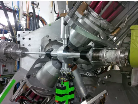
Figure 3.1: Picture of SONIC@HORUS. The setup is opened, only one hemisphere of HORUS is visible carrying half of the 14 HPGe detectors surrounding SONIC in the center. The beam line goes from the left background to the right foreground.

Figure 3.2: (a): Schematic drawing of HORUS hosting 14 HPGe detectors placed at the corners and planes of a cube. Figure taken from [27].

(b): Scheme of SONIC housing 12 Si detectors placed in 3 ring of 4 detectors each.

Figure taken from [31].

ness of 0.9mg/cm

and 1.2mg/cm

and enrichments of above 70% and above 90%

respectively. The experiment was performed in August 2016 and lasted 7 days. The targets were swapped in the middle of the beam time.

The γ -rays were registered with the HORUS [27] cube spectrometer (High e- ciency Observatory for γ -Ray Unique Spectroscopy), equipped with 14 high purity Germanium (HPGe) detectors. Figure 3.2 (a) shows a scheme of HORUS. Six detec- tors are facing the planes of an imaginary cube and eight are pointing to the corners of the cube. Six of the detectors were equipped with BGO shields. A detailed description can be found in Ref. [27].

The SONIC [31] spectrometer (Silicon Identication Chamber) contains 12 Sili- con detectors placed in 3 rings of 4 detectors each at backwards angles towards the beam line direction. The solid angle coverage in backwards direction is 9%. Figure 3.2 (b) shows a scheme of SONIC. The spectrometer houses the target frame in its center, so that back scattered particles are registered by the Si-detectors.

Figure 3.1 shows a picture of the whole setup. The opened HORUS spectrometer is shown. Only one hemisphere holding 7 HPGe detectors is visible. In the center of HORUS the closed SONIC spectrometer is placed, integrated in the beam line.

The beam direction is from left to right.

3.2.2 Data acquisition and data processing

The detector signals are preamplied and processed by Digital Gamma Finder (DGF-4C) modules made by the company XIA LLC [33]. Each module has 4 in- put channels. Particle and γ -ray detector signals are digitized by the analog to digital converters (ADC) of the DGF modules. Each input channel is associated with a veto channel, which is used to directly reject a signal, if a corresponding BGO shield is attached and triggered. After the digitalization the amplitudes of de- tector signals correspond to uncalibrated channel numbers. Several DGF modules are synchronized by distributing the clock signal of a master module to the other modules. With this equipment, the data acquisition system (DAQ) is capable of rejecting signals if a required multiplicity of detector signals is not fullled. This way single events, that do not involve at least two detector signals necessary for γγ - and pγ -coincidence experiments, can be ignored. The multiplicity requirement was set to two during the experiment of this work. A detailed description of the DAQ can be found in Ref. [34].

The listmode les written by the DAQ were processed oine by the code SO- COv2 [35]. A crucial step is setting a time window for coincident detector events.

Additionally, a calibration can be handed to the code. Specic detector types can be set as event triggers. In this work, the particle detectors were set as trigger to ensure measured coincidences were stemming from a back scattered particle i.e.

events most likely originating from the target material were processed and back-

ground noise was reduced. From these input settings, SOCOv2 sorts event les

which are then processed in a second step to build two-dimensional matrices. For

the analysis, γγ -, pγ - and γp -matrices were build. By handing gate parameter for a

specic detector type to the code, the process of building the matrices is restrained

to events within the gate. An analysis of triple events is possible this way, although

the rst gate of the building process cannot be background corrected.

3.3 Calibration

3.3.1 Energy Calibration

-0.3 -0.25 -0.2 -0.15 -0.1 -0.05 0 0.05 0.1 0.15 0.2

0 500 1000 1500 2000 keV

Residual of energy peaks to values of Kumpulainen et al. in keV

Figure 3.3: Residual of energy values of peaks used for linear calibration to energies given in the work of Kumpulainen et al. [30].

Ge-Detectors A proper calibration of an experimental setup is a vital task for the analysis of γ -ray spectra. A common procedure is the measurement of a calibration source with the used detector setup shortly before or after the conducted experiment.

This way energy values can be assigned to the counting channels of the DAQ. In this work, a

Ra calibration source was used, which is an established standard for this task [36].

Ra has a half life of 1600 years before going through an α -decay. It is the starting point of a chain of α - and β

-decays of signicantly shorter lifetimes, so that a sucient amount of γ -rays is provided from the daughter nuclei, spread over an energy range up to 3 MeV. Energy values of

Ra have been taken from [36], which also provides relative intensities for the decay chain, allowing an eciency calibration of the detector setup.

A major problem in the calibration procedure, was a gain shifting in the detector

electronics over the whole beam time. In such cases, peaks are not present in the

same channels in each subrun, but rather shift their channel number, which results

in wrong energies and broad peaks after the calibration. This problem can be taken

into account by the SOCOv2 [35] sorting code, which provides tracking of peaks

separately for each detector starting at a given channel number from subrun to

subrun. The resulting shift polynomials from this step are processed during the

sorting procedure and are combined with the calibration polynomials handed to the

code. Afterwards the energy peak of each subrun match with those of the previous subruns. Unfortunately, a gain shift also happened in the electronics during the time period between the experiment and the measurement of the calibration source. The conducted energy calibration with the

Ra source did thus not produce a satisfying assignment of energies to channels for the beam time. The spectra taken during the calibration were shifted about 2-10 keV compared to the spectra taken during the experiment. Therefore, the only detector with a nearly adequate calibration and a deviation to literature values of

Cd [1] of 0.2 keV - 0.5 keV has been taken as a reference. The quadratic calibration polynomials of the detectors had to be manually modied, so that each detector matches the peak pattern of the reference detector.

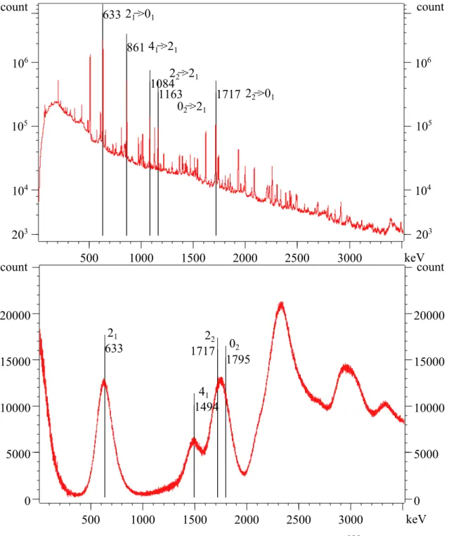
That way it was possible to obtain a rst calibration of the setup. Non-linear energy shifts could be handled by this procedure. To further improve the calibration, energy values have been taken from the work of Kumpulainen et al. [30] and a linear correction has been conducted. Figure 3.3 shows the residual of the nal calibration to energy values given in Ref. [30]. The standard deviation of that residual gives an error of 0.09 keV, a value well below the energy uncertainty of 0.3 keV given in Ref. [30]. Therefore, an error of 0.3 keV for energy values has been adopted in this work. Note however that this second calibration was not handed to the sorting code SOCOv2, but was rather applied after the data analysis. Therefore, gures showing γ -spectra in this work may not display the resulting energies presented in Table 3.1.

It is emphasized that the deviation of energy values to the literature is starting to exceed the 0.3 keV energy uncertainty of this work from ∼ 2.3 MeV upwards. As one can see from Figure 3.3, the 2370 keV ground state transition reveals the beginning of this eect by an increasing deviation to the literature. Also, Table 3.1 displays some higher energetic ground state transitions, that do not match with the level energies. Thus, to get the most valid values, γ -rays beyond ∼ 2.3 MeV have not been taken into account in the calculation process of level energies.

Si-Detectors With the Ge-detectors calibrated, the Si-detectors can be calibrated from a p γ -matrix. By gating on γ -rays that can clearly be assigned to certain level energies, a single excitation can be observed in the p-spectra, which can in turn be associated to the level energy. The FWHM of peaks in the p-spectra is typically in the range of 180 keV (Figures 3.7 and 3.10 give an impression of the energy resolution.). After the calibration, peak centroids match with level energies in a range of ± 10 keV.

3.3.2 Eciency Calibration

Germanium-detectors are not equally sensitive to γ -radiation of dierent energy. As

the probability for Compton-scattering increases with energy, the probability for a

γ -ray to deploy its full energy in the detector crystal decreases. It is also more likely

for a γ -ray to pass through the crystal without interaction, i. e. the detector is less

ecient to γ -radiation with increasing energy resulting in an under representation

of higher energetic γ -rays in the count rates. Besides this intrinsic eciency, γ -ray

detection is also inuenced by the geometry of the setup i. e. the coverage of solid

angle by detector material, which is called the geometric eciency of the setup. The

0 0.2 0.4 0.6 0.8 1 1.2 1.4 1.6

0 500 1000 1500 2000 2500

Peak volume ²²⁶Ra in % normalized to strongest literature line at 609keV

keV Fit of efficiency function without upslope at low energy

Fit of efficiency function with upslope at low energy

Figure 3.4: Fit of the detector eciency function given in [37] to peak volumes of the

Ra calibration source with relative intensities > 4% . The peak volumes have been normalized to the strongest γ -ray at 609 keV and to their relative intensity given in [36].

geometric eciency strongly inuences the overall count rate of γ -radiation. For the determination of branching ratios it is therefore crucial to determine the intrinsic eciency of the setup.

The relative (intrinsic) eciency

is determined by tting a proper function to normalized peak volumes of the

Ra calibration source. Figure 3.4 shows peak volumes (red color) normalized to the strongest line of the source (at 609.3 keV) and at the same time to their relative intensity given in Ref. [36]:

(E

) = N (E

)

I

· N (609 keV ) . (3.1)

Eciency functions from Refs. [37, 38] have been tted to the data whereas best t results were achieved with the function stemming from Ref. [37]:

(E

) = A · exp(−B · ln(E

− C + D · exp(−E · E

))). (3.2)

As can be seen from Figure 3.4, the expected upslope at low energy values could not

clearly be reproduced by the tting procedure due to the absence of data points in

that region. The X-ray shielding added to the detector fronts during the experiment

did not reduce the energy values in Figure 3.4 suciently. Dierent starting parame-

ters for the tting procedure of Equation 3.2 have produced the same outcome. The

blue curve in Figure 3.4 is the result of the tting process with a reduced χ

= 1.67 . The residual of the data point at the lowest energy of 186 keV is normally distributed to the blue curve. However, this point could also indicate the maximum of Equa- tion 3.2 if it was lying at the end of the up slope part. The purple curve displays an alternative perspective to the data points. This outcome has been produced by adding a constructed data point at (0, 0) . The t has a χ

= 1.72 .

As the lowest γ -ray in this work has an energy of 163 keV and other γ -rays are close to the potential maximum of the purple curve at ∼ 220 keV, it is of interest to get an estimate of eciency uncertainties under the assumption that the alternative t might be valid. The articial data point at (0, 0) is not unjustied from a physical point of view, as a low detector eciency can be expected at very low energy. If, hypothetically, additional X-ray shielding was placed in front of the detectors, the minimum detectable energy would rise. The constructed point of zero eciency would shift to lower values, resulting in a y-intercept of the curve. Due to the energy dependence of the γ -ray cross section, higher energetic γ -rays would be less shifted resulting in a less steep upslope. The purple curve can thus be considered as an extreme case of steep upslope at low energies.

Intensities of γ -rays have thus been calculated from both curves during the anal- ysis. The errors of the intensities of each curve include the error of the peak t and the standard deviation of residuals coming from the t of the eciency function ( 1σ condence level). The law of error propagation has been applied in this step.

The curves serve as starting points for upper and lower error limits accordingly.

The error of each of this two derived intensities is added or subtracted to the upper and lower value respectively, thereby expanding interval between these error limits.

Values for relative intensities of Table 3.1 have been calculated from the arithmetic mean of these upper and lower limits.

3.4 General data analysis methods

From the coincident measurements γγ -, p γ - and γ p-matrices were build. As a general approach to obtain γ -ray energies, a gate was set from below in a γγ -matrix, i.e, the gate was set on a transition depopulating levels fed by the transition of interest.

This yields γ -peak free of contaminating components, that can easily be tted.

Level energies have been derived by summing γ -ray energies of cascades leading to

the corresponding nal levels, though γ -rays beyond ∼ 2.3 MeV have not been used

in the sum, as discussed above. Newly discovered γ -rays have been crosschecked

by gating on them in a γ p-matrix to derive the corresponding level energy. In

return, by setting a p-gate to this level energy a coherent spectrum of transitions

belonging to the γ -cascade had to be observed. Figure 3.5 gives an impression of

this procedure, when gating in a p γ - or γ p-matrix. E.g. a γ -gate set to the 861 keV

4

→ 2

transition in a γ p-matrix results in a 1494 keV peak in the p-projection,

vise versa gating on the energy of the 4

state in a p γ -matrix gives a γ -spectrum

containing merely the 861 keV and 633 keV peaks. Some complicated combinations

of γ -multiplets made it necessary to build triple events or cubes, further on denoted

as p-gated γγ -matrices or p γγ -matrices. For the extraction of branching ratios, a

p-gate was set to the level energy in a p γ -matrix. The peak of interest was tted

in the resulting γ -projection. In case of a multiplet peak, the γ -ray energies of all components were determined before and set to xed values in the tting procedure.

In the following Section 3.5, paragraphs corresponding to level energies describe each new nding and in some cases even more complicated approaches that were made to obtain the shown results.

3.5 Experimental Results

As no γγ -angular correlation was part of the analysis, literature [1] spin assignments have been adopted in this work. Spin ranges have been assigned to newly discovered levels according to the selection rules of the deexciting γ -transitions related to the spin of the nal levels. Thereby, it was assumed, that these γ -rays have preferably an E2 - or M 1 -multipolarity. Parity changing E1 -multipolarity transitions are assumed to be possible, but present to lesser extend and only at higher energies, due to the fact, that the negative parity orbital h

has the highest energy within the 50-82 N shell among the single particle orbitals (see Figure 4.1). The same assumption was applied, when ranges of literature spin values have been constricted by classifying newly discovered transitions. Note that, although a γγ -angular correlation analysis was conducted, only spin ranges were suggested in Ref. [27] instead of concrete spins for many newly discovered levels. It seems, that the same assumptions concerning transition multipolarities, applied in this work, have also been applied in Ref. [27]

for the conrmed levels in Table 3.1. In some cases spins dierent to the literature [1] were derived in Ref. [27], which are discussed shortly in the corresponding level section.

Note that the discussion in this section excludes ndings, especially spin assign- ments coming from a new analysis of the (n, n

) -data [28]. These ndings are referred to in Section 4.1, where experimental data is compared to the shell model.

In Figure 3.5 total projections of the γγ - and p γ -coincident data are shown.

Some low energetic levels and associated γ -rays are marked in the p- and γ -spectrum

respectively. In Appendix A Table A.1 provides results of this work ordered by γ -ray

energy. Together with the γ -spectrum of Figure 3.5 an impression about the density

of peaks in the γ -spectrum can be gained, which makes the analysis challenging and

tedious.

1000 2000 3000

500 1500 2500

633 861

1084

1163 1717

10

10

10

20

count

10

10

10

20

count

keV 2

>0

4

>2

2

>0

0 10000 20000

5000 15000

0 10000 20000

5000 15000

1000 2000 3000

500 1500 2500

633

1494 1795 2

4

2

0

1717

keV

count count

Figure 3.5: Top: Total projection of the γγ -coincidence data of

Cd displayed at a logarithmic scale.

Bottom: Total projection of the p γ -coincidence data of

Cd.

Table 3.1: Results of the (p, p

γ) -experiment. Energy uncertainties are 0.3 keV.

Values marked with

are conrmed results from experiments conducted in [27], which have been published there for the rst time, but can not be found in the literature [1].

marked results found newly in this work and are not published elsewhere. Values that dier from the literature [1] are marked with

.

E

J

E

I E

J

Comments &

[ keV] [~] [ keV] [%] [ keV] [~] NNDC val. [1]

632.7 2

632.7 100 0.0 0

1493.9 4

861.2 100 632.7 2

1716.6 2

1083.9 100.0(41)

632.7 2

I

= 80(20) 1716.7 68.6(31)

0.0 0

I

= 100(15)

1795.2 0

1162.5 100 632.7 2

2104.7 4

388.0 3.12(20) 1716.6 2

610.8 100.0(41) 1493.9 4

1472.1 51.2(22) 632.7 2

2144.1 0

427.4 37.6(16) 1716.6 2

1511.5 100.0(41) 632.7 2

2252.3 (4

) 535.9

7.7(11) 1716.6 2

757.8 10.6(11) 1493.9 4

1620.0 100(5) 632.7 2

2254.1 (2

, 3

) 1621.4 100.0(42) 632.7 2

2305.1 4

811.2 100.0(41) 1493.9 4

1672.5 10.90(53) 632.7 2

2330.6 5

225.9 100.0(42) 2104.7 4

836.7 37.9(20) 1493.9 4

2347.9 (2)

1715.2 100 632.7 2

2370.5 2

575.3 33.5(15) 1795.2 0

653.9 33.2(15) 1716.6 2

1738.0 100.0(41) 632.7 2

2370.3 4.15(22) 0.0 0

2378.6 3

1745.9 100 632.7 2

2468.3 (4)

163.2

2.56(29) 2305.1 4

214.1

5.53(29) 2254.1 (2

,3

) 751.7

20.35(83) 1716.6 2

974.5 100.0(41) 1493.9 4

1835.8

24.8(12) 632.7 2

2486.1 2

− 4

381.4

4.23(33) 2104.7 4

769.4

14.52(78) 1716.6 2

992.2 39.2(19)

1493.9 4

I

= 100(30) 1853.5 100.0(42)

632.7 2

I

= 95(9)

2491.7 6

997.8 100 1493.9 4

2503.4 6

1009.5 100 1493.9 4

2561.6 0

1928.9 100 632.7 2

2566.3 2

771.4

0.24(7) 1795.2 0

849.3

0.79(7) 1716.6 2

1933.6 100.0(41) 632.7 2

E

J

E

I E

J

Comments &

[ keV] [~] [ keV] [%] [ keV] [~] NNDC val. [1]

2629.3 5

298.7 5.91(76) 2330.6 5

524.6 100.0(43) 2104.7 4

1135.4 23.8(12) 1493.9 4

2630.1 2

485.6

0.46(8) 2144.1 0

835.2

0.54(8) 1795.2 0

913.4

8.94(45) 1716.6 2

1997.4 100.0(41) 632.7 2

2629.5 7.01(33) 0.0 0

2710.8

2 − 6 1216.9

100 1493.9 4

2717.6 2

, 3 339.2

5.4(16) 2378.6 3

1000.8

17.8(53) 1716.6 2

2084.9 100(40) 632.7 2

2719.4 1, 2

2086.7 100(18) 632.7 2

J

= 1, 2

, 3 2719.3

5.91(79) 0.0 0

2792.5

2 − 6 487.3

15.58(84) 2305.1 4

687.8

3.83(33) 2104.7 4

1298.7

100.0(42) 1493.9 4

2800.6

2 − 6 495.5

53.2(29) 2305.1 4

548.1

23.6(18) 2252.3 (4

) 696.0

100.0(46) 2104.7 4

1306.8

33.3(24) 1493.9 4

2824.6 1 1029.3

5.19(35) 1795.2 0

2191.1

2.87(32) 632.7 2

2823.4 100.0(42) 0.0 0

2889.3 1, 2

518.5

1.26(11) 2370.5 2

J

= 2, 3

Hints for level doublet J

= 1 in [27]

541.6

1.07(11) 2347.9 (2)

1094.2

3.10(19) 1795.2 0

1172.7

1.90(13) 1716.6 2

2256.4 100.0(41) 632.7 2

2888.2

12.48(55) 0.0 0

2895.7

2 − 6 791.1

6.34(50) 2104.7 4

1401.8

100.0(44) 1493.9 4

2914.9

0 − 4 2282.2

100 632.7 2

2917.7 1 1122.3

8.63(58) 1795.2 0

1201.1

9.91(62) 1716.6 2

2285.4 19.3(10) 632.7 2

2916.3 100.0(43) 0.0 0

2920.6 5

1426.7 100 1493.9 4

2924.6 6

432.9 100 2491.7 6

2926.7

2 − 4 822.1

43.5(20) 2104.7 4

1210.2

9.19(54) 1716.6 2

1433.0

100.0(43) 1493.9 4

2293.6

15.47(95) 632.7 2

2936.2 2

, 3

631.1

4.22(89) 2305.1 4

E

J

E

I E

J

Comments &

[ keV] [~] [ keV] [%] [ keV] [~] NNDC val. [1]

831.1

7.66(49) 2104.7 4

1219.5

1.75(36) 1716.6 2

1442.7

41.2(20) 1493.9 4

2303.4 100.0(43) 632.7 2

2973.3 2

1178.0 5.32(34) 1795.2 0

J

= 2, 3

, 4

2340.3 100.0(42) 632.7 2

3012.6

2 − 4 1518.5

100.0(45) 1493.9 4

2380.2

23.1(19) 632.7 2

3018.8 3

, (5)

640.7

11.74(67) 2378.6 3

687.9

7.39(46) 2330.6 5

713.6

4.51(38) 2305.1 4

766.4

17.43(90) 2252.3 (4

) 1525.0 100.0(43) 1493.9 4

3020.5 2, 3

1303.8

8.09(48) 1716.6 2

2387.5 100.0(42) 632.7 2

3044.2 8

541.0 74(18) 2503.4 6

552.3 100(22) 2491.7 6

3059.5 3 1565.6 38.5(19) 1493.9 4

2426.7 100.0(44) 632.7 2

3061.2

(1), 2 593.5

9.05(98) 2468.3 (4)

1344.7

26.3(15) 1716.6 2

2428.8

100.0(49) 632.7 2

3060.8

27.3(14) 0.0 0

3073.0 2

694.2

6.17(40) 2378.6 3

J

= 2, 3

, 4 819.1

10.87(63) 2254.1 (2

,3

)

2439.6 100.0(43) 632.7 2

3071.8

4.39(32) 0.0 0

3084.3 7

592.6 100 2491.7 6

3093.0 (2

) 787.9

20.0(19) 2305.1 4

1376.3 78.5(48)

1716.6 2

I

= 100(13) 1599.1 71.2(43)

1493.9 4

I

= 35(5) 2459.9 100.0(53)

632.7 2

I

= 75(5) 3119.4

1

553.0

2.30(35) 2566.3 2

Level doublet

[39] questioned:

J

= 2

, 3

, 4

and J

= 1 558.0

9.26(64) 2561.6 0

748.6

15.7(14) 2370.5 2

1324.0

3.47(51) 1795.2 0

1402.9 20.7(12)

1716.6 2

I

= 100(13) 2486.3 100.0(45)

632.7 2

I

= 64(9) 3118.0 54.3(25)

0.0 0

I

= 100(9) 3126.4

1 − 4 747.8

4.22(12) 2378.6 3

2493.2

100.0(66) 632.7 2

3127.6 7

624.2 100 2503.4 6

3132.3

4 − 7 640.6

100.0(47) 2491.7 6

801.6

58.5(35) 2330.6 5

E

J

E

I E

J

Comments &

[ keV] [~] [ keV] [%] [ keV] [~] NNDC val. [1]

3198.1

2 − 6 1704.2

100 1493.9 4

3214.3

1 − 4 835.7

21.1(13) 2378.6 3

1497.7

100.0(43) 1716.6 2

3222.4 1 1427.3

7.8(43) 1795.2 0

2589.6

19.4(11) 632.7 2

3220.2 100.0(44) 0.0 0

3235.3 2, 3

1518.7 17.0(12)

1716.6 2

I

= 100(13) 2601.8 100.0(46)

632.7 2

I

= 19(4) 3245.5 (2

) 992.8

100.0(58) 2252.3 (4

)

1141.1 13.2(15)

2104.7 4

I

= 63(12) 1528.8 68.9(41) 1716.6 2

3244.0 93.9(63) 0.0 0

3283.6 4 − 8

780.2 100 2503.4 6

J

=

only 3285.5

1 − 4 567.7

47.7(29) 2717.6 2

,3

907.2

100.0(50) 2378.6 3

3320.4 6

691.2 100(13) 2629.3 5

828.6 41.4(77) 2491.7 6

3323.0 2

, 3

604.9

6.08(87) 2717.6 2

,3 J

= 1

, 2

, 3 1829.6

14.3(18) 1493.9 4

2689.0 100(15) 632.7 2

3328.2 2

438.8

7.16(86) 2889.3 2,3

J

= 1, 2

766.8

10.4(12) 2561.6 0

859.7

67.5(71) 2468.3 (4)

980.5 56.0(59) 2347.9 (2)

1074.3

28.4(29) 2254.1 (2

,3

) 1833.8

62.3(70) 1493.9 4

2694.9 100(12) 632.7 2

3326.9 19.3(19)

0.0 0

I

= 50(9) 3333.2

2 − 6 1027.9

46.6(57) 2305.1 4

1839.4

100.0(66) 1493.9 4

3357.5 3 − 7 1026.9 100 2330.6 5

3366.5 8

874.8 100 2491.7 6

3371.9

1 − 4 482.4

73.8(50) 2889.3 2,3

654.1

82.8(88) 2717.6 2

,3 1024.3

100.0(65) 2347.9 (2)

3392.6 1, 2

1676.0

30.9(21) 1716.6 2

J

= 2

J

= 1 Adopt.

from [27]

2757.9

60.1(30) 632.7 2

3391.4 100.0(48) 0.0 0

3427.8 2, 3

,4

1933.9

43.6(59) 1493.9 4

2793.2 100.0(44) 632.7 2

3461.2 (6

) 831.9 100 2629.3 5

3483.2

2 − 4 1112.7

100.0(45) 2370.5 2+

1989.3

31.8(20) 1493.9 4

3489.4

2 − 4 771.7

32.6(22) 2717.6 2

,3