Changing Wage Structure in India in the Post-Reform Era

(1)

Policy Research Working Paper 7426

Changing Wage Structure in India in the Post-Reform Era

1993–2011

Hanan G. Jacoby Basab Dasgupta

Development Research Group Poverty and Inequality Team September 2015

WPS7426

Public Disclosure Authorized Public Disclosure Authorized Public Disclosure Authorized Public Disclosure Authorized

(2)

Abstract

The Policy Research Working Paper Series disseminates the findings of work in progress to encourage the exchange of ideas about development issues. An objective of the series is to get the findings out quickly, even if the presentations are less than fully polished. The papers carry the names of the authors and should be cited accordingly. The findings, interpretations, and conclusions expressed in this paper are entirely those of the authors. They do not necessarily represent the views of the International Bank for Reconstruction and Development/World Bank and its affiliated organizations, or those of the Executive Directors of the World Bank or the governments they represent.

Policy Research Working Paper 7426

This paper is a product of the Poverty and Inequality Team, Development Research Group. It is part of a larger effort by the World Bank to provide open access to its research and make a contribution to development policy discussions around the world. Policy Research Working Papers are also posted on the Web at http://econ.worldbank.org. The authors may be contacted at hjacoby@worldbank.org.

This paper documents the changing structure of wages in India over the post-reform era, the roughly two-decade period since 1993. To investigate the factors underlying these changes, a supply-demand framework is applied at the level of the Indian state. While real wages have risen across India over the past two decades, the increase has been greater in rural areas and, especially, for unskilled workers. The

analysis finds that, in rural areas, the changing wage struc-

ture has been driven largely by relative supply factors, such

as increased overall education levels and falling female labor

force participation. Relative wage changes between rural and

urban areas have been driven largely by shifts in employment,

notably into unskilled-intensive sectors like construction.

(3)

Changing Wage Structure in India in the Post‐

Reform Era: 1993‐2011

By Hanan G. Jacoby

^

and Basab Dasgupta

^†

JEL codes: J21, J23, J24, J31

Keywords: Labor Supply, Labor Demand, Rural Wages in India



DECRG, World Bank, 1818 H St. NW, Washington DC 20433 (hjacoby@worldbank.org). We thank Rinku Murgai

and Ambar Narayan for helpful suggestions.

†

GWADR, World Bank (bdasgupta@worldbank.org)

(4)

I. Introduction

We investigate changes in the structure of wages in India over the post‐reform era, the roughly two‐decade period since 1993, paying particular attention to recent trends in the wages of rural workers, especially the unskilled. Poverty reduction, much of it concentrated in rural areas, has accelerated over the last few years, largely due to increased earnings from non‐agricultural wage employment (Balcazar et al. 2015). An exploration of the fine‐grained details of India’s labor market transformation will thus help us to better understand this poverty decline.

Our approach hews closely to the Supply‐Demand‐Institutions (SDI) framework pioneered by Katz and Murphy (1992) and Bound and Johnson (1992). The idea is to divide the workforce into imperfectly substitutable demographic groups; e.g., by gender, education, and age. The twist, in our case, is to also cut the data by rural/urban, recognizing that, to a large extent, rural and urban India constitute distinct labor markets, or at least are far from being perfectly integrated. Thus, our apparatus allows us to investigate, for example, changes in wages of the rural unskilled relative to their urban counterparts.

A second point of departure from conventional SDI analysis is its application at the state level, treating each Indian state (or group of states) as having separate urban and rural labor markets. A state‐level approach provides the requisite degrees of freedom for econometric analysis (see Juhn and Kim, 1999, for a related study of US states). In particular, SDI decomposes wage changes for a group into supply shifts (changing group employment shares), demand shifts (changing industrial composition biased for or against a group), and wage‐premia shifts (essentially, movements into or out of structurally low‐paying jobs). We then take the analysis a step further by investigating the key state‐level drivers of recent relative wage trends; i.e., we ask what types of supply or demand shifts were particularly influential in explaining the changing wage structure in India over the last decade.

There is a modest literature exploring India’s wage structure using data from NSS’s Employment‐Unemployment surveys. Hnatkovska and Lahiri (2013) consider rural‐urban wage convergence in India from 1983‐2009 using a model of long‐run structural transformation, but they do not decompose supply and demand factors behind the more recent wage trends. While Chamarbagwala (2006), like us, uses a supply‐demand decomposition, it is focused on the impact of trade liberalization over the earlier 1983‐99 period (see also Azam, 2010).

The organization of the paper is as follows. We begin in Section II by defining our groups

and industries and then documenting how real and relative wages in India have changed

over the past two decades. In Section III, we review the SDI framework and apply it to the

national level. Next, we turn to the state‐level SDI analysis in Sections IV and V, followed by

conclusions in Section VI.

(5)

II. Preliminaries

A. Definitions: groups and industries

We analyze three rounds of the NSS, the 50th (1993‐94), 61st (2004‐05), and 68th (2011‐

12), thus covering an 18 year span. Workers between 12 and 65 years of age are divided into 8 demographic groups, consisting of the 2x2x2 interaction of male/female, educated (completed secondary level or above)/uneducated (less than completed secondary), young (12‐29)/old (30‐65). In addition, we construct aggregates for these 8 demographic groups by sector (urban/rural), yielding 16 groups in total.

Wage earners are defined as those engaged in “gainful activities”, as recorded in their “usual principal status” in the NSS, but not self‐employed. Usual principal status also serves as our basis for categorizing individuals into industry groups below. We focus on principal status because this accounts for the preponderance of the reference period of 365 days preceding the date of survey.

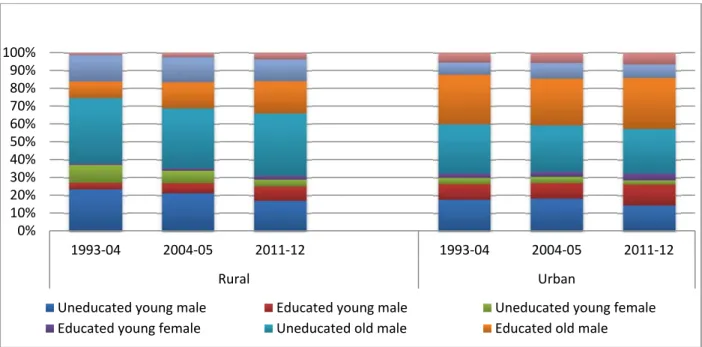
¹

Figure 1: Relative shares of demographic groups among wage earners

Figure 1 shows the extent to which each demographic group is represented among sector‐

specific wage‐earners. Of particular note is the increasing share of educated, which is much more pronounced in rural than in urban areas. Despite this trend, uneducated males remain the dominant group in rural wage labor markets.

1

Subsidiary status is much more temporary in nature and, as NSSO suggests, only about 1.3% in the rural and 0.1%

in the urban areas had participated in two subsidiary economic activities during the period of one year before the date of survey in round 55 (NSSO, 2008).

0%

10%

20%

30%

40%

50%

60%

70%

80%

90%

100%

1993‐04 2004‐05 2011‐12 1993‐04 2004‐05 2011‐12

Rural Urban

Uneducated young male Educated young male Uneducated young female

Educated young female Uneducated old male Educated old male

(6)

We next define five broad “industry” or occupational categories: (1) agriculture (inclusive of forestry and fishery); (2) construction; (3) manufacturing (inclusive of mining and utilities);

(4) Professional (including public administration); (5) services (inclusive of wholesale/retail trade and domestic service).

²

SDI analyses using developed country data, and even Chamarbagwala’s (2006) study of urban Indian wages, typically use a much more fine‐

grained industrial classification. However, sample size considerations constrain us to only five. Rural India is predominately agricultural; manufacturing, in particular, has until very recently accounted for much less than ten percent of rural employment. Given the typical NSS sample, there would simply not be enough wage‐earners in each category to support a very detailed classification. This concern is only reinforced in our state‐level analysis, where state‐wise wage‐earner samples are much smaller.

1993‐94 2004‐05 2011‐12

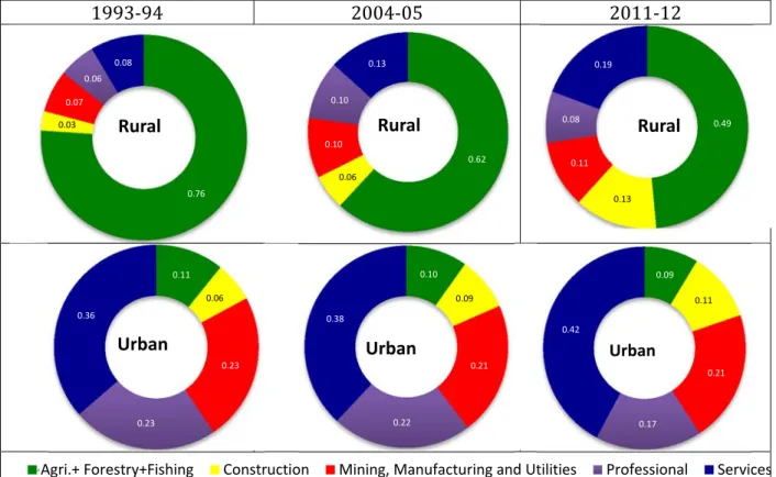
Figure 2: Share of industries in Rural‐Urban employment

2

See Appendix Table B.1 for details on how industry codes were harmonized across NSS rounds.

0.76 0.03

0.07 0.06

0.08

Rural

0.62 0.06

0.10 0.10

0.13

Rural

^0.49

0.13 0.11 0.08

0.19

Rural

0.11 0.06

0.23

0.23 0.36

Urban

0.10 0.09

0.21

0.22 0.38

Urban

0.09 0.11

0.21

0.17 0.42

Urban

Agri.+ Forestry+Fishing Construction Mining, Manufacturing and Utilities Professional Services

(7)

Patterns of industrial employment have changed rather dramatically in rural India over the past two decades. As seen in Figure 2, from around three‐quarters in the early‐1990s, the share of rural labor employed in agriculture had, by 2011, declined to around one‐half. The two main rural growth industries are services and construction, with the latter’s employment share more than quadrupling over the last two decades. By contrast, the urban picture is one of relative stasis, with more modest expansions of services and construction over the same period.

Rural Urban

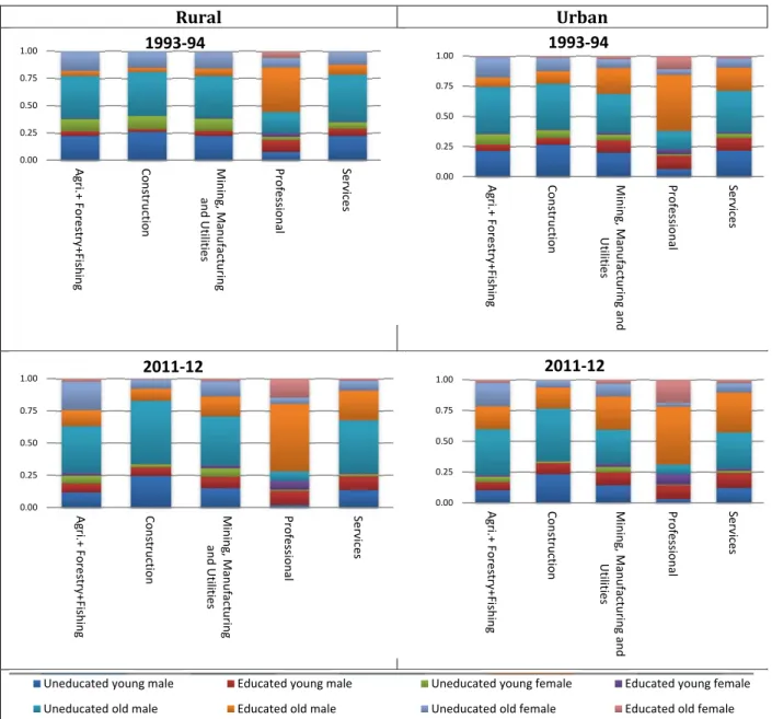
Figure 3: Share of demographic group in each industry

0.00 0.25 0.50 0.75 1.00

Agri.+ Forestry+Fishing Construction Mining, Manufacturingand Utilities Professional Services

1993‐94

0.00 0.25 0.50 0.75 1.00

Agri.+ Forestry+Fishing Construction Mining, Manufacturing andUtilities Professional Services

1993‐94

0.00 0.25 0.50 0.75 1.00

Agri.+ Forestry+Fishing Construction Mining, Manufacturingand Utilities Professional Services

2011‐12

0.00 0.25 0.50 0.75 1.00

Agri.+ Forestry+Fishing Construction Mining, Manufacturing andUtilities Professional Services

2011‐12

Uneducated young male Educated young male Uneducated young female Educated young female Uneducated old male Educated old male Uneducated old female Educated old female

(8)

Representation of the 8 demographic groups in each industry is shown for both rural and urban areas in Figure 3. Educated workers, obviously, predominate in the professions, whereas wage‐jobs in rural construction are largely held by unskilled males, even more so than in agriculture and quite substantially more so than in services. Both rural and urban areas have seen a gradual up‐skilling of the workforce over the past two decades, across all industrial sectors.

B. Changes in real wages

I nformation on weekly wage earnings and days worked per week is available for regular and casual workers. In the case of those who perform multiple jobs in the week, we calculate average daily wages by dividing weekly wage income from all sources by total number of days worked. To compute real wages, we use the state‐level Consumer Price Index for Agriculture (CPI‐AL) and Industrial Workers (CPI‐IW). Originally, the CPI‐AL was available with base‐year 1986‐87 and CPI‐IW with base‐year 1982. We converted these indices to have a uniform base‐year 2004‐05. CPI‐AL is used to deflate wages in rural areas and CPI‐

IW in urban India. Because these deflators are not available for some of the small states, we used available information for larger states either adjacent to them or from which they had been split (see Appendix Table B.2 for details on the CPI calculation for the smaller states).

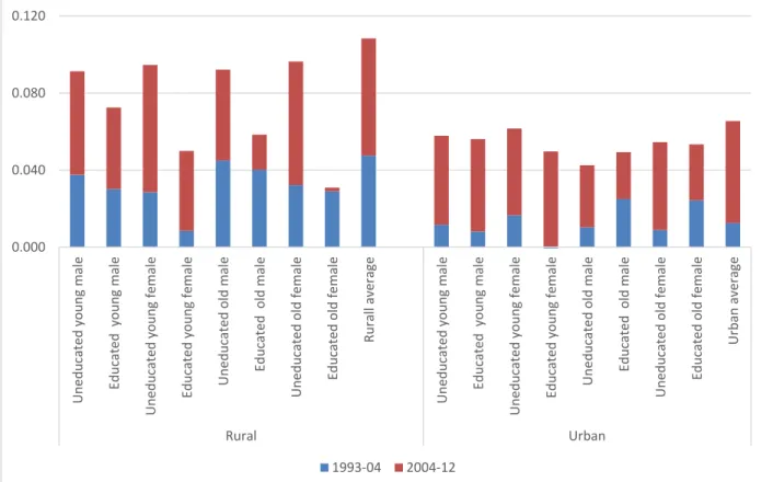
Figure 4: Annual average real wage changes by demographic group

0.000 0.040 0.080 0.120

Unedu cated young ma le Educated youn g male Unedu cated young fe m ale Educated young fe male Unedu cated old ma le Educated old male Unedu cated old fe m ale Educated old fem ale Rur al l ave rage Unedu cated young ma le Educated youn g male Unedu cated young fe m ale Educated young fe male Unedu cated old ma le Educated old male Unedu cated old fe m ale Educated old fem ale Ur ban ave ra ge

Rural Urban

1993‐04 2004‐12

(9)

Mean annualized changes in log real wages by group are shown in Figure 4 across each of the two sub‐periods. Evidently, wages have been rising in real terms over the past two decades for all groups and especially in rural areas. There has also been a marked acceleration in wage‐growth in recent years, most pronounced in urban India as well as among the unskilled (those with less than secondary education). Looking across states (Figure 5), we see big real‐

wage gains for unskilled workers in the south and east of the country, with W. Bengal being a notable exception. The remainder of our analysis will largely ignore this overall rising‐tide to focus on why some “boats” have risen faster than others.

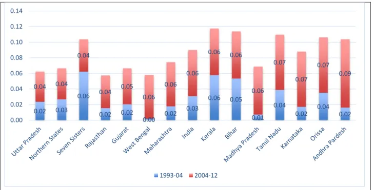
Figure 5: Annual average real wage changes for unskilled labor by state

C. Changes in relative wages within and across sectors

For ease of presentation under the first major column heading of Table 1, we aggregate mean relative wage changes across pairs of demographic groups using the respective (base‐year) shares of wage‐earners as weights. Thus, for example, the change in the wage for rural educated males relative to rural uneducated males is computed as a weighted average of the corresponding mean wage changes for old and young rural males in each of these educational categories.

0.02 0.03 0.06

0.02 0.02

0.00 0.02 0.03

0.06 0.05 0.01

0.04 0.02 0.04 0.02 0.04 0.04

0.04 0.04 0.05 0.06

0.06 0.06

0.06 0.07

0.07 0.07

0.09 0.00 0.02 0.04 0.06 0.08 0.10 0.12 0.14

1993‐04 2004‐12

(10)

Table 1: SDI decomposition of relative wage changes within rural and urban India

The first two rows of Table 1 (denominated in log changes) indicate that the wages of uneducated rural workers rose relative to those of educated rural workers (hence the negative sign) for both males and females. Much of these relative gains occurred in the most recent decade (2004‐11). Note that the urban unskilled also experienced relative wage gains in the second period, but not quite as much as their rural counterparts. Overall, rural females (especially the unskilled) gained ground on rural males in the last decade.

Table 2: SDI decomposition of relative wage changes between rural and urban India

Looking across the urban‐rural divide in Table 2, the striking pattern is wage convergence, albeit skewed toward the unskilled. Overall, wages for uneducated males rose by around 47% relative to their urban counterparts; the corresponding figure for uneducated females is 37%. However, much of these gains occurred in the earlier decade of the post‐reform era, especially for males. Similar, but substantially smaller, relative gains were experienced by educated rural workers. Aggregating across groups, rural wages rose a modest 9% relative to urban wages over the last decade, following a 27% increase in the first decade.

1993-94 to 2004-05

2004-05 to 2011-12

1993-94 to 2011-12

1993-94 to 2004-05

2004-05 to 2011-12

1993-94 to 2011-12

1993-94 to 2004-05

2004-05 to 2011-12

1993-94 to 2011-12

1993-94 to 2004-05

2004-05 to 2011-12

1993-94 to 2011-12

Educated/uneducated Male -0.09 -0.24 -0.33 0.50 0.41 0.91 -0.29 -0.37 -0.64 -0.08 0.03 -0.01

Female -0.10 -0.31 -0.41 0.82 0.70 1.51 -0.15 -0.03 -0.27 -0.07 -0.08 -0.09

Old/Young Male 0.10 -0.06 0.04 0.11 0.30 0.41 0.25 0.11 0.38 0.00 -0.07 -0.07

Female 0.05 -0.03 0.02 0.37 0.38 0.75 0.07 0.00 0.09 -0.06 0.04 -0.02

Male/Female 0.13 -0.15 -0.01 -0.06 0.34 0.28 0.28 0.31 0.47 0.41 -0.13 0.11

Educated/uneducated Male 0.11 -0.13 -0.03 0.07 0.32 0.38 -0.06 -0.11 -0.17 -0.22 0.01 -0.15

Female 0.04 -0.17 -0.13 -0.03 0.43 0.40 -0.01 -0.02 -0.04 -0.23 -0.05 -0.19

Old/Young Male 0.10 -0.16 -0.06 0.07 0.24 0.32 0.00 -0.05 -0.05 -0.14 -0.08 -0.19

Female 0.01 -0.16 -0.15 0.13 0.12 0.25 0.00 -0.01 0.00 -0.13 -0.02 -0.12

Male/Female 0.03 -0.14 -0.11 -0.17 0.15 -0.02 0.02 0.02 0.02 0.25 -0.07 0.05

Urban/Rural -0.27 -0.09 -0.36 0.28 0.20 0.48 -0.35 -0.24 -0.60 -0.08 -0.12 -0.17

Relative wage Supply Demand Institution

1993-94 to 2004-05

2004-05 to 2011-12

1993-94 to 2011-12

1993-94 to 2004-05

2004-05 to 2011-12

1993-94 to 2011-12

1993-94 to 2004-05

2004-05 to 2011-12

1993-94 to 2011-12

1993-94 to 2004-05

2004-05 to 2011-12

1993-94 to 2011-12

Urban / RuraL Educated Male -0.17 0.01 -0.16 -0.38 -0.20 -0.57

‐0.22 ‐0.11 ‐0.30

-0.21 -0.12 -0.26

Female -0.07 -0.02 -0.09 -0.73 -0.25 -0.99

‐0.03 ‐0.02 ‐0.05

-0.08 -0.12 -0.18

Urban/ Rural uneducated Male -0.37 -0.10 -0.47 0.05 -0.10 -0.05

‐0.45 ‐0.37 ‐0.77

-0.07 -0.10 -0.13

Female -0.21 -0.16 -0.37 0.12 0.01 0.13

‐0.17 ‐0.04 ‐0.28

0.08 -0.15 -0.08

Urban /Rural old Male -0.29 -0.09 -0.38 0.06 0.01 0.07

‐0.52 ‐0.37 ‐0.89

-0.19 -0.10 -0.22

Female -0.16 -0.12 -0.29 0.05 0.14 0.19

‐0.19 ‐0.04 ‐0.32

0.00 -0.17 -0.16

Urban / Rural Young Male -0.28 0.00 -0.28 0.10 0.07 0.16

‐0.27 ‐0.22 ‐0.46

-0.06 -0.09 -0.11

Female -0.12 0.00 -0.12 0.29 0.40 0.69

‐0.13 ‐0.03 ‐0.23

0.06 -0.12 -0.06

Urban/Rural Male -0.35 -0.08 -0.44 0.09 0.00 0.09

‐0.43 ‐0.32 ‐0.73

-0.15 -0.10 -0.19

Female -0.25 -0.09 -0.34 0.20 0.19 0.39

‐0.17 ‐0.04 ‐0.28

0.01 -0.16 -0.13

Urban/Rural -0.27 -0.09 -0.36 0.28 0.20 0.48

‐0.35 ‐0.24

-0.60 -0.08 -0.12 -0.17

Relative wage Supply Demand Institution

(11)

III. Supply, Demand, Institutions

A. Conceptual framework

Suppose we have a CES production function for aggregate output that depends on just two types of labor (ignore capital), types a and b. Katz and Autor (1999), e.g., show that

log , (1)

where are wages for type i in time t, is an index of relative demand shifts favoring group a, and is an index of relative supply shifts favoring group a. The parameter represents the aggregate elasticity of substitution in production between labor of type a and b. A key implication of the model is that only net demand shifts (i.e., net of supply shifts) matter for relative wages. Differencing equation (1) over time, using the notation ∆x x x , delivers

∆log ∆ ∆ . (2)

Thus, on the left‐hand side of equation (2) we have a difference‐in‐difference in mean log‐

wage for two groups over time.

³

These diff‐in‐diffs are precisely what is reported in Tables 1 and 2 for, respectively, within and between sector contrasts.

We may write the relative supply for group i in sector s at time t as

log (3)

where is the group’s employment in the sector and is total employment in the sector.

Note that employment includes self‐employment in agriculture or in a household enterprise and hence the employed are a much larger set than wage‐earners, especially in the rural sector. Shifts in supply, ∆ , are assumed to be predetermined; that is, not caused by changes in relative wages. In the state‐level analysis we will have the opportunity to test this assumption.

3

With more than two types of imperfectly substitutable labor, the change in relative wages between any two

groups will also depend on how each of their net demands shift relative to that of the other groups. For

simplicity, our analysis ignores such cross‐price effects; i.e., we implicitly assume that the matrix of elasticities

of complementarity is diagonal.

(12)

Theoretically consistent measurement of demand shifts is a complicated issue (see Katz and Autor, 1999; Bound and Johnson, 1992). We follow Juhn and Kim (1999), who use the between (industrial) sector demand shift measure of Katz and Murphy (1992),

⁴

∆ ∑ ∆log (4)

where indexes industry. So, the first term in the sum is the share of demographic group in industry ’s employment and the second term is the growth rate in the share of industry employment in overall sectoral employment. Intuitively, ∆ is larger when demographic group (initially) predominates in relatively fast‐growing industries. As with supply shifts, ∆ is taken as exogenous with respect to changes in relative wage structure;

again, this is testable.

The “institutions” component of SDI boils down to allowing for industry wage premia. A wage premium measures the extent to which a given type of worker (demographic group) is paid more (or less) when working in a particular industry. Labor market institutions matter insofar as wages are not determined solely by the interaction of skill endowments and skill prices—i.e., by the competitive market for skills. A salient example in the case of India is agricultural labor. On average, jobs in agriculture pay around a‐third less than those outside of agriculture, holding location and type of worker constant. Why this premium arises is beyond the scope of the present investigation, but it may have something to do with the fact that a higher proportion of agricultural than nonagricultural workers in India are hired on a casual daily basis (see Appendix Table B.3 for details).

Following Bound & Johnson (1992), then, let

log log ∑ (5)

where is the competitive market wage given group skills, is the industry wage premium for group at time , and ⁄ is the proportion of group workers in industry . Based on estimated from wage regressions, the institutions index (∆ ) for group is the change in the entire wage‐premium term or

∆ ∑ ∆ ∆ (6)

Returning to the case of the negative wage premium in India’s agricultural sector, we can see that a group with a higher ∆ is one which is moving out of agriculture relatively quickly.

4

Another measure of demand shifts involves a weighted average of within industry changes in group employment

shares, but we do not focus on it here for reasons discussed in the Appendix.

(13)

Comparison of group‐shares across NSS rounds, as shown in Figure 6, indicates that uneducated rural males (young and old) are shifting out of agriculture most rapidly.

Figure 6: Industry share of employment by demographic group

B. All‐India decomposition

SDI metrics at the national level are reported under, respectively, the second, third and fourth major column headings of Table 1. So, why did the wages of educated workers decline relative to the wages of uneducated workers in rural India? First off, there was a substantial increase in relative supply of educated workers, especially for females, spread rather evenly across the two sub‐periods. Meanwhile, relative demand for educated workers fell, especially for males. And, finally, there were modest declines in the institutions index for educated relative to uneducated workers. In other words, uneducated workers moved out of (low‐paid) agricultural labor faster than educated workers. Similar, but less pronounced, patterns are seen for educated vs. uneducated workers in urban India (rows 6 and 7).

In Table 2, we compute urban vs. rural SDI changes. Focusing on unskilled labor, we see that shifts in relative supply were not a decisive factor behind the wage gains of uneducated workers vis‐a‐vis the educated. There were, however, big drops in relative demand for

0%

25%

50%

75%

100%

Uneducated Young Male Educated Young Male Uneducated Young Female Educated Young Female Uneducated Old Male Educated Old Male Uneducated Old Female Educated Old Female Uneducated Young Male Educated Young Male Uneducated Young Female Educated Young Female Uneducated Old Male Educated Old Male Uneducated Old Female Educated Old Female

Rural Urban

1993‐94

0%

25%

50%

75%

100%

Uneducated Young Male Educated Young Male Uneducated Young Female Educated Young Female Uneducated Old Male Educated Old Male Uneducated Old Female Educated Old Female Uneducated Young Male Educated Young Male Uneducated Young Female Educated Young Female Uneducated Old Male Educated Old Male Uneducated Old Female Educated Old Female

Rural Urban

2011‐12

Agri.+ Forestry+Fishing Construction Mining, Manufacturing and Utilities Professional Services

(14)

unskilled male labor in urban areas, with smaller declines in the case of females. The institutions index also moved against the urban unskilled. The story of wage gains by the rural unskilled relative to their urban counterparts is, therefore, one of changing patterns of industrial employment rather than one of changing relative supplies (as was the case within the rural sector).

IV. State‐level SDI Analysis

We now compute changes in mean log wages, ∆ , ∆ , and ∆ separately for each major state or group of adjacent states.

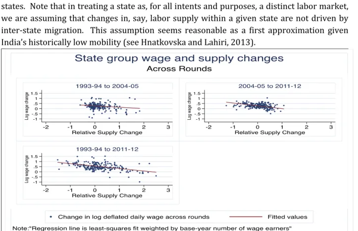
⁵

Our “data set”, therefore, consists of 448 = 2 x 2 x 8 x 14 observations for 2 decadal intervals, 2 sectors (rural/urban), 8 demographic groups, and 14 states. Note that in treating a state as, for all intents and purposes, a distinct labor market, we are assuming that changes in, say, labor supply within a given state are not driven by inter‐state migration. This assumption seems reasonable as a first approximation given India’s historically low mobility (see Hnatkovska and Lahiri, 2013).

Figure 7: Bivariate relationship between state/group wage changes and supply shifts

5

State groups consist of Chhattisgarh with Madhya Pradesh (called Madhya Pradesh); Uttaranchal with UP (called Uttar Pradesh); Jharkhand with Bihar (called Bihar); Seven Sisters in the Northeast with Sikkim (called seven sisters); Goa, D &

N Havelli, D& Diu with Maharashtra; A&N Island with West Bengal (called West Bengal); Lakshadweep with Kerala (called

Kerala) and Pondicherry with Tamil Nadu (called Tamil Nadu). Finally, Haryana, Punjab, Himachal Pradesh, Delhi, and

Chandigarh and combined into Northern states.

(15)

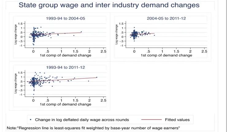
Figure 8: Bivariate relationship between state/group wage changes and demand shifts.

Bivariate scatterplots (fig. 7) reveal that increases in supply are strongly associated with wage declines in each period. Increases in demand, by contrast, are associated with wage increases (fig. 8). This is all as it should be, but to properly assess the SDI framework we need to control for both supply and demand shifts simultaneously.

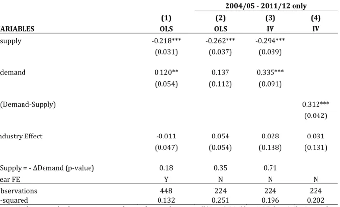
To do so, we run a series of regressions of state mean log‐wage changes on the SDI shift variables. The first such regression, shown in Table 3, uses the full dataset, thus including log‐wage changes between 1993‐2004 and 2004‐2011. Among the independent variables is a dummy for the second decadal change. Results in the first column of Table 3 show that increases in supply lead to lower wages, conditional on the demand shift. Likewise, increases in demand increase wages, conditional on the supply shift. Moreover, we cannot reject the null hypothesis that the coefficient on supply is equal to minus the coefficient on demand;

i.e., that only net demand shifts matter for wages (cf., equation (1)).

(16)

Table 3: Regression Analysis

2004/05 ‐ 2011/12 only

(1) (2) (3) (4)

VARIABLES OLS OLS IV IV

Δsupply ‐0.218* ‐0.262* ‐0.294***

(0.031) (0.037) (0.039)

Δdemand 0.120 0.137 0.335*

(0.054) (0.112) (0.091)

Δ(Demand‐Supply) 0.312***

(0.042)

Industry Effect ‐0.011 0.054 0.028 0.031

(0.047) (0.054) (0.138) (0.131)

ΔSupply = ‐ ΔDemand (p‐value) 0.18 0.35 0.71

Year FE Y N N N

Observations 448 224 224 224

R‐squared 0.132 0.251 0.196 0.202

Notes: Robust standard errors in parentheses clustered on state ( p<0.01, p<0.05, * p<0.1). Dependent* variable in all regression is mean log wage change of demographic group in state.

Next, we address the simultaneity between wage changes on the one hand and demand and/or supply shifts on the other. Do ∆ , ∆ , and, for that matter, ∆ cause wages to change, or is it the other way around? Arguably, the supply of skills and the structure of industrial employment are slow to adjust and may reasonably be thought of as predetermined. However, to test this proposition, we instrument ∆ , ∆ and ∆ by their lagged values ∆ , ∆ and ∆ . The idea here is that lagged changes reflect long‐run trends, uncontaminated by contemporaneous wage shocks. Of course, using lags as instruments requires us to drop the first decadal change, which corresponds to half our sample. Hence, in column 2 we replicate our original OLS specification on the sample of second‐decadal changes, with very similar results. IV estimates are shown in column 3.

There is little evidence of endogeneity bias; to be sure, the coefficient on demand shifts more

than doubles from its OLS magnitude, but this could be due to chance. And, the null

hypothesis of the SDI framework fares extremely well in this specification. Thus, in column

(4), we report the same IV specification but with the SDI restriction imposed, which is to say

that only net demand shifts ∆ ∆ are now included along with ∆ . In all

specifications, the coefficient on the institutions index ∆ is not significantly different from

(17)

zero. Finally, we run the same set of regressions with state fixed effects and obtain very similar results (see Appendix Table B.4).

V. SDI Drivers across States

The diagnostics of the previous section suggest that the SDI framework does a reasonably good job explaining wage growth of the past decade across both demographic groups and states. But what are the key structural trends underlying these changes? Five candidates for consideration are: (1) Urbanization; (2) NREGA; (3) the rural construction “boom”; (4) falling rural female LFP; (5) Rising agricultural prices.

We begin by predicting log‐wage changes from 2004‐2011 for each group x state observation using the results in Table 3, column 4; i.e.,

∆ ∆ ∆ ∆ . (7)

Next, we construct predicted differences‐in‐differences across groups i and j within a sector as follows

∆ ∆ ∆ ∆ (8)

or across sectors within group i using

∆ ∆ ∆ ∆ , (9)

where subscripts u and r denote, respectively, urban and rural. Finally, we examine the bivariate associations between the predicted D‐in‐Ds and each of the five structural wage drivers mentioned above.

A. Within rural India

We look first at rural areas and, in particular, at wages of educated rural workers (old/young and male/female taken together) relative to uneducated. Each panel of figure 9 shows a scatterplot of ∆

_,

∆ against a relevant driver. Having now aggregated wage changes across all 8 demographic groups, we end up with 14 data points, which is to say one

∆

_,

∆ for each state‐group.

(18)

Consider the change in the employment share of construction in rural areas of each of the 14 state‐groups. The top left panel of Figure 9 shows that higher construction shares are strongly positively associated with the predicted growth in wages for the uneducated relative to educated. Indeed, differences in construction industry growth explain about two‐thirds of the variation in the relative wage growth predicted by the SDI framework. The same exercise using the rural services share, an industry which also employs significant numbers of unskilled workers and which also expanded in relative terms over the last decade, shows a similar pattern but a weaker association with wages. In sum, the rural construction boom appears to have been an important, if not the main, driver of unskilled relative wage‐growth within rural India.

Figure 9: Drivers of changes in educated vs. uneducated wages within rural India

It is interesting to contrast the labor market impacts of the above compositional shifts to those of NREG (National Rural Employment Guarantee). Phase‐in of NREG began at around the mid‐point of our 2004‐2011 window. Analyses of NSS data preceding the 68

^th

(2011‐12) round provide mixed evidence as to the rural wage impacts of NREG expansion (see Azam, 2012; Zimmerman, 2013; Imbert and Papp, 2015). However, NSS68, for the first time, provides individual level data on NREG registration (job‐card holding) and take‐up (i.e., NREG employment in the last 12 months). This allows us to construct, for each state, the

Northern States

Rajasthan

Uttar Pradesh

Bihar West Bengal

Orissa

Madhya Pradesh Gujarat

Maharashtra

Andhra Pradesh

Karnataka Kerala

Tamil Nadu

Seven Sisters R-sq=.66

-.35-.3-.25-.2-.15

.4 .6 .8 1

diff. log rural construction share 68-61

Northern States

Rajasthan Uttar Pradesh

Bihar West Bengal

Orissa

Maharashtra

Andhra Pradesh

Karnataka Kerala

Tamil Nadu

-.35-.3-.25-.2-.15

.2 .3 .4 .5 .6

diff. log rural services share 68-61

Northern States Rajasthan

Uttar Pradesh

Bihar West Bengal

Orissa

Madhya Pradesh

Gujarat

Maharashtra

Andhra Pradesh

Karnataka Kerala

Tamil Nadu

Seven Sisters

R-sq=.02

-.35-.3-.25-.2-.15

-.3 -.2 -.1 0

diff. share NREG job-card ed/uned 68

Uttar Pradesh

Bihar West Bengal

Orissa

Maharashtra

Andhra Pradesh

Karnataka Kerala

Tamil Nadu

Seven Sisters

R-sq=.04

-.35-.3-.25-.2-.15

-.3 -.2 -.1 0

diff. share NREG worker ed/uned 68

diff. log rel. wage ed/uned 68-61 Fitted values

(19)

proportion of each demographic group that are job‐card holders or who have worked in NREG.

Figure 10: State‐wise NREG participation in rural India, 2011‐12.

Figure 11: Group‐wise NREG participation in rural India, 2011‐12.

Looking across state‐groups in figure 10, there are huge differences in NREG registration rates, with Rajasthan and MP topping the list, although rates of participation in this massive public works program are actually highest in the far east of India (“Seven Sister” states). Also relevant for our analysis is the large registration and participation gap between the educated and uneducated, with much higher NREG involvement among the latter (figure 11). Thus, we have in the two bottom panels of figure 9, plots of the predicted log‐wage D‐in‐D against the state‐wise differences in NREG participation shares (job‐card on the left; worker on the

0.13 0.31

0.15 0.11

0.30

0.17 0.23

0.06 0.04

0.27

0.06 0.14

0.28 0.41 0.24

0.79

0.21 0.21 0.52

0.36 0.72

0.22 0.15 0.48

0.14 0.24

0.39 0.53

0.00 0.20 0.40 0.60 0.80 1.00

Northern States Rajasthan Uttar Pradesh Bihar West Bengal Orissa Madhya Pradesh Gujarat Maharashtra Andhra Pradesh Karnataka Kerala Tamil Nadu Seven Sisters

Share of rural labor force working in NREG Share of rural labor force holding NREG job card

0.16 0.10

0.30

0.17 0.21

0.10

0.40

0.18

0.29 0.23

0.63

0.37 0.39

0.18

0.74

0.33

0.00 0.20 0.40 0.60 0.80 1.00

Below Secondary

Secondary and up

Below Secondary

Secondary and up

Below Secondary

Secondary and up

Below Secondary

Secondary and up

Male Female Male Female

Young Old

Rural

Share of rural labor force working in NREG Share rural labor force holding NREG job card

(20)

right) between educated and uneducated groups. Given Figure 11, all of the NREG share differences are negative (educated have lower registration and take‐up than uneducated).

What we do not see is much of a relationship between NREG participation and wage growth (the slopes are positive, but the R

²

s are essentially zero). Put differently, states in which NREG has (presumably) expanded relative employment opportunities for unskilled labor more do not appear to have experienced differential growth in net demand for unskilled labor. This is, of course, not to say that NREG has been ineffectual as a safety‐net for the poor, only that it is evidently too small of a labor market intervention to have detectable general equilibrium effects.

⁶

Next, using the same approach, we consider what has been driving changes in relative wages of men versus women in rural India over the last decade. In this case, we compute

∆

_,

∆ by aggregating wage changes for all male (m) and female (f) demographic groups within the rural sector of each state. Here we introduce another potentially relevant factor, the change in female labor force participation (LFP). Figure 12 shows massive declines in female LFP in rural areas of most states, whereas figure 13 shows much more muted ones in the corresponding urban areas.

Figure 12: Female labor force participation in rural India

6

We have done a similar analysis using “raw”, as opposed to predicted (by SDI), wage changes with the same

result.

0.00 0.25 0.50 0.75 1.00

Female LFPR

1993‐94 2004‐05 2011‐12

(21)

Figure 13: Female labor force participation in urban India

The top left panel of figure 14 provides striking confirmation that this recent movement of women out of the rural labor force explains much of the predicted increase in their wages relative to those of men; the R

²

of the associated bivariate regression is 0.84. By contrast, changes in the rural construction share (top right panel) or in women’s participation in NREG relative to men’s (bottom panels) explain next to nothing.

Figure 14: Drivers of changes in male vs. female wages within rural India.

0.00 0.25 0.50 0.75 1.00

Female LFPR

1993‐94 2004‐05 2011‐12

Northern States

Rajasthan Uttar Pradesh

Bihar

West Bengal

Orissa Madhya Pradesh

Gujarat

Maharashtra Andhra Pradesh

Karnataka

Kerala

Tamil Nadu Seven Sisters

R-sq=.84

-.2-.10.1.2

-1 -.8 -.6 -.4 -.2 0

diff. log female LFP 68-61

Northern States

Rajasthan

Uttar Pradesh

Bihar West Bengal

Gujarat

Karnataka Kerala

Tamil Nadu

Seven Sisters

R-sq=0

-.2-.10.1.2

.4 .6 .8 1

diff. log rural construction share 68-61

Northern States

Rajasthan

Uttar Pradesh

Bihar West Bengal

Gujarat Maharashtra Andhra Pradesh

Karnataka Kerala

R-sq=0

-.2-.10.1.2

-.8 -.6 -.4 -.2 0

diff. share NREG job-card male/fem 68

Northern States

Rajasthan

Uttar Pradesh

Bihar West Bengal

Gujarat Maharashtra Andhra Pradesh

Karnataka Kerala

R-sq=0

-.2-.10.1.2

-.6 -.4 -.2 0

diff. share NREG worker male/fem 68

diff. log rel. wage male to female 68-61 Fitted values

(22)

B. Urban vs. rural India

In the remainder of our analysis, we contrast urban and rural wage changes for unskilled labor. In particular, we use equation (9) to compute ∆ ∆ separately for uneducated males (figure 15) and for uneducated females (figure 16). On the x‐axis in each panel in the next two figures is the urban‐rural difference in log shares of construction employment (top left), services employment (top right), and female LFP (as a share of all females of working age). The bottom right panel of each of the figures considers the change in the urban (state) population share between the 2001 and 2011 population censuses (see figure B.1 in the appendix).

Figure 15: Drivers of changes in urban vs. rural wages for males.

Uttar Pradesh

Bihar

West Bengal Orissa

Madhya Pradesh

Gujarat

Karnataka

Kerala Tamil Nadu

-.12-.1-.08-.06-.04

-1 -.8 -.6 -.4 -.2

diff. log rel. urb/rur construction share 68-61

Uttar Pradesh Bihar

West Bengal Orissa

Karnataka Kerala Tamil Nadu

-.12-.1-.08-.06-.04

-.4 -.3 -.2 -.1

diff. log rel. urb/rur services share 68-61

Uttar Pradesh

Bihar

West Bengal Orissa

Karnataka Kerala

Tamil Nadu

Seven Sisters

R-sq=.04

-.12-.1-.08-.06-.04

0 .1 .2 .3 .4

diff. log rel. urb/rur female LFP 68-61

Uttar Pradesh Bihar

West Bengal Orissa

Maharashtra

Andhra Pradesh

Karnataka

Kerala Tamil Nadu

Seven Sisters

R-sq=.13

-.12-.1-.08-.06-.04

0 .2 .4 .6

Inter-censal urban pop. share growth

DD log-wage uneducated male urb/rural-68/61 Fitted values

(23)

Figure 16: Drivers of changes in urban vs. rural wages for females.

For males, the construction sector stands out as the key relative wage driver, with higher construction growth strongly associated with higher wage growth (R

²

=0.34), whereas for females the corresponding association is actually negative, albeit weak (R

²

=0.05). Relative growth in the service sector, by contrast, bears little relationship to relative wage changes for either males or females. As for female LFP, we again see a strong correlation with wage growth. In states where women have withdrawn from the labor force faster in the countryside than in cities, rural wages of females have risen faster than urban wages (R

²

=0.31), a pattern essentially absent with respect to male wages (R

²

=0.04).

Next, we ask whether the growth of cities has in and of itself led to changes in SDI at the state level. By far the fastest urbanization over the last decade occurred in Kerala, which is clearly an outlier in the bottom right panels of figures 15 and 16. Nevertheless, even with Kerala excluded, the story is clear. Faster urbanization is associated with greater urban wage growth relative to rural areas for both genders, but especially for females. Moreover, this latter effect is not driven merely by correlation between falling female LFP and urbanization;

it survives virtually intact after controlling for the relative change in female LFP. Thus, it appears that in rapidly urbanizing states the demand for female labor, as reflected in their wages, has been growing faster in cities than in the countryside.

Uttar Pradesh

Bihar West Bengal

Orissa

Maharashtra Andhra Pradesh Karnataka

Kerala

Tamil Nadu

-.1-.050.05

-1 -.8 -.6 -.4 -.2

diff. log rel. urb/rur construction share 68-61

Uttar Pradesh

Bihar

West Bengal Orissa

Karnataka

Kerala

Tamil Nadu

-.1-.050.05

-.4 -.3 -.2 -.1

diff. log rel. urb/rur services share 68-61

Uttar Pradesh

Bihar West Bengal

Orissa

Karnataka Kerala

Tamil Nadu

-.1-.050.05

0 .1 .2 .3 .4

diff. log rel. urb/rur female LFP 68-61

Uttar Pradesh

Bihar West Bengal

Orissa Madhya Pradesh Gujarat

Maharashtra

Andhra Pradesh Karnataka

Kerala

Tamil Nadu

Seven Sisters

R-sq=.41

-.1-.050.05

0 .2 .4 .6

Inter-censal urban pop. share growth

DD log-wage uneducated fem. urb/rural-68/61 Fitted values

(24)

As a final exercise, we turn to the agricultural commodity price boom of recent years as an explanation for the relative rise in rural wages. Jacoby (2014) uses variation across Indian districts in the shares of different crops in production to show that districts experiencing relatively higher agricultural prices over the 2004‐09 period also saw higher wages for unskilled labor. Adapting this approach to the state‐level analysis of this section and extending the price data to 2011‐12, we construct the following measure of differential agricultural price change

∆ ∆ ∑ ∆log , (10)

where is the initial (i.e., 2004‐05) share of labor in agriculture for a state in sector ( , ), is the share of crop c in the total value of state agricultural production in base‐year 2003‐04, and ∆log is the change in log‐price of crop c between the 2004‐05 and 2011‐12 crop marketing years for the 18 top field crops of India.

⁷

Intuitively, the labor market response to changes in agricultural prices is modulated by the output share of agriculture in the overall economy of the sector; if production is Cobb‐Douglas, this output share is equivalent to the labor share.

The relationship between differential urban‐rural agricultural price changes, as reflected in

∆ ∆ , and relative wage changes, as reflected by ∆ ∆ , is complicated by the fact that the agricultural labor share differential affects both quantities independently.

Referring to equations (4) and (7), one can see that and ∆ ∆ are mechanically related. In particular, since unskilled workers shifted out of agriculture into construction and other services over the last decade, the demand index for unskilled workers is dominated by a weighted average of the proportion of each of these industry’s share of unskilled labor, where the weights are, essentially, the growth rates of employment in the respective industries. In a state where agriculture had a larger initial employment share, the growth rate of agriculture employment tends to be smaller and, hence, there appears to be a greater increase in demand for unskilled labor. The upshot is that, in considering the bivariate relationship between ∆ ∆ and ∆ ∆ , we must partial out this mechanical correlation with . Figure 17 thus plots the residuals of ∆ ∆

against those of ∆ ∆ in regressions on across the 14 state‐groups. Consistent with Jacoby (2014), the figure shows that rural wages of the unskilled (males and females combined) have risen faster relative to urban wages in states where the terms of trade for agriculture have improved by more. Evidently, this is due to the fact that in states benefitting differentially from the agricultural commodity boom, the secular decline in agriculture has

7

Equation (10) follows directly from the theoretical model of Jacoby (2014) under the simplifying assumption of no

nontradable sector and no intermediate inputs.

(25)

been attenuated and, as a result, the demand for unskilled labor has not fallen as much due to structural transformation.

Figure 17: Urban vs. rural wage changes and agricultural prices

VI. Conclusions

Real wages have risen across India in the past two decades, but the increase has been greater in rural areas and, especially, for unskilled workers. Broadly speaking, the changing wage structure within rural areas has been driven largely by relative supply factors, such as increased overall education levels and falling female LFP, whereas the changing wage structure between rural and urban areas has been driven largely by shifts in employment, notably into unskilled‐intensive sectors like construction. Notwithstanding the rural construction boom, the recent expansion of the national public‐works program (NREG) throughout rural India does not appear to be associated with shifts in the structure of wages (i.e., to the advantage of the unskilled) over the last decade. Finally, while structural transformation—the gradual movement of labor out of agriculture—has been the dominant trend of the last two decades in rural India, our evidence suggests that the recent upturn in agriculture’s terms of trade may have muted the commensurate decline in demand for unskilled rural labor, contributing to growth in wages for the rural unskilled relative to their urban counterparts.

Uttar Pradesh Bihar

West Bengal Orissa

Karnataka Kerala

Tamil Nadu

Seven Sisters

partial R-sq=.62

-.05 0 .05

diff. log price index change urb/rural

diff. log rel. wage urb/rural uneducated 68-61 Fitted values

(26)

References

Azam, M. (2010). India's increasing skill premium: role of demand and supply. The BE Journal of Economic Analysis & Policy, 10(1).

Azam, M. (2012). The impact of Indian job guarantee scheme on labor market outcomes:

Evidence from a natural experiment. IZA discussion paper No. 6548.

Balcazar, C. F., S. Desai, R. Murgai, & A. Narayan (2015). Why did poverty decline in India?

Unpublished manuscript, World Bank, Washington DC.

Bound, J., & Johnson, G. (1992). Changes in the structure of wages in the 1980's: an evaluation of alternative explanations. The American economic review, 82(3), 371‐392.

Chamarbagwala, R. (2006). Economic liberalization and wage inequality in India. World Development, 34(12), 1997‐2015.

Hnatkovska, V., & Lahiri, A. (2012). Structural transformation and the rural‐urban divide.

Manuscript, University of British Columbia.

Imbert, C., & Papp, J. (2015). Labor market effects of social programs: Evidence from India's employment guarantee. American Economic Journal: Applied Economics, 7(2), 233‐263.

Jacoby, H. (2014). Food prices, wages, and welfare in rural India, Economic Inquiry, forthcoming.

Juhn, C., & Kim, D. I. (1999). The effects of rising female labor supply on male wages. Journal of Labor Economics, 17(1), 23‐48.

Katz, L. F. & Autor, D. (1999). Changes in the wage structure and earnings inequality, Handbook of Labor Economics, vol. 3A, O. Ashenfelter and D. Card eds, 1463‐1555.

Katz, L. F., & Murphy, K. M. (1992). Changes in Relative Wages, 1963‐1987: Supply and Demand Factors. The Quarterly Journal of Economics, 107(1), 35‐78.

NSSO (2008). Review of Concepts and Measurement Techniques in Employment and Unemployment Surveys of NSSO, NSSO (SDRD) Occasional Paper/1/2008.

Zimmermann, L. (2013). Why Guarantee Employment? Evidence from a Large Indian Public‐

Works Program. Unpublished manuscript.

(27)

Appendix

A. Within industry demand shift index

The within industry demand shift index takes the form

∆ ∑ ∆log (A.1)

In this case, the first term is the initial share of industry k in total sectoral employment, whereas the second term is the relative growth of group i’s employment in that industry.

Thus, ∆ captures industry‐specific skill‐upgrading, an important driver of the changing wage structure in the US and other developing countries over recent decades (Katz and Autor, 1999).

If the second term in equation (A.1) is the same across industries (industry‐neutral group employment growth), then ∆ =∆ , in which case the within‐industry demand shift for a particular demographic group is indistinguishable from that group’s supply shift. In the case of India, ∆ and ∆ are close to being equal and this tight correlation carries over to the state‐level indices, as shown in Figure A.1. For this reason, we ignore within industry demand shifts in our analysis.

Figure A.1: Bivariate relationship between state/group supply and within‐industry demand shifts.

-1012

relative supply change

-1 0 1 2

relative demand change (within industry)

1993-2004

-1.5-1-.50.51

-1 0 1 2

2004-2012

-2-10123

-2 -1 0 1 2 3

1993-2012

Note: Regression line is least-squares fit weighted by base-year number of wage-earners

(28)

B. Additional Figures and Tables

Figure B.1: Inter‐censal change in urban population share (2001‐11)

Table B.1: Harmonization of Industry Classification across Rounds

Two digit codes

Broader Groups NIC‐1987 NIC‐1998 NIC‐2004 NIC‐2008

1. Agriculture Agriculture, hunting and forestry,

Fishing 00‐06 01‐05 01‐05 01‐03

Mining and quarrying 10‐19 10‐14 10‐14 05‐09

Manufacturing 20‐39 15‐37 15‐37 10‐33

2. Mining‐

Manufacturing‐

Utilities Utilities‐Electricity, gas & water supply 40‐43 40‐41 40‐41 35‐36

3. Construction Construction 50‐51 45 45 41‐43

Wholesale, Retail trade and restaurant 60‐69

50‐55; 1712; 2892;

8532 50‐55 45‐47; 55‐56

4. Services Personal and repair services 96,97 95 95;96 94‐98

Transport, storage and communications 70‐75 60‐64; 9309 60‐64 49‐53;58‐63

5. Professional Finance, insurance, real estate and

business services 80‐89 65‐67; 5240; 70‐74 65‐67; 70‐74 64‐68; 77‐82

Public admin., sanitary services 90,91 75 75 37‐39; 69‐75

Health and medical and social services 93,94 85; 90‐93 85; 90‐93 86‐88; 90‐93

Education and research 92 80 80 85

International services 98 99 99 99

0.06 0.06 0.06 0.06 0.07

0.09 0.11

0.12 0.13

0.13 0.13 0.13

0.18 0.21

0.61 0.00 0.10 0.20 0.30 0.40 0.50 0.60 0.70

Bihar

Madhya Pradesh

Rajasthan

Maharashtra

Uttar Pradesh

Seven Sisters

Orissa

Tamil Nadu

India

Karnataka

Gujarat

Northern States

West Bengal

Andhra Pardesh

Kerala

(29)

Table B.2: Adjustment of Consumer Price Index for small States

CPI‐AL

State/ UT NSS Code (61st, 64th, 66th) State/ UT to map CPI‐AL from NSS Code (61st, 64th, 66th)

Chandigarh 4 Haryana 6

Delhi 7 Haryana 6

Uttarakhand 5 Uttar Pradesh 9

Jharkhand 20 Bihar 10

Sikkim 11 Assam 18

Arunachal Pradesh 12 Assam 18

Nagaland 13 Assam 18

Mizoram 15 Assam 18

A & N Islands 35 West Bengal 19

Chhattisgarh 22 MP 23

Daman & Diu 25 Gujarat 24

D & N Haveli 26 Gujarat 24

Goa 30 Maharashtra 27

Lakshadweep 31 Kerala 32

Pondicherry 34 Tamil Nadu 33

CPI‐IW

State/ UT NSS Code (61st, 64th, 66th) State/ UT to map CPI‐AL from NSS Code (61st, 64th, 66th)

Uttarakhand 5 Uttar Pradesh 9

Sikkim 11 Assam 18

Arunachal Pradesh 12 Assam 18

Nagaland 13 Assam 18

Manipur 14 Assam 18

Mizoram 15 Assam 18

Meghalaya 17 Assam 18

A & N Islands 35 West Bengal 19

Daman & Diu 25 Gujarat 24

D & N Haveli 26 Gujarat 24

Lakshadweep 31 Kerala 32

(30)

Table B.3: Estimated Industry Premia and Casual Labor Shares

Industry premium Industry share in total casual labor

Industry 1993‐94 2004‐05 2011‐12 1993‐94 2004‐05 2011‐12 Agriculture, Forestry, Fishing ‐0.22 ‐0.38 ‐0.27 74.28 67.82 54.69

Construction 0.02 0.11 0.05 7.7 16.43 29.82

Mining, Manufacturing, Utilities 0.04 0.02 0.06 8.89 8.87 8.73

Professional 0.26 0.23 0.15 2.37 1.01 0.69

Services ‐0.10 ‐0.03 0.00 6.76 5.87 6.08

Total 0 0 0 100 100 100

Note: Industry premia sum to zero by construction. Industry share of casual labor is the % share (weighted) of each industry in total casual labor force.