WAGE DIFFERENTIALS BETWEEN THE PUBLIC AND PRIVATE SECTORS IN INDIA

WAGE DIFFERENTIALS BETWEEN THE PUBLIC AND PRIVATE SECTORS IN INDIA

Elena Glinskaya and Michael Lokshin¹ The World Bank

ABSTRACT

This study uses 1993-94 and 1999-2000 India Employment and Unemployment surveys to investigate wage differentials between the public and private sectors as well as workers’

decisions to join a particular sector. To obtain robust estimates of the wage differential, we apply three econometric techniques each relying on a different set of assumptions about the process of job selection. All three methods show that differences in wages between public sector workers and workers in the formal-private and informal-casual sectors are positive and high. Estimates show that, on average, the public sector premium ranges between 62% and 102% over the private-formal sector, and between 164% and 259% over the informal-casual sector, depending on the choice of methodology. Our review of wage differentials (estimated using similar methodologies) across the world shows that India has one of the largest differentials between wages of public workers and workers in the formal private sector.The wage differentials in India tend to be higher in rural as compared to urban areas, and are higher among women than among men. The wage differential also tends to be higher for low-skilled workers. There is considerable evidence of an increase in the wage differential between 1993-1994 and 1999-2000.

World Bank Policy Research Working Paper 3574, April 2005

The Policy Research Working Paper Series disseminates the findings of work in progress to encourage the exchange of ideas about development issues. An objective of the series is to get the findings out quickly, even if the presentations are less than fully polished. The papers carry the names of the authors and should be cited accordingly. The findings, interpretations, and conclusions expressed in this paper are entirely those of the authors. They do not necessarily represent the view of the World Bank, its Executive Directors, or the countries they represent. Policy Research Working Papers are available online at http://econ.worldbank.org.

1Address for correspondence: Elena Glinskaya, South Asia Poverty Reduction and Economic Management, eglinkskaya@worldbank.org; Michael Lokshin, Development Research Group, mlokshin@worldbank.org, both are at the World Bank, 1818 H Street NW, Washington, D.C., 20433, USA. We thank Rasika Ranasinghe for excellent assistance and data management and Arup Mitra and Madhu Raghunath for constructive and helpful contributions to this research. We also thank Martin Rama, Govinda Rao, Manuela Ferro, Stephen Howes, Marina Wes, Rasmus Helberg and Bob Beschel for their helpful comments and suggestions.

Public Disclosure AuthorizedPublic Disclosure AuthorizedPublic Disclosure AuthorizedPublic Disclosure Authorized

WPS3574

1. Introduction

Are public workers in India underpaid? If they are, as is often claimed, why then are they unwilling to leave their public jobs – as the retrenchment programs have shown – unless they receive very generous compensation? Why is the overall demand for public sector jobs so high? Why, on the other hand, is it so difficult to find suitable candidates for the administrative and professional positions in the public sector? In this paper we attempt to provide the answers to these questions by ascertaining labor market opportunities for a large representative sample of workers in the public sector.

Provision of “secure jobs with dignity” was always high on the agenda of the Indian government. Largely agrarian at Independence and heavily regulated thereafter, the Indian economy could not generate job opportunities commensurate with these aspirations. The state attempted to respond by becoming a model employer and providing a “living wage”; access to subsidized medical care, housing and land; and job security.

These policies were to no avail – only the chosen few got public-sector jobs. By the late 1990s about 7 out of every 100 workers were employed in the organized sector – 5 of which had public-sector jobs and the other 2 private-sector jobs.

In India, the government sets wages in the public sector through the Pay Commissions for civil servants and the Wage Boards in public enterprises. The 5th Pay Commission in 1997 recommended the most recent adjustment to the real wages: a 30.9% increase in the minimum real wages of central government civil servants. The logic adopted by the Pay Commission was to maintain the ratio between minimum pay scale and per capita income. Thus, the rationale for the raise in civil servants’ wages by 30.9% was that India’s real net national product (NNP) grew by approximately 30%

between 1985 and 1995 and that the pay of public sector workers had deteriorated relative to wages of their private sector counterparts. Was this claim valid? The answer to this question is, of course, an empirical one, and a starting point in answering it is to estimate the size of the public-private wage differential.

It is surprising how little is known about the wage differential in India, given the interest of academics in the question and its implications for public policy. It is widely documented that workers in the informal sector receive wages that are lower than in the organized (public or private) sector, and there is some information on the differences in

wages in the factory sector and the differences in wages among highly skilled workers and in some geographic areas. But evidence to date that would describe labor market opportunities for the public sector, as a whole, is surprisingly scarce.

In this paper, we use nation-wide, representative survey data to ascertain labor market opportunities for workers in the public sector. We employ a set of econometric techniques to control for the differences in human capital and other characteristics of the workforce in the public and private sectors and control for unobserved characteristics that could be correlated with wages and individuals’ chances to join a particular sector.

Examination of wages in public, formal-private and informal-casual sectors shows that differences in wages between workers in the public and private-formal and informal sectors are positive and high. In 1999-00, the average real wage in the public sector was about 2.1 times that in the organized private sector. The difference in real wages between the public and private-informal sector is even larger at 3.8 times. The public sector tends to employ workers with more human capital. Since the labor market places a premium on more education and experience, adjusting for these differences in characteristics between public and private sector workers reduces the size of the wage differential. To obtain robust estimates of the adjusted wage differential, we employed three methods, each relying on a different set of assumptions about the process of job selection and wage determination. The public sector wage premium remains, ranging from 62% to 102%, over private-formal, and from 164% to 259% over casual-informal sectors, depending on the choice of the methodology.

The wage differentials tend to be higher in rural as compared to urban areas, and are higher among women than among men. The wage differential also tends to be higher for low-skilled workers. Moreover, there is considerable evidence of an increase in the wage differential between 1993-94 and 1999-00, no matter which of the three adjustment methods is used.

This paper is organized as follows. Section 2 presents the salient features of India’s labor market. Section 3 reviews the existing studies on wage differential in India.

Section 4 describes data, provides definitions of the main constructed variables and presents results of descriptive analysis. Section 5 discusses the theoretical model and estimation methodology. Main findings are presented in Section 6. Section 7 summarizes and concludes with a discussion of policy implications of these results.

2. India’s Labor Market

India is predominantly rural and 71% of its more than 1 billion people live in rural areas.

During the last decade Indian labor force grew at an annual rate of 2.27% in urban and 0.66% in rural areas (Chadha 2001), totaling 397 million in 1999-2000. Labor force participation (LFP) of prime-age male workers was relatively stable between 1993 and 1999 at 85%, while LFP of prime-age females declined from 34% to 28%. It seems that the increased attendance of younger women in educational institutions accounts for the majority of this decline. Unemployment rates are higher in urban (7.86%) as compared to rural areas (3.74%) and, on average, women are more likely to be unemployed than men.

Unemployment rates are higher among young and more educated individuals.

In India, one of the main official sources for labor statistics – the Directorate General of Employment and Training, Ministry of Labor – makes a distinction between organized and unorganized sectors based on the size of employment. The organized sector consists of public and private components. Employment in the public sector consists of government civilian employees and employees in public enterprises. Public sector enterprises take three forms: the so-called departmental undertakings, public companies and public corporations. Departmental undertakings are an integral part of government, with the same status as the government departments. Public companies are incorporated under the Companies Act of 1956 and have the same status as private companies. Some of them are wholly owned by the government, while in others the government has a controlling interest. Public corporations are individually created by specific legislation as separate legal entities with defined powers, management structure and duties (Roy, 1997). In the private sector, a distinction between organized and unorganized sectors is made on the basis of size of the enterprises. Units in the private sector that employ 10 or more workers fall into the private organized sector category, while the rest fall into the private unorganized sector category. The unorganized (informal) sector provides employment to 93% of all workers in India.

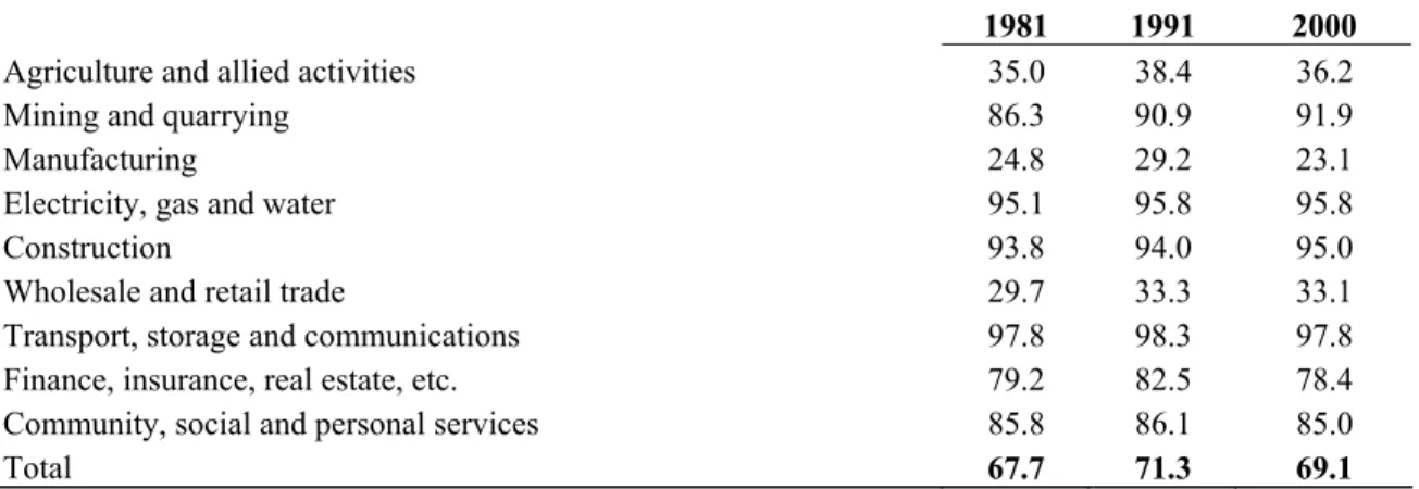
On average, there has been little change in the composition of the unorganized sector in the last decade. Agriculture and trade occupations remain nearly fully informal.

In mining and quarrying; transport, storage and communication; finance, insurance and real estate; and community, social and personal services, the informal sector accounts for

half to four-fifths of total employment. In the electricity and gas industry, almost all employment is formal, but only 7% is formal in construction and 14% in manufacturing.

From 1991 to 2000, the proportion of unorganized sector employment declined slightly in mining and quarrying, possibly reflecting increasing control of natural resources by the State. On the other hand, in construction, transport and finance the share of informal employment increased considerably, reflecting the expansion of private sector enterprises in these industries (Table 1).

The public sector accounts for almost 70% of organized employment (in 2000), a slight decline from 1991. Organized public employment is least prevalent in agriculture, manufacturing and trade (ranging from 23 to 36%). Nearly all organized employment in mining, electricity, and transport and over 80% of the total organized employment in community, social and personal services are accounted for by the public sector (Table 2).

The share of the Central government in the public sector workforce has been declining over the last two decades and the Central government employed only 17% of the total public sector workforce in 2000. State governments and quasi government units, each of which provides employment to third of public sector employees, grew rapidly in the 1980s and continued to grow (at a much slower rate) in the 1990s (Table 3).

Wage Setting Policies

The government actively participates in wage setting in India. Following the recommendations of the 1948 Committee on Fair Wages, the government started providing guidelines for wage structures. These guidelines defined living wage that would provide not only for physical subsistence but also for the maintenance of “health and decency and insurance against misfortunes”. In practice, these goals are reflected in the government’s setting of the minimum wage. The government set minimum-wage guidelines for the organized sector, while the 1948 Minimum Wage Act covered wage setting for the informal sector. However, evidence suggests that minimum wage was rarely enforced outside of the organized sector.

Wages of public administration employees and employees in the departmental undertakings are regulated by the Government Pay Commissions. Wages for employees in the Central government civil service have two components: basic pay and dearness

allowance (DA). The latter is meant to compensate for increases in cost of living. DA and basic pay vary by grade. Both are revised based on recommendations of pay commissions. DA is also applied to the basic pay of non-departmental public undertaking employees.

The wage determination in the public sector enterprises (companies and corporations) is governed by the Industrial Dispute Act of 1947. Workers’ unions and the management of each organization settle on wages through a collective bargaining process. Factors considered in the negotiations include: level of skill or responsibility required in each category of work, the wage scale paid in similar activities in the private sector or in other government departments, the degree of unionization in the enterprise and in the industry, the bargaining strength of the workers relative to management, and the paying capacity of the enterprise. State government non-departmental undertakings either follow their own wage standards or conform to Central government standards. In addition, the Payment of Bonus Act recommends an incentive scheme so that every employer is to be paid a minimum bonus of 8.33% of the salary or wage earned during the accounting year. Several public enterprises have also introduced productivity-linked incentive schemes. In the organized private sector, wages are set through a collective bargaining process and in some industries by industry-wide tripartite wage boards.

Many fringe benefits are available to civil service employees and employees in departmental undertakings. Central and state government employees are eligible for a number of allowances in addition to DA that could constitute up to 18% of total pay. All government civilian employees and those in public enterprises are entitled to these allowances. In addition, five major social insurance schemes complement incomes in the organized sector.

In the informal sector, the most recent policy initiative undertaken by the Central government was the enactment of the Building and Construction Workers Act, 1996, aimed at protecting the interests of workers engaged in the construction industry (Unni, 1998). However, there is no monitoring of the implementation of minimum wages in the unorganized sector and ample anecdotal evidence suggests that minimum wage is not enforced. Within the unorganized sector, the most robust relationship is between wages and productivity (Mitra 2001; Patel and M. Gandhi 1998).

3. Public and Private Wages in India (knowledge to date)

The paucity of evidence on the magnitude of the wage differentials for the Indian labor market as a whole is usually blamed on the scarcity of suitable data. Even though many agencies collect some information on employment and wages, the comparability of public and private sector wages is complicated because wage data are rarely collected in conjunction with information on the qualifications of workers. Thus, the notion of alternative wages is rarely used. Yet, some data from formal sources exist and several authors have analyzed wages and wage differentials using individual-level data. Overall, the information on the differences in wages is limited to the factory sector, to the segment of the labor market, which employs highly skilled workers, and to some geographic areas.

Data on wages from the 1997-98 Annual Survey of Industries (Central Statistical Organization, Government of India), which covers the factory sector, suggest that the public sector offers higher remuneration for workers compared to the private sector.

There are substantial variations in pay within the public sector. Workers employed in units owned by the Central government receive wages that are nearly twice as high as the sector average; followed by workers in units owned jointly in the public sector. Workers in “wholly” private enterprises appear to receive the lowest wages among all considered categories (Table 4).²

Several authors have attempted to account for differences in the human capital of workers in the public and private sectors while investigating wage differentials. Most of these studies used the survey of Degree Holders and Technical Personnel (DHTP) conducted, along with the 1981 Census of India, on behalf of the Division of Scientific and Technical Personnel of the Council for Scientific and Industrial Research. Data were collected on the basis of a 20% Census sample in 12 states and using the complete enumeration samples in other states and union territories.

2The 1999-2000 Annual Survey of Industries data on wages has not been released as yet. Various media sources state that the high differential between public and private workers in the factory sector remained. In particular “According to the Annual Survey of Industries for 1999-2000, in the top ten industrialized states, the average annual wage difference between public and private sector industrial workers varies between Rs 12,000 and Rs 90,000. Industrial workers in the public sector are earning 15 to 80% more than the wages earned by workers in the private sector… In Haryana, the wage differential is around 36%, while in Uttar Pradesh it is 45%.” by Mamata Singh at: http://www.rediff.com/money/2002/may/22psu.htm).

Duraiswamy and Duraiswamy (1995) used the DHTP data to estimate earning functions for public and private sector workers, and decompose earnings differentials into two parts – one reflecting differences in productive characteristics or “endowment” and the other reflecting differences in pay structures, or premiums, attached to particular characteristics common to both sectors (Blinder and Oxaca 1970). The authors found that wages are higher in the private sector and that about 87% of the sectoral wage difference could be attributed to the higher premium paid by the private sector, while the rest could be attributed to the superior human capital of private-sector workers. They showed that the endowments and the returns on these endowments are higher in the private sector, except for female and scheduled caste (SC) and scheduled tribe (ST) workers.

Madheswaran (1998) also applied Blinder-Oxaca (1970) decomposition to the DHTP and showed that the overall unadjusted wage differential (average public wage divided by average private wage) was 0.85, and that superior human capital endowments of workers in the private sector account for 29% of this difference.³ For females, however, especially those from SC and ST, public wages are higher than private wages.

Similar to Duraiswamy and Duraiswamy (1995), Madheswaran found that returns to productive characteristics were higher in the private sector, except for female and SC/ST workers.

Using DHTP data, Lakshmanasamy and Ramasamy (1999) model workers’

choice of sector of employment with the expected sectoral wage differential as one of their explanatory variables. Madheswaran and Shroff (2000) used a sub-sample of science graduates, around 40% of the DHTP sample, to examine public-private wage differentials among men and women. These authors also found that, on average, wages in the private sector are higher than the private sector wages.

4. Data, Definitions and Stylized facts

Data for this study come from Round 50 and Round 55 of the all-India household survey collected routinely by the National Sampling Survey Organization (NSSO), Department of Statistics and Program Implementation, Government of India. Both Round 50 and Round 55 are so-called quinquenial surveys, which include a Consumption Survey (CS)

3The difference with the Duraiswamy and Duraiswamy (1995) study is possibly a different specification of the earning functions.

and an Employment and Unemployment Survey (EUS). Round 50 was carried out from July 1993 to June 1994 and EUS covered a sample of approximately 565,000 individuals (115,400 households); Round 55 took place between July 1999 and June 2000 and EUS covered about 595,500 individuals in 120,400 households. This study uses the 1993-94 and 1999-00 EUSs.⁴

EUS instruments are broadly similar for the 50^th and 55^th rounds, and gather information about demographic characteristics of household members, weekly time disposition, and their main and secondary job activities. Twenty principle job activities are defined consistently across the two survey rounds for all household members. These activities distinguish all respondents and their family members as: self-employed, regular salaried worker, casual wage laborer, unemployed, or domestic worker, among others.

Employed respondents are asked a wide-range of questions about their main job (industry, occupation, type and size of enterprise, etc.), as well as about their subsidiary economic activities. Only those who work at regular salaried jobs or as casual laborers are asked to report their weekly wages (both cash and in-kind).⁵

The sample selected for this analysis consists of those employed and working for wages (leaving out those who are self-employed and work for profit and unpaid family workers), see Figure 1. We define total wages as the sum of weekly cash and in-kind wages from the principal activity. We adjust nominal wages for differences in price levels across urban and rural areas and states, and for temporal changes in price levels between 1993 and 1999, using the indexes developed by Deaton and Tarozzi (2000). Thus, all wages in the paper are expressed in terms of the 1999 average of India’s rural prices.

Workers engaged in salaried occupations were asked about the type of enterprise where they carried out their main work activity. In the 50^th round, all salaried workers were asked to choose from three categories: public, private, or semipublic, and we

4These cross-sectional surveys use a two-stage stratified sampling design, and are representative of the national, state, and so-called “NSS region” level. The first-stage sampling units (FSUs) are census villages in the rural areas, and the NSS Urban Frame Survey (UFS) are blocks in the urban areas. The second stage units are the households in both urban and rural sectors. For more information on the survey and sample design see, e.g., NSSO, Ministry of Planning (1994, 2000).

5 In the 50^th round, the sector of employment – public or private – is defined only for those engaged in regular salaried/wage work (in all industrial activities), while in the 55^th round, it is defined for those who are employed in non-agricultural activities. In both rounds, wages are defined for everyone who reported being employed. In order to maintain consistency and comparability across the two rounds, the classification of the sector of employment was defined only for those with regular salaried/wage employment in non-agricultural industries. We also excluded casual workers in public works as well as individuals who were sick or did not work for other reasons.

combined public and semipublic workers in one group. In the 55^th round, workers were presented with eight categories: proprietary male, proprietary female, proprietary partnership with members of the same household, proprietary partnership with members of a different household, public sector, semi-public sector, and cooperative society or an enterprise covered by the Annual Survey of Industries. The last category (5% of the sample of wage earners) could include enterprises from both public and private sectors.

In addition, nine percent of the sample of wage earners had their answers coded as “0”

corresponding to “not recorded”. For the respondents with unidentified enterprise type we impute the value for sector-of-employment indicator, based on existing auxiliary information. We considered the 3-digit industry code in NSS 55^th round and examined the public/private composition in the same industry code in NSS 50^th Round. If employment within an industry code exceeded 95% public in 50^th Round, we assigned the same indicator for the missing values in 55^th Round. We applied an additional filter for assigning an individual to the public sector: whether that individual is covered by Government Provident Fund (GPF) or not. Because certain industries are reserved for public activities only and GPF covers only public sector workers, we believe, we were able to predict quite accurately the public/private status for the workers with this category missing⁶.

The sample for the present analysis consists of 82,283 individuals in 1994-94 and 86,616 individuals in 1999-2000. Among those, in 1993-94, 16% worked in formal public, 14% in formal private and 66% in informal casual sectors. The corresponding numbers for 1999-00 are 14%, 16%, and 66%. In both rounds, the “don’t know” response about the sector of employment among workers in the formal sector averages between 2 and 4% of the sample.

Characteristics of the workforce in these sectors varied substantially. In 1999-00, slightly less than 30% of the total selected sample resided in urban areas, while more than 60% of all public workers and about 70% of all formal private workers did so. Males represented about 85% in the public and formal private sectors and 70% in the salaried

6 Changes in the definitions of the public/private categories between the 50th and 55th rounds of the EUS complicate the comparability of 1993 and 1999 employment data. We examined whether the implemented imputations resulted in biasing for or against our main conclusions (i.e. whether the estimated wage differential was smaller or larger with imputation than it was without). It turns out that the public/private differential is lower with imputation, indicating that imputation biases against our results. The results for a sub-sample that excludes individuals with unidentified enterprise type are available from the authors upon request.

casual occupations. The main difference in the industrial structure of the public and formal private sectors was that more than 80% of all public sector workers were in service occupations, compared to 53% in the formal private sector. Industrial workers make up another 37% of the formal private sector. The majority of casual workers are in agricultural occupations.

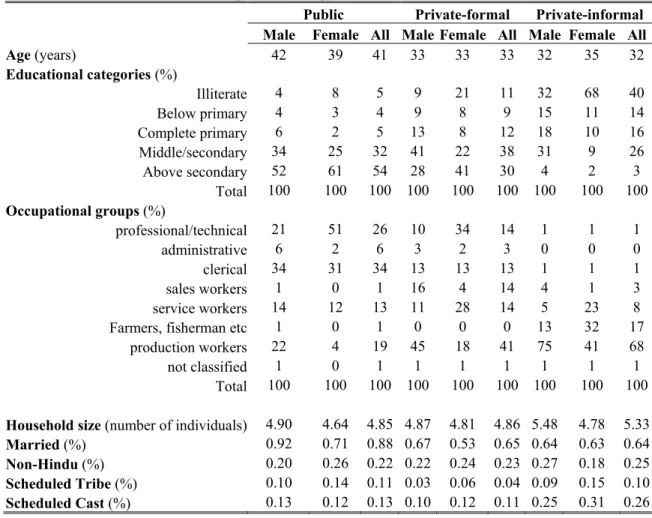
In the urban market (Table 5), public workers are considerably older than workers in the formal private and casual occupations. The average age in the urban public sector is 41, while it is 33 and 32 in the urban private and casual sectors, respectively. Both in the public and formal private sectors, the majority of workers have a middle school education or above. In the public sector, however, the proportion of workers with education above the secondary level is almost twice as high as the proportion in the formal private sector. The educational structure of men and women tends to be quite similar in the public sector. In the formal private sector a higher proportion of women are both illiterate and recipients of a secondary-school education compared to men. In the casual sector, almost 40% of workers are illiterate, but a large proportion of them are also recipients of middle- and secondary-school education. In terms of occupational distribution, the highest proportion of all public workers in urban areas have clerical occupations (34%), while the highest proportion in the private sector have production- related jobs (41%). Professional and technical occupations are most prevalent in the public sector. Public and formal private workers tend to have smaller household sizes as compared to casual workers; public workers are also more likely to be married than those in the other two sectors. The proportion of ST workers in public and casual occupations are the same, but STs are underrepresented in the formal private sector. SC workers are underrepresented both in the public and formal private sectors relative to casual laborers.

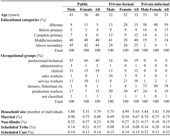
In the rural market (Table 6) public sector workers tend to be older than workers in the formal and informal private sectors. Similar to the patterns in the urban market, the majority of workers in the public and formal private sectors have attained at least a middle school education. The proportion of workers with education above the secondary level is almost twice as high in the public sector as in the private sector. The difference in education attainment among men and women is lowest in the public sector, while formal private sector employs men and women with different levels of education. In contrast to the urban market, where about a quarter of all workers in casual occupations have a

middle-secondary- or secondary-level education, only 14% of rural casual workers do, and 60% of them are illiterate. In terms of occupational distribution, the single most common type of employee in the rural public sector is the professional and technical worker, whereas the majority of formal private sector workers engage in production work (the latter pattern is similar to that in the urban market). Women who are employed in the public or formal private sector are more likely than men to be professional/technical workers. Clerical work is the second largest form of employment in both the public and private sectors. Public workers tend to live in the larger households, and are more likely to be married and non-Hindu. In rural areas, the ST are over-represented in public occupations compared to the formal private ones. The SC are underrepresented in formal private occupations.

5. Theoretical Model and Estimation Methodology

The unadjusted wage differential could be calculated as a ratio of average wages of workers employed in different sectors, but in order to make inferences about differences in wages of workers with similar human capital characteristics (but working in different sectors) one needs to estimate the models of individual’s earning function and sectoral choice. There are several commonly used approaches to estimation of the inter-sectoral wage differential. However, there is no consensus among the economists about what method is preferable. Each method relies on a different set of assumptions about the underlying processes of determination of wages and sector choice, and the choice of the methodology rests on one’s belief about how realistic these assumptions are. Different methods highlight various aspects of the underlying processes of determining the wage differential, and thus could provide answers to different but relevant questions. It is customary to apply a set of techniques to test the robustness of the estimation results – the practice we employ in this study.

We start with reporting the ratios of the “raw” average wage in public, private- formal and private informal sectors across occupation, age, education and “skill” groups.

We then move to presenting the simple non-parametric estimation of wage differentials by employing the Ordinary Least Square (OLS) regression relating wages of workers employed in three sectors to their productive and human capital characteristics.

Compared to simple means, application of the OLS allows adjusting for the difference in human capital characteristics between workers in public and private sectors. Next, we employ a sector selection bias correction (SBC) method which models wage setting mechanisms in each sector as a function of both observable and unobservable characteristics of workers and employers. Finally, we use a non-parametric technique called Propensity Score Matching (PSM)⁷.

Our empirical analysis is motivated by a model of an individual’s choice of sector of employment that is commonly presented in terms of utility maximization and human capital. Suppose the marginal productivity of a worker is determined by her/his human capital and personal characteristics. To choose between the sectors, an individual compares expected net benefits in each sector and selects the job that best rewards his individual set of characteristics. Once an individual decides on the sector in which to seek employment, she/he enters the pool of applicants from which employers select. The probability of being selected in a particular sector depends on the individual’s characteristics (observed and unobserved) as well as on characteristics of the employer.

The observed individual outcome is a combination of preferences and rationing. First, an individual seeks to join, for example, the public sector if the expected benefits in that sector exceed her/his expected benefits in the private sector and in the informal sector.

Second, he is selected by the employer and actually hired into the sector.

To formalize this approach, let Vis be the indirect utility function of individual i employed in sector s, we assume that Vis can be linearly characterized as:

(1) Vis=Ziγ+ηis, s=1,…,3

where Zi is a vector of characteristics of the respondent i, γ is a vector of parameters, s is a categorical variable describing sector choice, and ηi•’s are IID error terms. The individual is employed in sector s if:

(2) Vis >max(Vij) j≠s, s=1,…,3

The wage in a particular sector is observed only if the sector is chosen:

(3) Wis=βsXi +µis, s=1,…,3 if Vis >max(Vij) j≠s

7We know of only one attempt to use PSM for measuring inter-sectoral wage differential, see Bales and Rama (2002). While in Bales and Rama the matching is based on the probability to be employed in the public sector, this study matches workers based on their predicted probabilities to work in each of three sectors.

where Xi is a vector of explanatory variables that determine the wage level, β is a vector of parameters, and µi•‘s are the normally distributed error terms with mean 0 and variance σ².

Estimation of equation (3) for three sectors (public, private formal and private informal) by the OLS allows inferring about the returns to characteristics in each sector i.e., the sector-specific wage structure. Once estimates of these returns are obtained, one can predict for the public sector workers expected wages in the own and the alternative sector and then derive the corresponding wage differential.

If the error terms in equations (1) and (3) are independent, the probability that the person is employed in sector s could be estimated by the standard multinomial logit or probit and the earning function (3) could be specified in the traditional human capital form (Mincer 1974). In case of a multinomial logit specification the probability to be employed in sector s could be estimated as:

(4) ^{> =} ∑j ij j j^≠s s is s

s

is Z

Z Z

P exp( )

) ) exp(

( γ

η γ

γ s=1,…,3

Sector selection bias correction (SBC) method

However, some unobserved individual characteristics could affect both the choice of the sector of employment and the wages that the individual earns in the chosen sector. For example, an individual with high entrepreneurial abilities might choose to work in the private sector. These abilities could also allow him to earn higher wages in that sector in comparison with the average worker who enters the labor market. Employment in the public sector could depend, for example, on personal connections, which might also influence individual earnings. Thus, error terms in equations (1) and (3) could be correlated. If error terms µ’s and η’s are not independent, the explanatory variables Xi

and µ’s may show some correlation, and the OLS estimation of the wage equation (3) could be biased.

To obtain unbiased and consistent estimates of the parameters in the system of equations (3) and (4) under an assumption of joint dependence of the error terms in these equations, it is common to employ a two-stage selection bias correction proposed by

Heckman (1978). The modification proposed by Bourguignon, Fournier and Gurgand (2002) extends this approach to models with more than two sectors.

In terms of empirical strategy, this leads to a two-stage estimation procedure. On the first stage, we estimate the sector of employment choice model (4) and generate the selection term (similar to Mill’s ratio in standard Heckman’s type estimation) for every alternative j:

(5) ( ),

) 1 ) (

( _s

j

s s

s j j

j

j m P

P P P

m ∑

≠ −

+

=ρ ρ

λ

where ρj is the correlation between ηij and µij, and Ps is the probability that category s is chosen and given by equation (4). On the second stage, we estimate equations (3) with the choice-specific λj included together with other explanatory variables. This leads to the following specification:

(6) ln(Wis)=βsXi +σsλs+vis, s=1,…,3 where νis is IID error terms uncorrelated with η’s.

The system of equations (3) and (4) is identified by non-linearities even if variables in X and Z overlap completely under the specific distributional assumptions on the error terms. In order to improve the efficiency of estimates and computational stability we impose stronger identification restrictions on the model. Our specification includes some variables that influence the selection into the sector, but do not influence the individual wage. We use four variables: household’s land ownership and size, and individual’s recent migration status and marital status. These variables may account for the importance of a secure job and associated benefits. We test the assumption that these variables affect the sectoral choice decision but do not influence wages conditional on the sector choice.

Once unbiased estimates of these returns are obtained, we can predict expected wages in each sector and derive the corresponding wage differentials. We calculate the conditional wage differential based on conditional wages in each sector. The conditional wage measures what would be the wage of public sector workers if they faced the wage

structure prevailing in the private (formal or informal) sector. It is defined only for public sector workers in the sample and presented in equation (7) ⁸.

(7) , 1,...3

exp 2 )

| ) (exp(ln(

2

 =











 + +

=

=

=E W s j X j

W_ij^C _{ij j i j j} σ^j

λ σ β

The reliability of the estimated results strongly depends on the validity of the assumption about the joint normality of the error terms in equations (3) and (4). If the joint distribution of the error terms in the system (1-3) is non-normal, the estimated coefficients of wage equations could be severely biased. To overcome this potential problem we apply an alternative method known as Propensity Score Matching (PSM) method, following Rubin (1974) and Rubin and Thomas (1996).

Propensity Score Matching method (PSM)

The PSM balances the distributions of observed covariates between a treatment group and a control group based on similarity of their predicted probabilities of being employed in the public or private sectors (their “propensity scores”). The propensity score is a constructed indicator that combines information about individual’s characteristics into an index normalized to the scale between 0 and 1. This method does not require any parametric assumptions linking sectoral choice to wages, and thus allows estimation of mean impacts without arbitrary assumptions about functional forms and error distributions. Rosenbaum and Rubin (1983) show that an exact matching by propensity scores implies that workers from two sectors have the same distribution of covariates.

When the relevant differences between any two workers are captured in the observable covariates, PSM yields an unbiased estimate of the wage differential for the considered group.

The standard PSM approach usually compares outcomes between two groups (the public and private sectors in our case). The propensity score then measures the probability that an individual work in the public sector as a function of that individual’s

8Some studies also consider an unconditional wage differential. Unconditional wage is defined as 3

,...

1 2 ,

exp )) (exp(ln(

2

 =











 +

=

=E W X j

W_ij^O _{ij j i} σ ^j

β ^. The unconditional wage could be interpreted as wage that an “average” individual would face if he joins either sector by some random assignment. The unconditional wage is defined for all workers (in public, private and informal sectors) in the sample. We do not present the unconditional differential in this paper.

observed characteristics. In case of employment choice in India, some complexity is added by the fact that there are three outcomes: an individual could work in the public, private formal or private informal sectors. In this study, we do pair-wise comparisons of wages between sectors, and utilize additional information on the probability to be employed in all three sectors to improve the efficiency of our estimates. The literature on evaluation models with multiple treatments is rather recent (e.g., Lechner 2002; Imbens 1999) and we follow the methodology suggested in Blandel et al (2001).

In order to take into account the fact that the workers could be employed in one of three sectors we use propensity score matching based on two dimensions: the probability to be employed in the public P1i=P(s=1|xi) and the probability to be employed in the private sector P2i=P(s=2|xi). We use the nearest neighbor matching with replacement where each public sector worker is paired with the worker from the private formal and informal sectors based on the score that minimizes the Euclidean distance with respect to the two propensity scores conditional on two maximum distance restrictions and identification conditions.

To measure the wage differential between the public and, for example, private sector, we use the standard estimator of the average treatment on the treated defined as:

E(w1 – w2| s=1). This allows us to estimate the mean effect of being employed in the public sector relative to the private sector. We also define the average effect conditional on some set of characteristics as: E(w1 – w2| s=1,x).

For some individuals in our sample we may not find proper matches. This is the problem of no common support region. If there are regions in the data where the support of x does not overlap for the public and private sector workers, there may be a fraction of public sector workers for whom no match could be found in the data. According to various studies by Heckman, Ichimura and Todd (1997, 1998), matching on the no common support region is the primary cause of a bias in a matching estimator. In this study we calculate wage differentials only for the workers on a common support.

6. Findings: Wage Differential in 1999-00

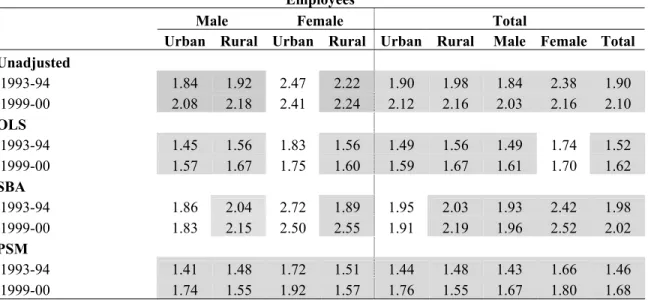
The average weekly wage among all salaried workers in India, expressed in terms of 1999 rural prices, was Rs.432 (Table 7). Public sector workers earned an average of

Rs.1,240 per week, followed by formal private sector workers at Rs.590, and informal casual laborers at only Rs.224 per week.⁹ This salary range translates into a 2.1 unadjusted wage differential between the public and formal private sectors and a 3.81 differential between public and casual wages.¹⁰

In 1999, the public-private wage differentials were higher in rural as compared to urban areas, and larger among women than among men, whether rural or urban. Of the four groups of workers distinguished by gender and type of residence (urban males, rural males, urban females, rural females) the public-private differential was largest for urban females, followed in order by rural females and rural and urban males¹¹.

Differences in earnings can vary depending on the level of experience, education and skill of a worker, and on the demand and supply conditions for various type of labor.

Table 8 presents wage differentials between the public and private formal sectors, by age, education level, and occupation. Several patterns emerge.

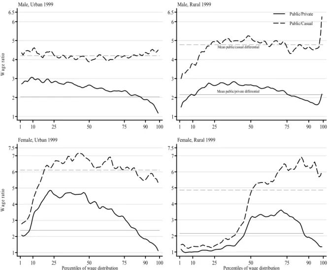
The higher differential is observed among the workers with lowers skills (i.e., in sales, services, production occupations) as compared to more high-skilled workers (professional and administrative occupations). The public-private wage differential among urban and rural males is higher for the younger group of workers. In urban areas, the wage differential generally decreases as education increases for both men and women. In rural areas, the differential seems to be largest at the complete primary school levels for both men and women.

Figure 2 plots the wage differentials at every percentile of the distribution for four groups of workers. Similar to the patterns observed above, the differential tends to be larger at the lower percentiles (the low-skilled workers) and smaller for the highly skilled workers. These patterns roughly hold for men and women, and in urban and rural areas, but are especially pronounced for males in urban areas (a group that constitutes 50% of the public sector workforce).

9All–India average rural per capita monthly poverty line was set at Rs. 328 in 1999-00.

10 In this paper we define the differential as a ratio of average public and private-formal (public and private- casual) wages: wage differential =(averageW_public)/(average W_private). We choose to define the differential as a ratio because most of the existing literature on wage differentials in India uses this measure.

11 In this paper we report wage differentials between the public and formal-private sector workers. Results pertaining to the differences between wages of public and informal-private sector workers are presented in the longer version of the paper (which was prepared as a background paper for “India – Sustaining Reform, Reducing Poverty”, a World Bank Development Policy Review released in July 2003). The longer version is available from the authors upon request.

Ordinary Least Squares (OLS) estimates

Table 9 presents OLS-based wage differentials between the public and private sectors, by age, education level, and occupation for four groups of workers distinguished by gender and type of residence. Similar to the patterns of unadjusted differentials, wages of public sector workers are higher than their wages would have been, had they been employed in the private sector for nearly all groups of workers. Overall, the wage advantage of public sector workers represents 62%; it is 57% among urban men and it reaches 75% among urban females. Wage differential is higher in rural, as compared to urban, areas.

With respect to differences across occupational groups, among urban men, the highest differential is registered among sales workers who receive a 75% wage premium.

Professional and technical employees and men working in administrative occupations enjoy a 50% wage advantage. Among rural men, professional and technical public sector employees receive wages twice as high as they would have had they been in the private sector, and have the highest wage advantage across all occupational categories. Among rural women, the highest public-private wage differential of 116% is observed in sales occupations. Professional and technical female employees in urban areas earn wages that are 109% higher than the wages in the same occupation in the private sector. Alternative wages of public sector workers would have been higher only for women working in some occupational categories (administrative and sales occupations).

The wage differential of young and pre-retirement-age workers is lower than the wage differential of workers in the twenty-six to forty-five age range, on average. In urban areas, wage differential declines with age from about 60% for the younger group to 52% for male workers forty-six to fifty-five years old. In rural areas, the wage differential is the highest for the twenty-six to thirty-five age group where it reaches 77%. The wage differential among young urban women is 54%; it rises to 86% for women twenty-six to forty-five age range, and drops for older women.

While the overall wage differential tends to be higher among workers with a middle-school diploma as compared to workers with less and more education, for urban males the public-private wage ratio is higher for workers with a lower level of education.

For example, the ratio of public to private sector wages is equal to 1.7 for illiterate workers and 1.5 for employees with a university degree or higher. In rural areas,

however, the highest wage differential of 76% is registered among university-educated workers, while it is only 50% among illiterate rural males. Wage differentials among illiterate urban female workers is high (about 93%), and it is similar to that of women with secondary-education levels. The lowest wage differential is registered among urban women with a middle-school diploma.

Estimates with sector selection bias correction (SBC)

As Table 10 shows, on average, and for nearly all groups, the conditional public-private wage differentials estimated by the SBC is higher than the corresponding wage differential estimated by the OLS. Since the conditional differential measures the ratio of current (in public sector) to potential (in private sector) wages of public sector employees, taking into account their self-selection, this possibly reflects the self-selection of individuals in the sector that offered them a higher comparative wage advantage.

Similar to the OLS estimates, the selection bias corrected wage advantage is higher in rural than urban areas, and it is higher among women than men. Public sector wages are about 83% higher than alternative wages in the private sector for urban male employees; the ratio of public-to-private wages is even higher for rural males (2.15), and it is as high as 2.5 for female workers. Patterns of wage differential with respect to occupation are roughly similar to those estimated by OLS regressions. For urban males, the highest wage differential of 107% is registered among sales workers, followed by the differential of 92% among production workers. The wage differential among urban men in professional/technical, administrative, and clerical and service occupations ranges from 70 to 80%. In rural areas, male public sector workers in professional/technical, administrative, and production occupations enjoy wages that are more than twice as high as they would have been in the private sector. The wage advantage of rural male employees in clerical, sales, and service occupations is about 90%.

The conditional wage differential among women in service occupations is very high, reaching 289%. The private sector wage advantage of women employed in administrative and sales occupations is also higher than those of men in the same occupations. Younger men in the public sector enjoy a higher wage advantage as compared to older men. The ratio of public to private wages is close to 2.0 for male

workers in the eighteen to twenty-five age group, and it declines to about 1.9 for the workers of pre-retirement age. Middle-aged women both in urban and rural areas tend to have a higher wage advantage as compared to their younger and older counterparts.

Patterns of wage differential with respect to education level are similar to the ones estimated by the OLS. The wage differential is higher among illiterate urban male workers as compared to urban men with higher educational attainments. Among rural men, the wage differential ranges from 110% for the illiterate to 122% for workers with university or higher education. The ratio of public-to-private wages is highest among illiterate urban women, followed by urban women with complete primary and above- secondary education.

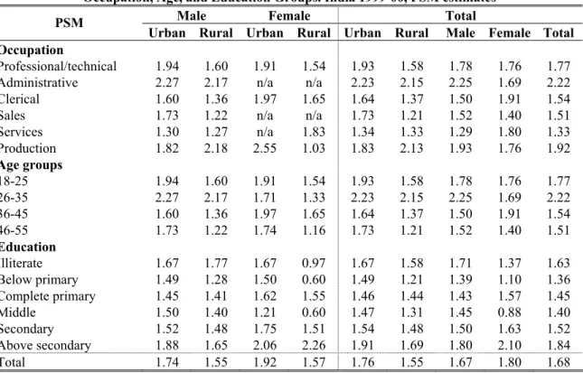
Propensity Score Method (PSM) estimates

Wage differentials presented in Table 11 measure the ratio of wages for a sample of public sector workers for whom we were able to find appropriate matches, i.e., workers with identical observable characteristic, but employed in the formal private sector.

The magnitude of the PSM-estimated wage differential falls between the OLS and selection bias-corrected wage differentials discussed above. As Table 11 shows, on average, the wage advantage of public sector workers over similar workers in the private sector appears to be 68%. While patterns of wage differentials with respect to occupation, age, and education are quite similar across OLS and SBC methods, PSM estimates are somewhat different. For example, workers in administrative occupations (high-skilled workers) seem to enjoy the highest wage advantage of all occupational categories; wage differentials seems to increase with age; and the overall differential in rural areas seems to be lower than in urban areas. Also, the divergence in patterns of wage differentials between the OLS and SBC estimates on one hand, and the PSM estimates on the other, is greater for women than for men. Notwithstanding these differences, that could possibly be explained by the fact that PSM uses a different sample of working individuals, the magnitudes of the wage differentials are quite similar across all three methods.

Changes in wage differential between 1993-94 and 1999-00

In 1995 the Fifth Pay Commission recommended a 30% increase in the real base pay of Central government civil servants. The pay increase recommendations were extended by the states to their employees, with these increases being implemented over the late 1990s—early 2000s. Recommendations of the Fifth Pay Commission also included decompression of the wage structure through a number of upward wage adjustments for highly skilled employees. The wages of workers in the formal private and casual labor markets also changed, following the improvements in their productivity and the changes in demand and supply conditions.

Overall, real wages grew by 29% between 1993-94 and 1999-00. Urban wages grew faster than rural wages, with the wages of urban women significantly outpacing the increase in wages of urban men.¹² Average wages in the public sector increased by 44%, in the private sector by 35% and in the informal-casual sector by 20%. The average wages of all four groups of workers in the public sector grew roughly at the same pace, but in the formal private and casual sectors they grew at very different rates. Clearly, private wages are considerably more responsive to the changes in demand for and supply of skills. In the private sector, urban females experienced the highest growth in average wages.

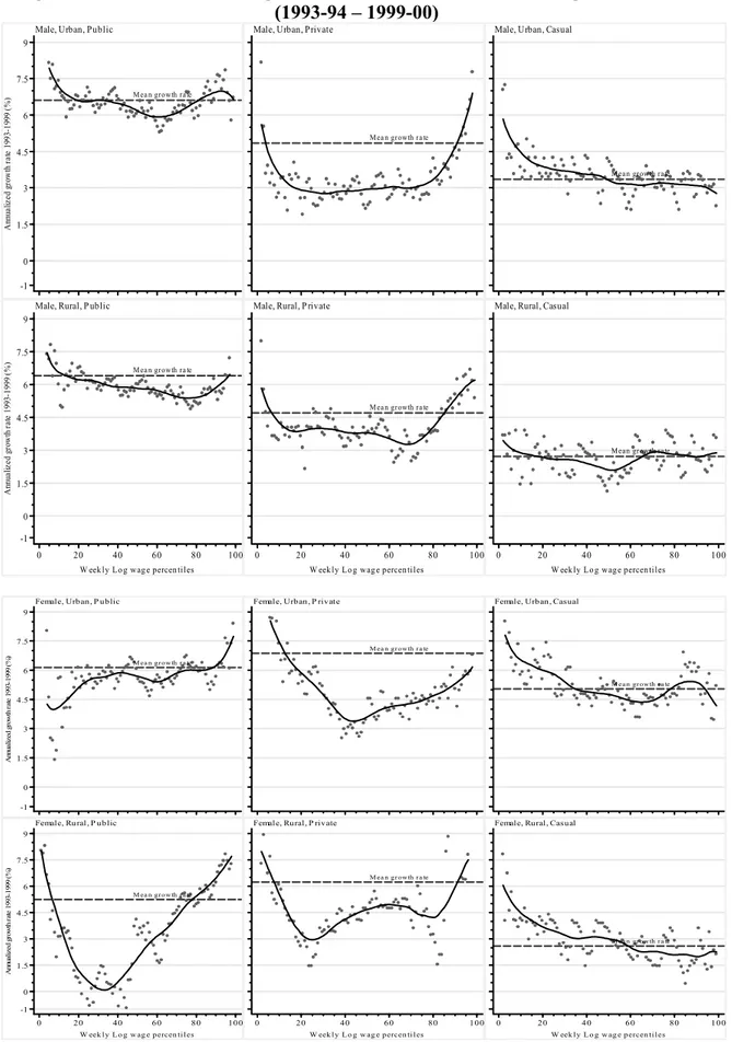
In terms of the patterns of wage increases (Figure 3), wages of low-skilled public sector workers (those with wages below the 20^th percentile) grew faster than wages of other workers both in urban and rural areas. The wages of highly skilled public workers (those above the 80^th percentile) increased faster than average wages only in urban areas.

In the formal private sector, the growth rate in wages of highly skilled workers (75^th percentile and above) was higher than the growth rate in the wages of the other workers.

In the private-informal (casual) sector, the wages of low-skilled workers in urban areas grew faster than the mean growth rate, while casual wages in rural areas increased quite uniformly across percentiles of the distribution. For female workers, the patterns of wage growth in the public sector were similar to those of males, but in the private sector there was less evidence of growth in high wages, and more growth in low wages. Growth in low wages in the casual sector was evident in both urban and rural areas.

12Ranasinghe (2004) analyzes the changes gender wage gap in urban India between 1995 and 2000.