4 Basic Concepts of Mathematical

(1)

Logic and Games WS 2015/2016

Prof. Dr. Erich Grädel

Notes and Revisions by Matthias Voit

Mathematische Grundlagen der Informatik RWTH Aachen

(2)

c b n d

This work is licensed under:

http://creativecommons.org/licenses/by-nc-nd/3.0/de/

Dieses Werk ist lizenziert unter:

http://creativecommons.org/licenses/by-nc-nd/3.0/de/

http://www.logic.rwth-aachen.de

4 Basic Concepts of Mathematical

Game Theory

Up to now we considered finite or infinite games

• with two players,

• played on finite or infinite graphs,

• with perfect information (the players know the whole game, the history of the play and the actual position),

• with qualitative (win or loss) winning conditions (zero-sum games),

• withω-regular winning conditions (or Borel winning conditions) specified in a suitable logic or by automata, and

• with asynchronous interaction (turn-based games).

Those games are used for verification or to evaluate logic formulae.

In this section we move to concurrent multi-player games in which players get real-valuedpayoffs. The games will still have perfect information and additionally throughout this chapter we assume that the set of possible plays isfinite, so there exist only finitely many strategies for each of the players.

4.1 Games in Strategic Form

Definition 4.1. A game in strategic formis described by a tupleΓ = (N,(Si)_i∈N,(pi)_i∈N)where

•N={1, . . . ,n}is a finite set of players

•S_iis a set ofstrategiesfor Playeri

•p_i:S→^Ris apayoff functionfor Playeri

andS:=S1× · · · ×Snis the set ofstrategy profiles.Γis called azero-sum gameif∑i∈Np_i(s) =0 for alls∈S.

(4)

4 Basic Concepts of Mathematical Game Theory

The numberpi(s1, . . . ,sn)is called thevalueorutilityof the strategy profile(s₁, . . . ,sn)for Playeri. The intuition for zero-sum games is that the game is a closed system.

Many important notions can best be explained by two-player games, but are defined for arbitrary multi-player games.

In the sequel, we will use the following notation: LetΓbe a game.

ThenS_−i:= S1× · · · ×S_i−1×S_i+1× · · · ×Sn is the set of all strategy profiles for the players excepti. Fors∈ Siands−i ∈S−i,(s,s−i)is the strategy profile where Playerichooses the strategysand the other players chooses_−i.

Definition 4.2. Lets,s^′∈S_i. Thens dominates s^′if

• for alls_−i∈S_−iwe havep_i(s,s_−i)≥p_i(s^′,s_−i), and

• there existss−i∈S−isuch thatpi(s,s−i)>pi(s^′,s−i).

A strategysisdominantif it dominates every other strategy of the player.

Definition 4.3. Anequilibrium in dominant strategiesis a strategy profile (s₁, . . . ,sn)∈Ssuch that alls_iare dominant strategies.

Definition 4.4. A strategy s ∈ S_i is a best response to s_−i ∈ S_−i if pi(s,s−i)≥pi(s^′,s−i)for alls^′∈Si.

Obviously, a dominant strategy is a best response to all strategy profiles of the other players.

Example4.5. The Prisoner’s Dilemma.

Two suspects are arrested, but there is insufficient evidence for a conviction. Both prisoners are questioned separately, and are offered the same deal: if one testifies for the prosecution against the other and the other remains silent, the betrayer goes free and the silent accomplice receives the full 10-year sentence. If both stay silent, both prisoners are sentenced to only one year in jail for a minor charge. If both betray each other, each receives a five-year sentence. So this dilemma poses the question: How should the prisoners act?

stay silent betray stay silent (−1,−1) (−10, 0)

betray (0,−10) (−5,−5)

4.2 Nash equilibria An entry(a,b)at positioni,jof the matrix means that if profile(i,j)is chosen, Player 1 (who chooses the rows) receives payoffaand Player 2 (who chooses the columns) receives payoffb.

Betraying is a dominant strategy for every player, call this strategy b. Therefore,(b,b)is an equilibrium in dominant strategies. Problem:

The payoff(−5,−5)of the dominant equilibrium is not optimal.

The Prisoner’s Dilemma is an important metaphor for many decision situations, and there exists extensive literature concerned with the problem. Especially interesting is the situation, where the Prisoner’s Dilemma is played repeatedly, possibly infinitely often.

Example4.6.Battle of the sexes.

meat fish red wine (2, 1) (0, 0) white wine (0, 0) (1, 2)

There are no dominant strategies, and thus there is no dominant equilibrium. The pairs(red wine, meat)and(white wine, fish)are distin- guished since every player plays with a best response against the strategy of the other player: No player would change his or her strategy unilaterally.

4.2 Nash equilibria

Definition 4.7.A strategy profiles= (s1, . . . ,sn)∈Sis aNash equilib- riuminΓif for alli∈Nand all strategiess^′_i∈Si

p_i(s_i,s_−i

| {z }

s

)≥p_i(s^′,s_−i).

Thus, in a Nash equilibrium, every player plays with a best response to the profile of his opponents, and thus has no incentive to deviate unilaterally to a different strategy. Is there a Nash equilibrium in every game? The following example shows that this is not always the case, at least not in pure strategies.

(5)

Example4.8. Rock, paper, scissors.

rock scissors paper rock (0, 0) (1,−1) (−1, 1) scissors (−1, 1) (0, 0) (1,−1) paper (1,−1) (−1, 1) (0, 0)

There are no dominant strategies and no Nash equilibria: For every pair (f,g)of strategies one of the players can change to a better strategy.

Note that this game is a zero-sum game.

Although there are no Nash equilibria in pure strategies in rock, paper, scissors, there is of course an obvious good method to play this game: Randomly pick one of the three actions with equal probability.

This observation leads us to the notion of mixed strategies, where the players are allowed to randomise over strategies.

Definition 4.9. Amixed strategyof PlayeriinΓis a probability distribu- tionµ_i:Si→[0, 1]onSi(so that∑s∈Siµ(s) =1).

∆(Si) denotes the set of probability distributions on Si. ∆(S) :=

∆(S₁)× · · · ×∆(Sn)is the set of all strategy profiles in mixed strategies.

The expected payoff ispb_i:∆(S)→^R,

pb_i(µ1, . . . ,µn) =

∑

(s1,...,sn)∈S

∏

j∈N

µ_j(s_j)

!

·p_i(s1, . . . ,sn)

For every gameΓ= (N,(S_i)_i∈N,(p_i)_i∈N)we define themixed expansion bΓ= (N,(∆(Si))_i∈N,(p_bi)_i∈N).

Definition 4.10. ANash equilibrium ofΓin mixed strategies is a Nash equilibrium inbΓ, i.e. a Nash equilibrium inΓin mixed strategies is a mixed strategy profileµ = (µ₁, . . . ,µ_n)∈∆(S)such that, for every playeriand everyµ^′_i∈∆(S),pb_i(µ_i,µ_−i)≥pb_i(µ^′_i,µ_−i).

Nash equilibria (in mixed strategies) provide the arguably most important solution concept in classical game theory (although, as we shall point out later, this concept is not without problems). An important

4.2 Nash equilibria reason for the success of Nash equilibrium as a solution concept is the fact that every finite game has one. To prove this, we shall use a well- known classical fixed-point theorem.

Theorem 4.11(Brouwer’s Fixed-Point Theorem).LetX⊆^Rⁿbe compact (i.e., closed and bounded) and convex. Then every continuous function

f:X→Xhas a fixed point.

We do not prove this here but remark that, interestingly, the Brouwer Fixed-Point Theorem can itself be proved via a game-theoretic result, namely the determinacy of HEX.

Theorem 4.12(Nash).Every finite gameΓin strategic form has at least one Nash equilibrium in mixed strategies.

Proof. LetΓ = (N,(S_i)_i∈N,(p_i)_i∈N). Every mixed strategy of Playeri is a tuple µ_i = (µ_i,s)_s∈S_i ∈ [0, 1]^|Sⁱ^| such that∑s∈Siµ_i,s = 1. Thus,

∆(Si)⊆[0, 1]^|^Sⁱ^|is a compact and convex set, and the same applies to

∆(S) =∆(S₁)× · · · ×∆(Sn)forN={1, . . . ,n}. For everyi∈N, every pure strategys∈Siand every mixed strategy profileµ∈∆(S)let

g_i,s(µ):=max pb_i(s,µ_−i)−pb_i(µ), 0

be the gain of Playeriif he unilaterally changes from the mixed profile µto the pure strategys(only if this is reasonable).

Note that ifgi,s(µ) = 0 for alliand alls∈ Si, thenµis a Nash equilibrium. We define the function

f:∆(S)→∆(S)

µ 7→f(µ) = (ν₁, . . . ,νn)

whereνi:Si→[0, 1]is a mixed strategy defined by ν_i,s= ^µ^i,s+gi,s(µ)

1+_∑_s∈S_ig_i,s(µ)^.

For every Playeriand alls ∈ Si, µ 7→ νi,s is continuous since pbiis continuous and thus g_i,s, too. f(µ) = (ν1, . . . ,νn)is in ∆(S): Every

(6)

νi= (νi,s)_s_∈_S_iis in∆(Si)since

s∈S

∑

i

ν_i,s= ^∑^s∈Sⁱ^µ^i,s+_∑_s∈S_igi,s(µ)

1+_∑_s_∈_S_ig_i,s(µ) =¹+_∑_s∈S_igi,s(µ) 1+_∑_s_∈_S_ig_i,s(µ)=1.

By the Brouwer fixed point theoremfhas a fixed point. Thus, there is a µ∈∆(S)such that

µ_i,s= ^µ^i,s+gi,s(µ) 1+∑_s∈S_igi,s(µ) for alliand alls.

Case 1:There is a Playerisuch that∑s∈Sigi,s(µ)>0.

Multiplying both sides of the fraction above by the denominator, we get µi,s·∑s∈Sigi,s(µ) = gi,s(µ). This impliesµi,s =0 ⇔ gi,s(µ) =0, and thusg_i,s(µ)>0 for alls∈S_iwhereµ_i,s>0.

But this leads to a contradiction:gi,s(µ)>0 means that it is profitable for Playerito switch from(µ_i,µ_−i)to(s,µ_−i). This cannot be true for allswhereµ_i,s>0 since the payoff for(µ_i,µ_−i)is the mean of the payoffs(s,µ₋i)with arbitraryµi,s. However, the mean cannot be smaller than all components:

pbi(µi,µ₋i) =

∑

s∈Si

µi,s·pbi(s,µ₋i)

=

∑

s∈Si µi,s>0

µi,s·pbi(s,µ₋i)

>

∑

s∈Si µi,s>0

µ_i,s·pbi(µ_i,µ_−i)

=pbi(µ_i,µ_−i) which is a contradiction.

Case2: gi,s(µ) =0 for alliand alls∈Si, but this already means thatµ is a Nash equilibrium as stated before. q.e.d.

Thesupportof a mixed strategyµi∈∆(Si)is supp(µi) ={s∈Si: µ_i(s)>0}.

4.3 Two-person zero-sum games Theorem 4.13. Letµ^∗= (µ1, . . . ,µn)be a Nash equilibrium in mixed strategies of a gameΓ. Then for every Playeriand every pure strategy s,s^′∈supp(µ_i)

pb_i(s,µ_−i) =p_b_i(s^′,µ_−i).

Proof. Assume pbi(s,µ_−i)> pbi(s^′,µ_−i). Then Playericould achieve a higher payoff againstµ₋_iif she playedsinstead ofs^′: Define ˜µ_i∈∆(Si) as follows:

• ˜µ_i(s) =µ_i(s) +µ_i(s^′),

• ˜µ_i(s^′) =0,

• ˜µ_i(t) =µ_i(t)for allt∈Si− {s,s^′}. Then

pbi(µ˜i,µ₋i) =p_bi(µi,µ₋i) +µi(s^′)

| {z }

>0

· pbi(s,µ₋i)−pbi(s^′,µ₋i)

| {z }

>0

>p_bi(µ_i,µ_−i)

which contradicts the fact thatµis a Nash equilibrium. q.e.d.

4.3 Two-person zero-sum games

We want to apply Nash’s Theorem to two-person games. First, we note that in every gameΓ= ({0, 1},(S0,S1),(p0,p1))

f∈∆(Smax0) min

g∈∆(S1)p0(f,g)≤ min

g∈∆(S1) max

f∈∆(S0)p0(f,g).

The maximal payoff which one player can enforce cannot exceed the minimal payoff the other player has to cede. This is a special case of the general observation that for every functionf:X×Y→^R

supx inf

y h(x,y)≤inf

y sup

x h(x,y).

(For all x^′,y: h(x^′,y) ≤ sup_xh(x,y). Thus infyh(x^′,y) ≤ infysup_x h(x,y)and sup_xinfyh(x,y)≤infysup_xh(x,y).)

(7)

Remark4.14.Another well-known special case from mathematical logic is that∃x∀y Rxy|=∀y∃x Rxy.

Theorem 4.15(v. Neumann, Morgenstern).

LetΓ= ({0, 1},(S0,S1),(p,−p))be a two-person zero-sum game. For every Nash equilibrium(f^∗,g^∗)in mixed strategies

fmax∈∆(S0) min

g∈∆(S1)p(f,g) =p(f^∗,g^∗) = min

g∈∆(S1) max

f∈∆(S0)p(f,g).

In particular, all Nash equilibria have the same payoff which is called thevalueof the game. Furthermore, both players have optimal strategies to realise this value.

Proof. Since(f^∗,g^∗)is a Nash equilibrium, for allf∈∆(S0),g∈∆(S1) p(f^∗,g)≥p(f^∗,g^∗)≥p(f,g^∗).

Thus

g∈min∆(S1)p(f^∗,g) =p(f^∗,g^∗) = max

f∈∆(S1)p(f,g^∗). So

fmax∈∆(S0) min

g∈∆(S1)p(f,g)≥p(f^∗,g^∗)≥ min

g∈∆(S1) max

f∈∆(S0)p(f,g) and

fmax∈∆(S0) min

g∈∆(S1)p(f,g)≤ min

g∈∆(S1) max

f∈∆(S0)p(f,g)

imply the claim. q.e.d.

4.4 Regret minimization

To motivate the concept of regret minimization we consider

Example4.16.Traveller’s Dilemma.This is a symmetric two-player game Γ= ({1, 2},(S1,S2),(p1,p2))withS1=S2={2, . . . , 100}and

4.4 Regret minimization

p1(x,y) =











x+2 ifx<y,

y−2 ify<x, p2(x,y) =p1(y,x) x ifx=y,

The only Nash equilibrium in pure strategies is(2, 2)since for each (i,j)withi̸= jthe player that has chosen the greater number, sayi, can do better by switching toj−1, and also, for every(i,i)withi>2 each player can do better by playingi−1 (and getting the payoffi+1 then). Also most other solution concepts from game theory (such as the iterated elimination of dominated strategies discussed in the next section) suggest that the players should choose 2.

However, experiments show that people (even game theorists!) tend to select large numbers, in the range between 90 and 100; moreover they seem right to do so, since they perform much better in these experiments than those who follow what game theory proposes and select strategy 2.

The question arises whether there are alternative solution concepts that justify the choice of large strategies in the Traveller’s Dilemma, and if yes, which one. A relatively recent proposal that seems to achieve this isregret minimization. When a player uses this concept, he wants to minimize the lost payoff (which he would “regret”) due to not playing with the best response to the strategies of the other players.

This idea was formulated in the context of decision theory, concerned with the choices of individual agents rather than the interaction of different agents as in game theory. Accordingly, the payoff is determined by a binary function p : S×Z →^R, whereSis the set of strategies of the player we are considering, andZis an abstract set of possiblestates.

Before we can introduce regret minimization, we need several defi- nitions. In statez∈Z, the maximal payoff for our player is

p^∗(z):=max

s∈S p(s,z),

and if the player chooses the strategys∈S, he will miss the following payoff:

(8)

regret_p(s,z):=p^∗(z)−p(s,z).

The overall maximal regret for the strategysis maxreg_p(s):=max

z∈Zregret_p(s,z).

Now, the decision with respect to regret minimization would be:Choose s∈S such thatmaxregp(s)is minimal.

Let us reconsider Example 4.16. Since it belongs to game theory,Z is the set of strategy profiles of the other players. We claim that exactly the strategiess∈ {96, . . . , 100}minimize the maximal regret. To see this, note that for thoses, we have that maxregp(s) =3, since

• ift≤s, thenp(s,t)≥t−2 andp^∗(t)≤t+1, thus regretp(s,t) = p^∗(t)−p(s,t)≤t+1−(t−2) =3,

• ift>s, thenp(s,t) = s+2 andp^∗(t)≤101, thus regretp(s,t)≤ 101−(s+2) =99−s≤3,

and on the other hand,

• regretp(96, 100) =101−98=3,

• fors∈ {97, . . . , 100}, regretp(s, 96) =97−94=3.

Also, fors ≤ 95, we have that maxregp(s) ≥ 4, as maxregp(s) ≥ regretp(s, 100) =101−(s+2) =99−s≥4.

Consequently, regret minimization suggests a strategyswith 96≤ s≤100. We will now iterate this idea. If both players eliminate strategies which do not minimize the regret, we obtain a subgame with strategies {96, . . . , 100}. In this game, we have that

• maxregp(97) =2, since

– regretp(97, 100) =101−99=2, – regretp(97, 99) =100−99=1, – regretp(97, 98) =99−99=0, – regretp(97, 97) =98−97=1, – regretp(97, 96) =96−95=2.

• maxregp(100)≥regretp(100, 99) =100−97=3.

• maxregp(99)≥regretp(99, 98) =99−96=3.

• maxregp(98)≥regretp(98, 97) =98−95=3.

4.5 Iterated Elimination of Dominated Strategies

• maxregp(96)≥regretp(96, 100) =101−98=3.

Hence, 97 is the unique strategy which minimizes the regret in this subgame and thus is the choice of a player who assumes that his opponent wants to minimize his regret as well.

4.5 Iterated Elimination of Dominated Strategies

Besides Nash equilibria and (iterated) regret minimization, the iterated elimination of dominated strategies is a promising solution concept for strategic games which is inspired by the following ideas. Assuming that each player behaves rational in the sense that he will not play a strategy that is dominated by another one, dominated strategies may be eliminated. Assuming further that it is common knowledge among the players that each player behaves rational, and thus discards some of her strategies, such elimination steps may be iterated as it is possible that some other strategies become dominated due to the elimination of previously dominated strategies. Iterating these elimination steps eventually yields a fixed point where no strategies are dominated.

Example4.17.

L R L R

T (1, 0, 1) (1, 1, 0) (1, 0, 1) (0, 1, 0) B (1, 1, 1) (0, 0, 1) (1, 1, 1) (1, 0, 0)

X Y

Player 1 picks rows, Player 2 picks columns, and Player 3 picks matrices.

• No row dominates the other (for Player 1);

• no column dominates the other (for Player 2);

• matrixXdominates matrixY(for Player 3).

Thus, matrixYis eliminated.

• In the remaining game, the upper row dominates the lower one (for Player 1).

Thus, the lower row is eliminated.

• Of the remaining two possibilities, Player 2 picks the better one.

(9)

The only remaining profile is(T,R,X).

There are different variants of strategy elimination that have to be considered:

• dominance bypureormixedstrategies;

• (weak) dominance orstrictdominance;

• dominance by strategies in thelocalsubgame or by strategies in the globalgame.

The possible combinations of these parameters give rise to eight different operators for strategy elimination that will be defined more formally in the following.

LetΓ= (N,(S_i)_i∈N,(p_i)_i∈N)such thatS_iis finite for every Playeri.

A subgame is defined byT = (T1, . . . ,Tn)withTi ⊆ Sifor alli. Let µi∈∆(Si), andsi∈Si. We define two notions of dominance:

(1) Dominance with respect toT:

µ_i>_Tsiif and only if

•pi(µ_i,t−i)≥pi(si,t−i)for allt−i∈T−i

•pi(µ_i,t₋i)>pi(si,t₋i)for somet₋i∈T₋i. (2) Strict dominance with respect toT:

µ_i≫Ts_iif and only ifp_i(µ_i,t_−i)>p_i(s_i,t_−i)for allt_−i∈T_−i. We obtain the following operators onT= (T₁, . . . ,Tn),T_i⊆S_i, that are defined component-wise:

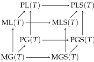
ML(T)_i:={t_i∈T_i:¬∃µ_i∈∆(T_i)µ_i>_Tt_i}, MG(T)_i:={ti∈Ti:¬∃^µi∈∆(Si)µ_i>_Tti}, PL(T)_i:={t_i∈T_i:¬∃t^′_i∈T_it^′_i>_Tt_i}, and PG(T)_i:={ti∈Ti:¬∃si∈Sisi>_Tti}.

MLS, MGS, PLS, PGS are defined analogously with≫Tinstead of>_T. For allTwe have the following obvious inclusions:

• Every M-operator eliminates more strategies than the corresponding P-operator.

4.5 Iterated Elimination of Dominated Strategies

• Every operator considering (weak) dominance eliminates more strategies than the corresponding operator considering strict dominance.

• With dominance in global games more strategies are eliminated than with dominance in local games.

MG(T) MGS(T) ML(T) MLS(T)

PG(T) PGS(T) PL(T) PLS(T)

Figure 4.1.Inclusions between the eight strategy elimination operators Each of these operators is deflationary, i.e. F(T)⊆Tfor everyT and every operatorF. We iterate an operator beginning withT= S, i.e. F⁰:=SandF^α+1:=F(F^α). Obviously,F⁰⊇F¹⊇ · · · ⊇F^α⊇F^α+1. SinceSis finite, we will reach a fixed pointF^αsuch thatF^α=F^α+1=:F^∞. We expect that for the eight fixed points MG^∞, ML^∞, etc. the same inclusions hold as for the operators MG(T), ML(T), etc. But this is not the case: For the following gameΓ= ({0, 1},(S0,S1),(p0,p1))we have ML^∞⊈PL^∞.

X Y Z

A (2, 1) (0, 1) (1, 0) B (0, 1) (2, 1) (1, 0) C (1, 1) (1, 0) (0, 0) D (1, 0) (0, 1) (0, 0) We have:

•Zis dominated byXandY.

•Dis dominated byA.

•Cis dominated by¹₂A+¹₂B.

Thus:

(10)

ML(S) =ML¹= ({A,B},{X,Y})⊂PL(S) =PL¹

= ({A,B,C},{X,Y}). ML(ML¹) =ML¹since in the following game there are no dominated strategies:

X Y

A (2, 1) (0, 1) B (0, 1) (2, 1)

PL(PL¹) = ({A,B,C},{X}) =PL²⫋PL¹sinceYis dominated by X(here we need the presence ofC). SinceBandCare now dominated byA, we have PL³= ({A},{X}) =PL^∞. Thus, PL^∞⫋ML^∞although ML is the stronger operator.

We are interested in the inclusions of the fixed points of the different operators. But we only know the inclusions for the operators. So the question arises under which assumptions can we prove, for two deflationary operatorsFandGonS, the following claim:

IfF(T)⊆G(T)for allT, thenF^∞⊆G^∞?

The obvious proof strategy is induction overα: We haveF⁰=G⁰=S, and ifF^α⊆G^α, then

F^α+1=F(F^α)⊆G(F^α) F(G^α)⊆G(G^α) =G^α+1

If we can show one of the inclusionsF(F^α)⊆ F(G^α)orG(F^α) ⊆ G(G^α), then we have proven the claim. These inclusions hold if the operators are monotone: H : S → Sis monotone if T ⊆ T^′implies H(T)⊆H(T^′). Thus, we have shown:

Lemma 4.18. Let F,G : P(S) → P(S)be two deflationary operators such thatF(T)⊆G(T)for allT⊆S. If eitherForGis monotone, then F^∞⊆G^∞.

Corollary 4.19. PL and ML are not monotone on every game.

4.5 Iterated Elimination of Dominated Strategies Which operators are monotone? Obviously, MGS and PGS are monotone: Ifµ_i≫Ts_iandT^′⊆T, then alsoµ_i≫T^′s_i. LetT^′⊆Tand si∈PGS(T^′)_i. Thus, there is noµ_i∈Sisuch thatµ_i≫T^′ si, and there is also noµ_i ∈S_isuch thatµ_i≫T s_iand we haves_i∈PGS(T)_i. The reasoning for MGS is analogous if we replaceSiby∆(Si).

MLS and PLS are not monotone. Consider the following simple game:

X A (1, 0) B (0, 0)

MLS({A,B},{X}) =PLS({A,B},{X}) = ({A},{X})and MLS({B},{X}) =PLS({B},{X}) = ({B},{X}), but({B},{X})̸⊆({A},{X}).

Thus, none of the local operators (those which only consider dominant strategies in the current subgame) is monotone. We will see that also MG and PG are not monotone in general. The monotonicity of the global operators MGS and PGS will allow us to prove the expected inclusions ML^∞⊆MLS^∞⊆PLS^∞and PL^∞⊆PLS^∞between the local operators. To this end, we will show that the fixed points of the local and corresponding global operators coincide (although the operators are different).

Lemma 4.20.MGS^∞=MLS^∞and PGS^∞=PLS^∞.

Proof. We will only prove PGS^∞=PLS^∞. Since PGS(T)⊆PLS(T)for allT and PGS is monotone, we have PGS^∞ ⊆ PLS^∞. Now we will prove by induction that PLS^α⊆PGS^αfor allα. Only the induction step α7→α+1 has to be considered: Lets_i∈PLS^α+1_i . Therefore,s_i∈PLS^α_i and there is nos^′_i∈PLS_i^αsuch thats^′_i≫_PLS^αsi. Assumesi∈/PGS^α+1_i , i.e.

A={s^′_i∈S_i:s^′_i≫PGS^αs_i} ̸=∅

(note: By induction hypothesis PGS^α =PLS^α). Pick ans^∗_i ∈ Awhich is maximal with respect to≫PLS^α. Claim:s^∗_i ∈PLS^α. Otherwise, there

(11)

exists aβ ≤αand ans_i′ ∈Siwiths^′_i ≫_PLS^β si^∗. Since PLS^β ⊇ PLS^α, it follows thats^′_i ≫PLS^α s^∗_i ≫PLS^α s_i. Therefore,s_i^′∈ Aands^∗_i is not maximal with respect to≫_PLS^αinA. Contradiction.

But ifs^∗_i ∈PLS^α ands^∗_i ≫PLS^α s_i, thens_i ∈/PLS^α+1which again constitutes a contradiction.

The reasoning for MGS^∞and MLS^∞is analogous. q.e.d.

Corollary 4.21. MLS^∞⊆PLS^∞.

Lemma 4.22.MG^∞=ML^∞and PG^∞=PL^∞.

Proof. We will only prove PG^∞=PL^∞by proving PG^α=PL^αfor allα by induction. Let PG^α=PL^αands_i∈PG^α+1_i . Thens_i∈PG^α_i =PL^α_i and hence there is nos^′_i∈Sisuch thats^′_i>_PG^αsi. Thus, there is nos^′_i∈PL^α_i such thats^′_i>_PL^αs_iands_i∈PL^α+1. So, PG^α+1⊆PL^α+1.

Now, letsi ∈ PL^α+1_i . Again we havesi ∈ PL^α_i = PG^α_i. Assume si/∈PG^α+1_i . Then

A={s^′_i∈Si:s^′_i>_PL^αsi} ̸=∅.

For everyβ≤αletA^β=A∩PL^β_i. Pick the maximalβsuch thatA^β̸=∅ and as^∗_i ∈A^βwhich is maximal with respect to>_PLβ.

Claim: β=α. Otherwise,s_i^∗̸∈PL^β+1_i . Then there exists ans^′_i∈PL^β_i withs^′_i>_PLβs^∗_i. Since PL^β⊇PL^αands_i^∗>_PL^αsi, we haves^′_i>_PL^αsi, i.e.

s^′_i∈A^βwhich contradicts the choice ofs^∗_i. Therefore,s^∗_i ∈PL^α_i. Since s^∗_i >_PL^α s_i, we haves_i /∈PL^α+1_i . Contradiction, hence the assumption is wrong, and we havesi∈PG^α+1. Altogether PG^α=PL^α. Again, the reasoning for MG^∞=ML^∞is analogous. q.e.d.

Corollary 4.23. PL^∞⊆PLS^∞and ML^∞⊆MLS^∞.

Proof. We have PL^∞ = PG^∞ ⊆ PGS^∞ = PLS^∞ where the inclusion PG^∞ ⊆PGS^∞ holds because PG(T) ⊆PGS(T)for any Tand PGS is monotone. Analogously, we have ML^∞ = MG^∞ ⊆ MGS^∞ = MLS^∞. q.e.d.

This implies that MG and PG cannot be monotone. Otherwise, we would have ML^∞=PL^∞. But we know that this is wrong.

4.6 Beliefs and Rationalisability

LetΓ= (N,(S_i)_i∈N,(p_i)_i∈N)be a game. Abeliefof Playeriis a probability distribution overS−i.

Remark4.24.A belief is not necessarily a product of independent probability distributions over the individualSj(j̸=i). A player may believe that the other players play correlated.

A strategysi∈Siis called abest response to a beliefγ∈∆(S−i)if pb_i(s_i,γ) ≥ pb_i(s^′_i,γ)for all s^′_i ∈ S_i. Conversely, s_i ∈ S_iisnever a best responseifsiis not a best response for anyγ∈∆(S−i).

Lemma 4.25.For every gameΓ= (N,(Si)_i∈N,(pi)_i∈N)and everysi∈Si, siis never a best response if and only if there exists a mixed strategy µ_i∈∆(S_i)such thatµ_i≫Ss_i.

Proof. Ifµ_i≫S si, then pbi(µ_i,s−i)> pbi(si,s−i)for alls−i∈S−i. Thus, pbi(µi,γ)>p_bi(si,γ)for allγ∈∆(S₋i). Then, for every beliefγ∈∆(S₋i), there exists ans_i^′∈supp(µ_i)such thatpb_i(s^′_i,γ)>p_b_i(s_i,γ). Therefore,s_i is never a best response.

Conversely, lets^∗_i ∈Sibe never a best response inΓ. We define a two-person zero-sum gameΓ^′= ({0, 1},(T0,T₁),(p,−p))whereT0= Si− {s^∗_i},T1=S−iandp(si,s−i) = pi(si,s−i)−pi(s^∗_i,s−i). Sinces^∗_i is never a best response, for every mixed strategyµ1∈∆(T1) = ∆(S₋i) there is a strategys₀∈T₀=S_i− {s^∗_i}such thatpb_i(s₀,µ₁)> p_b_i(s^∗_i,µ₁) (inΓ), i.e.p(s0,µ₁)>0 (inΓ^′). So, inΓ^′

µ1min∈∆(T1)max

s0∈T0p(s0,µ₁)>0, and therefore

µ1min∈∆(T1) max

µ0∈∆(T0)p(µ0,µ1)>0.

By Nash’s Theorem, there is a Nash equilibrium(µ₀^∗,µ^∗₁)inΓ^′. By von Neumann and Morgenstern we have

µ1min∈∆(T1) max

s0∈∆(T0)p(µ₀,µ₁) =p(µ^∗₀,µ^∗₁)

(12)

= max

s0∈∆(T0) min

µ1∈∆(T1)p(µ0,µ₁)>0.

Thus, 0 < p(µ^∗₀,µ^∗₁) ≤ p(µ^∗₀,µ₁) for all µ₁ ∈ ∆(T₁) = ∆(S_−i). So, we have inΓ pbi(µ^∗₀,s_−i) > pi(s^∗_i,s_−i)for alls−i ∈ S−i which means

µ^∗₀≫Ss^∗_i. q.e.d.

Definition 4.26. Let Γ = (N,(Si)_i∈N,(pi)_i∈N)be a game. A strategy si∈SiisrationalisableinΓif for any Playerjthere exists a setTj⊆Sj

such that

•s_i∈T_i, and

• everysj∈ Tj(for allj) is a best response to a beliefγ_j ∈∆(S−j) where supp(γj)⊆T₋j.

Theorem 4.27.For every finite gameΓwe have: s_iis rationalisable if and only ifsi ∈MLS^∞_i . This means, the rationalisable strategies are exactly those surviving iterated elimination of strategies that are strictly dominated by mixed strategies.

Proof. Letsi∈Sibe rationalisable byT= (T1, . . . ,Tn). We showT⊆ MLS^∞. We will use the monotonicity of MGS and the fact that MLS^∞= MGS^∞. This implies MGS^∞ =gfp(MGS)and hence, MGS^∞contains all other fixed points. It remains to show that MGS(T) = T. Every s_j ∈ T_jis a best response (among the strategies inS_j) to a beliefγ with supp(γ) ⊆ T−j. This means that there exists no mixed strategy µj∈∆(Sj)such thatµj≫Tsj. Therefore,sjis not eliminated by MGS:

MGS(T) =T.

Conversely, we have to show that every strategy s_i ∈ MLS^∞_i is rationalisable by MLS^∞. Since MLS^∞=MGS^∞, we have MGS(MLS^∞) = MLS^∞. Thus, for every si ∈MLS^∞_i there is no mixed strategyµi ∈

∆(S_i) such thatµ_i ≫MLS^∞ s_i. So, s_i is a best response to a belief in

MLS^∞_i. q.e.d.

Intuitively, the concept of rationalisability is based on the idea that every player keeps those strategies that are a best response to a possible combined rational action of his opponents. As the following example shows, it is essential to also consider correlated actions of the players.

4.6 Beliefs and Rationalisability Example4.28.Consider the following cooperative game in which every player receives the same payoff:

L R L R L R L R

T 8 0 4 0 0 0 3 3

B 0 0 0 4 0 8 3 3

1 2 3 4

Matrix 2 is not strictly dominated. Otherwise there werep,q∈[0, 1] withp+q≤1 and

8·p+3·(1−p−q)>4 and 8·q+3·(1−p−q)>4.

This implies 2·(p+q) +6>8, i.e. 2·(p+q)>2, which is impossible.

So, matrix 2 must be a best response to a beliefγ∈∆({T,B} × {L,R}). Indeed, the best responses to γ = ¹₂·((T,L) + (B,R))are matrices 1, 2 or 3.

On the other hand, matrix 2 is not a best response to a belief of independent actionsγ∈∆({T,B})×∆({L,R}). Otherwise, if matrix 2 were a best response toγ= (p·T+ (1−p)·B,q·L+ (1−q)·R), we would have that

4pq+4·(1−p)·(1−q)≥max{8pq, 8·(1−p)·(1−q), 3}. We can simplify the left side: 4pq+4·(1−p)·(1−q) =8pq−4p−4q+ 4. Obviously, this term has to be greater than each of the terms from which we chose the maximum:

8pq−4p−4q+4≥8pq⇒p+q≥1 and

8pq−4p−4q+4≥8·(1−p)·(1−q)⇒p+q≤1.

So we havep+q=1, orq=1−p. But this allows us to substituteqby 1−p, and we get

8pq−4p−4q+4=8p·(1−p).

(13)

However, this term must still be greater or equal than 3, so we get 8p·(1−p)≥3

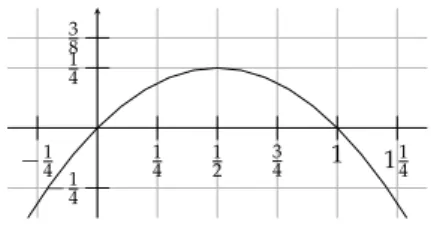
⇔p·(1−p)≥³₈,

which is impossible since max(p·(1−p)) =¹₄(see Figure 4.2).

14 38

−¹₄

−¹₄ ¹₄ ¹₂ ³₄ ¹ 1¹₄

Figure 4.2.Graph of the functionp7→^p·(1−^p)

4.7 Games in Extensive Form

Agame in extensive form(with perfect information) is described by a game tree. For two-person games this is a special case of the games on graphs which we considered in the earlier chapters. The generalisation ton-person games is obvious: G= (V,V1, . . . ,Vn,E,p1, . . . ,pn)where (V,E)is a directed tree (with root nodew),V=V1⊎ · · · ⊎Vn, and the payoff functionp_i: Plays(G)→^Rfor Playeri, where Plays(G)is the set of paths through(V,E)beginning in the root node, which are either infinite or end in a terminal node.

A strategy for PlayeriinGis a function f:{v∈V_i:vE̸=∅} →V such that f(v) ∈ vE. Siis the set of all strategies for Playeri. If all players 1, . . . ,neach fix a strategyfi∈Si, then this defines a unique play

f₁ˆ· · ·ˆfn∈Plays(G).

We say thatGhasfinite horizonif the depth of the game tree (the length of the plays) is finite.

For every game G in extensive form, we can construct a game S(G) = (N,(Si)_i_∈_N,(pi)_i_∈_N)with N= {1, . . . ,n}andpi(f1, . . . ,fn) = p_i(f1ˆ· · ·ˆfn). Hence, we can apply all solution concepts for strategic

4.7 Games in Extensive Form games (Nash equilibria, iterated elimination of dominated strategies, etc.) to games in extensive form. First, we will discuss Nash equilibria in extensive games.

Example4.29. Consider the gameG(of finite horizon) depicted in Fig- ure 4.3 presented as (a) an extensive-form game and as (b) a strategic- form game. The game has two Nash equilibria:

• The natural solution(b,d)where both players win.

• The second solution(a,c)which seems to be irrational since both players pick an action with which they lose.

What seems irrational about the second solution is the following observation. If Player 0 picksa, it does not matter which strategy her opponent chooses since the positionvis never reached. Certainly, if Player 0 switches fromatob, and Player 1 still responds withc, the payoff of Player 0 does not increase. But this threat is not credible since ifvis reached after actiona, then actiondis better for Player 1 thanc.

Hence, Player 0 has an incentive to switch fromatob.

w

(0, 1) a

v

(0, 0) c

(1, 1) d b

(a) extensive form

c d

a (0, 1) (0, 1) b (0, 0) (1, 1)

(b) strategic form Figure 4.3.A game of finite horizon

This example shows that the solution concept of Nash equilibria is not sufficient for games in extensive form since they do not take the sequential structure into account. Before we introduce a stronger notion of equilibrium, we will need some more notation: LetGbe a game in extensive form andva position ofG. G↾vdenotes thesubgameofG beginning inv(defined by the subtree ofGrooted atv). Payoffs: Let hvbe the unique path fromwtovinG. Thenp^G↾_i ^v(π) =p^G_i(hv·π). For every strategyfof PlayeriinGletf↾vbe the restriction offtoG↾v.

(14)

Definition 4.30. Asubgame perfect equilibriumofGis a strategy profile (f₁, . . . ,fn)such that, for every positionv, (f₁↾v, . . . ,fn↾v)is a Nash equilibrium ofG↾v. In particular,(f1, . . . ,fn)itself is a Nash equilibrium.

In the example above, only the natural solution(b,d)is a subgame perfect equilibrium. The second Nash equilibrium(a,c)is not a subgame perfect equilibrium since(a↾v,c↾v)is not a Nash equilibrium inG↾v.

LetGbe a game in extensive form, f = (f1, . . . ,fn)be a strategy profile, andva position inG. We denote by ef(v)the play inG↾vthat is uniquely determined by f1. . . ,fn.

Lemma 4.31. Let G be a game in extensive form with finite horizon.

A strategy profile f= (f1, . . . ,fn)is a subgame perfect equilibrium of G if and only if for every Playeri, everyv ∈ Vi, and everyw ∈ vE:

pi(ef(v))≥pi(ef(w)).

Proof. Let f be a subgame perfect equilibrium. Ifpi(^ef(w))> pi(^ef(v)) for somev∈Vi,w∈vE, then it would be better for PlayeriinG↾vto change her strategy invfromf_ito f_i^′with

f_i^′(u) =





fi(u) ifu̸=v w ifu=w. This is a contradiction.

Conversely, iffis not a subgame perfect equilibrium, then there is a Playeri, a positionv0∈Viand a strategy f_i^′̸= fisuch that it is better for PlayeriinG↾v0to switch fromfito f_i^′against f₋i. Letg:= (f_i^′,f₋i). We haveq:=p_i(_eg(v0))>p_i(ef(v0)). We consider the patheg(v0) =v0. . .vt

and pick a maximalm<twithpi(_eg(v0))>pi(^ef(vm)). Choosev=vm

andw=vm+1∈vE. Claim:pi(ef(v))<pi(ef(w))(see Figure 4.4):

pi(^ef(v)) =pi(^ef(vm))<pi(eg(vm)) =q

pi(ef(w)) =pi(ef(vm+1))≥pi(g_e(vm+1)) =q q.e.d.

Iffis not a subgame perfect equilibrium, then we find a subgame G↾vsuch that there is a profitable deviation from fiinG↾v, which only differs from f_iin the first move.

4.7 Games in Extensive Form v0

<q

vm=v

<q

v_m+1=w

≥q

q ge(v0) ef(v₀)

ef(vm)

ef(vw)

Figure 4.4.pi(fe(v))<pi(ef(w))

In extensive games with finite horizon we can directly define the payoff at the terminal nodes (the leaves of the game tree). We obtain a payoff functionpi:T→^Rfori=1, . . . ,nwhereT={v∈V:vE=∅}.

Backwards induction: For finite games in extensive form we define a strategy profilef= (f1, . . . ,fn)and valuesui(v)for all positionsvand every Playeriby backwards induction:

• For terminal nodest∈Twe do not need to define f, andu_i(t):= pi(t).

• Letv∈V\Tsuch that allu_i(w)for alliand allw∈vEare already defined. Foriwith v ∈ Vi define fi(v) = w for some w with ui(w) =max{ui(w^′):w^′∈vE}anduj(v):=uj(fi(v))for allj.

We havep_i(ef(v)) =u_i(v)for everyiand everyv.

Theorem 4.32. The strategy profile defined by backwards induction is a subgame perfect equilibrium.

Proof. Let f_i^′ ̸= fi. Then there is a nodev0∈Viwith minimal height in the game tree such that f_i^′(v)̸= fi(v). Especially, for everyw∈vE, (^f_i^′,f₋i)(w) =fe(w). Forw=f_i^′(v)we have

pi((^f_i^′,f−i)(v)) = pi((^f_i^′,f−i)(w))

= pi(ef(w))

= ui(w)≤ max

w^′∈vE{ui(w^′)}

(15)

= ui(v)

= pi(^ef(v)).

Therefore, f↾vis a Nash equilibrium inG↾v. q.e.d.

Corollary 4.33. Every finite game in extensive form has a subgame perfect equilibrium (and thus a Nash equilibrium) in pure strategies.

4.8 Subgame-perfect equilibria in infinite games

We now consider cases of infinite games in extensive form, for which we can establish the existence of subgame-perfect equilibria. General- izing the model of infinite two-person zero-sum games on graphs, we consider multi-player, turn-based games on graphs with arbitrary (not necesssarily antagonistic) qualitative objectives.

Definition 4.34. Aninfinite (turn-based, qualitative) multiplayer gameis a tupleG = (N,V,(Vi)_i∈N,E,Ω,(Wini)_i∈N)whereNis a finite set of players,(V,E)is a (finite or infinite) directed graph(V_i)_i∈Nis a partition ofVinto the position sets for each player,Ω:V →Cis a colouring of the positions by some finite setCof colours, and Wini⊆C^ωis the winning condition for Playeri.

For the sake of simplicity, we assume thatuE:={v∈V:(u,v)∈ E} ̸=∅for allu∈V, i.e. each vertex ofGhas at least one outgoing edge. We callGazero-sum gameif the sets Win_idefine a partition ofC^ω. Aplay of G is an infinite path through the graph(V,E), and a historyis a finite initial segment of a play. We say that a playπ is won by PlayeriifΩ(π) ∈ Win_i. A (pure) strategy of Player i inG is a function f : V^∗Vi → V assigning to each sequencexv ending in a positionvof Playeria next position f(xv)∈vE. We say that a play π = π(0)π(1). . . ofG is consistentwith a strategy f of Player iif π(k+1) = f(π(0). . .π(k))for allk< ωwith π(k) ∈Vi. Astrategy profileofGis a tuple(fi)_i_∈_Nwherefiis a strategy of Playeri.

It is sometimes convenient to designate an initial vertexv0 ∈V of the game. We call the tuple(G,v0)aninitialized infinite multiplayer game. Aplay (history) of(G,v0)is a play (history) ofGstarting withv0.

4.8 Subgame-perfect equilibria in infinite games A strategy (strategy profile) of(G,v0)is just a strategy (strategy profile) ofG. A strategyfof some playeriin(G,v₀)iswinningif every play of (G,v0)consistent withσis won by playeri. A strategy profile(fi)_i∈N of(G,v0)determines a unique play of(G,v0)consistent with each f_i, called theoutcome of(fi)_i∈Nand denoted by⟨(fi)_i∈N⟩or, in the case that the initial vertex is not understood from the context,⟨(fi)_i_∈_N⟩v0. In the following we will often use the termgameto denote an(initialized) infinite multiplayer gameaccording to Definition 4.34.

For turn-based (non-stochastic) games with qualitative winning conditions, mixed strategies play no relevant role. Nash equilibria in pure strategies take the following form:

A strategy profile(fi)_i_∈_Nof a game(G,v0)is aNash equilibriumif for every player i and all her possible strategies f_i^′in(G,v0)the play

⟨f_i^′,(fj)_j∈N\{i}⟩is won by playerionly if the play⟨(fj)_j∈N⟩is also won by her.

Despite the importance and popularity of Nash equilibria, there are several problems with this solution concept, in particular for games that extend over time. This is due to the fact that Nash equilibria do not take into account the sequential nature of games and all the consequences of this. After any initial segment of a play, the players face a new situation and may change their strategies. Choices made because of a threat by the other players may no longer be rational, because the opponents have lost their power of retaliation in the remaining play.

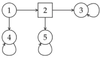
Example4.35. Consider a two-player Büchi game with its arena depicted in Figure 4.5; round vertices are controlled by player 1; boxed vertices are controlled by player 2; both players win if and only if vertex 3 is visited (infinitely often); the initial vertex is 1. Intuitively, the only rational outcome of this game should be the play 123^ω. However, the game has two Nash equilibria:

(1) Player 1 moves from vertex 1 to vertex 2, and player 2 moves from vertex 2 to vertex 3. Hence, both players win.

(2) Player 1 moves from vertex 1 to vertex 4, and player 2 moves from vertex 2 to vertex 5. Both players lose.

The second equilibrium certainly does not describe a rational be- haviour. Indeed both players move according to a strategy that is always

4 Basic Concepts of Mathematical

Logic and Games WS 2015/2016

Prof. Dr. Erich Grädel

c b n d

Contents

4 Basic Concepts of Mathematical

Game Theory

4.1 Games in Strategic Form

4.2 Nash equilibria

∑

∏

∑

∑

∑

∑

4.3 Two-person zero-sum games

4.4 Regret minimization

4.5 Iterated Elimination of Dominated Strategies

4.6 Beliefs and Rationalisability

4.7 Games in Extensive Form

4.8 Subgame-perfect equilibria in infinite games