The Simple Geometry of Perfect Information Games

IHS Economics Series Working Paper 115

June 2002

The Simple Geometry of Perfect Information Games

Stefano Demichelis

Klaus Ritzberger

Jeroen M. Swinkels

Impressum Author(s):

Stefano Demichelis, Klaus Ritzberger, Jeroen M. Swinkels Title:

The Simple Geometry of Perfect Information Games ISSN: Unspecified

2002 Institut für Höhere Studien - Institute for Advanced Studies (IHS) Josefstädter Straße 39, A-1080 Wien

E-Mail: o ce@ihs.ac.atffi Web: ww w .ihs.ac. a t

All IHS Working Papers are available online: http://irihs. ihs. ac.at/view/ihs_series/

This paper is available for download without charge at:

The Simple Geometry of Perfect Information Games

Stefano Demichelis, Klaus Ritzberger, Jeroen M. Swinkels

115

Reihe Ökonomie

Economics Series

115 Reihe Ökonomie Economics Series

The Simple Geometry of Perfect Information Games

Stefano Demichelis, Klaus Ritzberger, Jeroen M. Swinkels June 2002

Institut für Höhere Studien (IHS), Wien

Contact:

Stefano Demichelis CORE

34, Voie du Roman Pays

B-1348 Louvain-la-Neuve; Belgium email: stefano@core.ucl.ac.be

Klaus Ritzberger

Institute for Advanced Studies Department of Economics and Finance Stumpergasse 56

A-1060 Vienna, Austria (: +43/1/599 91-153 fax: +43/1/599 91-163 email: ritzbe@ihs.ac.at

Jeroen M. Swinkels

John M. Olin School of Business Washington University at St. Louis St. Louis, MO 63005, USA

email: swinkels@mail.olin.wustl.edu

Founded in 1963 by two prominent Austrians living in exile – the sociologist Paul F. Lazarsfeld and the economist Oskar Morgenstern – with the financial support from the Ford Foundation, the Austrian Federal Ministry of Education and the City of Vienna, the Institute for Advanced Studies (IHS) is the first institution for postgraduate education and research in economics and the social sciences in Austria.

The Economics Series presents research done at the Department of Economics and Finance and aims to share “work in progress” in a timely way before formal publication. As usual, authors bear full responsibility for the content of their contributions.

Das Institut für Höhere Studien (IHS) wurde im Jahr 1963 von zwei prominenten Exilösterreichern – dem Soziologen Paul F. Lazarsfeld und dem Ökonomen Oskar Morgenstern – mit Hilfe der Ford- Stiftung, des Österreichischen Bundesministeriums für Unterricht und der Stadt Wien gegründet und ist somit die erste nachuniversitäre Lehr- und Forschungsstätte für die Sozial- und Wirtschafts - wissenschaften in Österreich. Die Reihe Ökonomie bietet Einblick in die Forschungsarbeit der Abteilung für Ökonomie und Finanzwirtschaft und verfolgt das Ziel, abteilungsinterne Diskussionsbeiträge einer breiteren fachinternen Öffentlichkeit zugänglich zu machen. Die inhaltliche

Abstract

Perfect information games have a particularly simple structure of equilibria in the associated normal form. For generic such games each of the finitely many connected components of Nash equilibria is contractible. For every perfect information game there is a unique connected and contractible component of subgame perfect equilibria. Finally, the graph of the subgame perfect equilibrium correspondence, after a very mild deformation, looks like the space of perfect information extensive form games.

Keywords

Perfect information, subgame perfection, equilibrium correspondence

JEL Classifications

C72

Contents

1. Introduction 1

2. Definitions and Notation 4

3 Generic Perfect Information Games 7

4 Subgame Perfect Equilibria 15

5 Conclusions 24

6 Appendix 24

References 29

1 Introduction

Perfect information games have played an important role in the development of game theory. One of the earliest existence proofs for Nash equilibrium was given for this class of games (Kuhn (1953)). Perfect information games have guided equilibrium selection in applied models with multiple equilibria well before the re…nement debate came into swing (Selten (1965)). They have provided the playground for the idea of backwards induction in its various forms. Last, but not least, they have been applied to a large number of im- portant economic problems: bilateral bargaining, Stackelberg duopoly, wage and employment determination (Leontief (1946)), monetary policy (Barro and Gordon (1983)), and numerous other models in industrial organization.

The reason for this prominence is because of the simplicity of perfect information games. Of course, this is also the reason that perfect informa- tion is considered such a restrictive assumption in modern game theory. Such games have the highest possible degree of decomposability. Every move is the root of a subgame that can in principle be analyzed separately. This invites the application of a backwards induction or “dynamic programming” proce- dure. (Incidentally, perfect information games have also been used to show that such procedures do not necessarily yield intuitive results; see Rosenthal (1981) on the chain-store paradox.)

Recently, a further application for perfect information games has surfaced at the intersection of equilibrium selection theory and evolutionary game the- ory. As an alternative to rationality-based re…nements of Nash equilibrium, evolutionary game theorists argue that equilibria should be selected that have certain dynamic (or stochastic) stability properties in evolutionary selection dynamics. (For an overview on evolutionary game theory see Weibull (1995) or Samuelson (1997).)

Quite a number of results are already available in this …eld. Though most refer to normal form games, many use the normal forms of perfect information games as their benchmarks and for illustrations. The spirit of the exercise is that an evolutionary selection of the subgame perfect equilibrium outcome in perfect information games provides a justi…cation for backwards induction independent of issues of rationality. Moreover, perfect information games are su¢ciently simple to allow for …rst advances in the theory of evolution on extensive form games. (See Nöldeke and Samuelson (1993) for an interesting analysis in more general extensive form games.)

Cressman and Schlag (1998) and Hart (1999) identify conditions for when

evolution will select the backwards induction solution in (the normal forms of) perfect information games. In other approaches the results on backwards induction are more implicit. For example, Marx (1999) shows conditions under which iterated weak dominance is implied by an adaptive dynamic.

Of course, iterated weak dominance selects the backward induction outcome in games of perfect information.

Frequently, results about backward induction are implied by results on strategic stability (see Swinkels (1992) and (1993), Ritzberger and Weibull (1995), and Demichelis and Ritzberger (2000)). But such indirect conclusions depend heavily on the structure of the equilibrium set. The well-known uniqueness of subgame perfect equilibrium in generic perfect information games is helpful here, but often not su¢cient, because in the normal form the whole component of Nash equilibria that induces the backwards induction outcome has to be considered.

In this paper, we aim at a complete description of the structure of the equilibrium set for perfect information games. Three results are presented.

First, for generic perfect information games all components of Nash equilib- ria are contractible. For such games with only two players they are convex.

Moreover, each component will contain a pure equilibrium, whatever the number of players. Second, every perfect information games, even if degen- erate, has only one component of equilibria that contains subgame perfect ones; and this component is also contractible. This, together with uniqueness for generic games, already suggests that the subgame perfect equilibrium cor- respondence on the space of perfect information games is rather simply. Our third result shows that an arbitrary small deformation of the graph makes it

“look like” (viz. project homeomorphically onto) the space of games.

There are important applications of these insights. In a recent paper

Demichelis and Ritzberger ((2000), Theorem 1) show that for a component

of Nash equilibria to be asymptotically stable in an evolutionary (determin-

istic continuous-time) selection dynamics (acting on the normal form) it is

necessary that its index (Ritzberger (1994)) coincides with its Euler char-

acteristic. (This is a substantial weakening of an analogous condition used

by Swinkels (1993).) They apply this to two-player outside-option games

(as introduced by van Damme (1989)) to show that, if it selects an outcome

at all, evolution will select the forward induction outcome. (This result on

dynamics is analogous to the result obtained by Hauk and Hurkens (forth-

coming) in a static context.) But there are outside-option games where for

no component the index does agree with the Euler characteristic.

The present result implies that for generic perfect information games the situation is better: for the backwards induction component the index will always agree with the Euler characteristic. This is because for generic perfect information games we show that all components are contractible and thus have Euler characteristic +1. The index assignment is very easy for such games: since every component with nonzero index contains a Mertens-stable set (Demichelis and Ritzberger (2000), Theorem 2), the backwards induction component has index +1 and all other components of equilibria have index 0.

To see this, note that if any other than the backwards induction component had nonzero index, it would contain a Mertens-stable set (for a de…nition see Mertens (1989) and (1991)). Since any Mertens-stable set contains a proper equilibrium (Myerson (1978)) and any proper equilibrium induces a sequential (hence, subgame perfect) equilibrium in any compatible normal form (van Damme (1984); Kohlberg and Mertens (1986)), such an other component would contain a subgame perfect equilibrium, in contradiction to uniqueness of the latter. That the backwards induction component has index +1 then follows from the property that the sum of the index across all components is +1.

That components of equilibria are contractible does not extend to degen- erate perfect information games. A counterexample is given below. But when attention is restricted to subgame perfect equilibria, the result is resurrected.

Even for degenerate perfect information games the unique component that consists of subgame perfect equilibria is contractible.

Degenerate perfect information games are of considerable interest in con- sidering the properties of the subgame perfect equilibrium correspondence.

At generic points, the subgame perfect equilibrium correspondence is a func- tion. Hence, the behavior of the correspondence at degenerate games deter- mines its properties. To clarify this issue, we prove a result analogous to the structure-theorem by Kohlberg and Mertens ((1986), Theorem 1): the graph of the subgame perfect equilibrium correspondence can be continu- ously deformed into the space of perfect information games. In particular, the subgame perfect equilibrium correspondence is upper hemi-continuous.

The rest of the paper is organized as follows. Section 2 gives basic de-

…nitions. In Section 3 it is shown that all components are contractible in

the generic case. Section 4 focuses on subgame perfect equilibria and con-

tains the other two results. Section 5 concludes. An appendix contains a

discussion of the relation between mixed and behavior strategies.

2 De…nitions and Notation

The following basic de…nitions for extensive form games are used through- out. A tree T is a …nite connected directed graph without loops and with a distinguished node, called the root, that comes before all other nodes. Nodes that have no successors are called terminal, and all other nodes are called moves. The set of all nodes is denoted by N , the set of moves by X, and the root by x

2 X.

On a tree T de…ne the immediate predecessor function P : N n f x

g ! X by the condition that P (x) 2 X n f x g comes before x 2 N and all nodes that come before x come before P (x) or coincide with it, for all x 2 N . That is, the immediate predecessor P (x) of x is the “latest” node that comes before x. By convention, extend P to N , setting P (x

) = x

. By …niteness, for every x 2 N there is some t = 1; 2; ::: such that P

(x) = P (P

(x)) = x

, where P

is the identity. Hence, x 2 N comes before y 2 N if and only if there is t = 1; 2; ::: such that x = P

(y).

De…nition 1 An n-player extensive form with perfect information is a triple F = (T; X ; p), where

² T is a tree,

² X = (X

; X

; :::; X

) is a partition of X into decision points,

² p : P

(X

) ! R

is a function such that X

y2P^¡1(x)

p (y) = 1 for all x 2 X

(1) which assigns probabilities to (immediate successors of ) chance moves x 2 X

, where P

(x) = f y 2 N j P (y) = x g for all x 2 X and P

(X

) ´ [

P

(x).

Moves in X

´ [

X

are decision points of personal players, moves

in X

are chance moves. A choice for player i is a node y 2 P

(x) for

some move x 2 X

. A play is a maximal chain (completely ordered subset)

of nodes that starts with the root and ends with a terminal node. Let W

denote the set of plays for the tree T . By …niteness, terminal nodes and plays

are one-to-one.

An n-player perfect information extensive form game is a pair G = (F; v), where F is an n-player extensive form with perfect information and v = (v

; :::; v

) : W ! R

is the payo¤ function. A subgame G

of a perfect information game G is the extensive form game obtained by restricting G to the tree rising at x 2 X.

A pure strategy for player i = 1; :::; n in an n-player perfect information extensive form game G is a function s

: X

! N such that

P (s

(x)) = x for all x 2 X

(2) That is, a pure strategy assigns a “next” node for each move belonging to i. The set of all pure strategies of player i is denoted by S

: The product S = S

£ ::: £ S

is the set of all pure strategy combinations.

A mixed strategy for player i is a probability distribution ¾

on S

, and

¢

denotes the simplex of all mixed strategies for player i. The product

£ = ¢

£ ::: £ ¢

is the set of all mixed strategy combinations.

A behavior strategy for player i is a function b

: P

(X

) ! R

,where P

(X

) ´ [

P

(x), such that

X

y2P^¡1(x)

b

(y) = 1 for all x 2 X

(3) and B

denotes the set of all behavior strategies for player i - a product of j X

j simplices. The subvector (b

(y))

for some move x 2 X

will be referred to as behavior of player i at x. The product B = B

£ ::: £ B

is the set of all behavior strategy combinations.

Every pure or behavior strategy combination induces (together with p) a unique transition probability to a node from its immediate predecessor.

Multiplying transition probabilities over all predecessors of a node induces a nonnegative real-valued function ¼ on nodes that assigns the probability

¼ (x) of node x 2 N being reached (from the root). From this, a unique probability distribution ¼ : W ! R

on plays is obtained, by selecting the corresponding terminal nodes. This distribution on plays is the outcome associated with the pure or behavior strategy combination.

Due to the structure of a tree, the basic relation between the outcome

¼ = (¼ (w))

and the probability ¼ (x) of a node x 2 N being reached is given by

¼ (x) = X

x2w

¼ (w) (4)

for all x 2 N . (Recall that w 2 W refers both to a terminal node and to a path. So, x 2 w means simply that x is on the path to w.) Likewise, under a mixed strategy combination ¾ 2 £ the probability ¼

(x) of node x 2 N being reached is given by

¼

(x) = X

s2S

Y

¾

(s

) ¼

(x) (5) where ¼

(x) denotes the probability of node x being reached under the pure strategy combination s 2 S . Selecting the corresponding terminal nodes, this yields the outcome associated with the mixed strategy combination ¾ 2 £.

The outcome is used to extend the payo¤ function v to pure, mixed, or behavior strategy combinations by taking the expectation of v with respect to the outcome over all plays. To distinguish, we denote by u = (u

; :::; u

) the payo¤ function on pure strategy combinations s 2 S, and by U = (U

; :::; U

) the payo¤ functions on behavior (b 2 B ) resp. mixed (¾ 2 £) strategy combinations.

Since for a given behavior strategy combination b 2 B and every move x 2 X the function ¼

induces a unique probability distribution ¼

( : j x ) over plays passing through x, the conditional payo¤ U

(b j x) from strategy combination b given x is well de…ned for every x 2 X, all b 2 B, and all i = 1; :::; n. The same, of course, holds for pure strategies.

Associated with each extensive form game G is its normal form (S; u).

Allowing randomized strategies yields two further normal form games asso- ciated with G: the mixed extension (£; U ) of (S; u), and the normal form game (B; U ) played with behavior strategies. Here, reference to (£; U ) will be expressed by referring to “equilibria in mixed strategies” (or “mixed equi- libria”); reference to (B; U ) will be expressed by referring to “equilibria in behavior strategies”.

Furthermore, every extensive form game gives rise to a reduced normal form. Two pure strategies of the same player are here called strategically equivalent (in the extensive form) if they induce the same outcomes

for all (pure) strategy combinations among the opponents. The pure-strategy re- duced normal form (or the reduced normal form, for short) is the (mixed

1Sometimes strategic equivalence is de…ned in the normal form, i.e. by payo¤ ties rather than outcome ties. If two strategies are strategically equivalent in the extensive form, then they are in the normal form. Yet, in degenerate cases there my be strategically equivalent strategies in the normal form that are not equivalent in the extensive form. Generically the two notions coincide.

extension of the) normal form game that arises when all strategically equiv- alent strategies are identi…ed.

Here, the analysis will be conducted in behavior strategies. Yet, what we will have to say about the topological structure of equilibrium components carries over to the reduced normal form. (This is shown in the appendix at the end.) That behavior strategies entail no loss of generality with regard to attainable outcomes follows from Kuhn’s theorem (Kuhn (1953)) and that every perfect information game automatically satis…es perfect recall.

A Nash equilibrium for an extensive form game is a strategy combination such that no player can gain by a unilateral deviation. A Nash equilibrium is subgame perfect (Selten (1965)) if it induces a Nash equilibrium in every subgame.

It is well known that for every …nite normal form game the set of mixed Nash equilibria consists of …nitely many (closed) connected components (see Kohlberg and Mertens (1986)). Applying this to the agent normal form of an extensive form game shows that the same is true in behavior strategies.

Furthermore, for generic extensive form games there are only …nitely many Nash equilibrium outcomes (Kreps and Wilson (1982)). Therefore, for almost all extensive form games the outcome is constant across every component of equilibria, both in mixed and in behavior strategies. Accordingly, we call a perfect information extensive form game G = (F; v) generic if the outcome is constant across every connected component of Nash equilibria.

3 Generic Perfect Information Games

In this section generic perfect information games are considered. First, con- sider such a game with only two players. Let C be a component of Nash equilibria, ¼

the associated outcome induced by (all) equilibria in C, and b

; b

2 C two Nash equilibria in the same component. Because the outcome is constant across C, the equilibrium b

must induce the same choices as b

at all decision points that are reached, i.e. for which ¼

(x) > 0.

At unreached (i.e. ¼

(x) = 0) decision points b

may induce other choices

than b

. But, because (by perfect information) every choice at a decision

point leads to the root of a subgame, the fact that b

is a Nash equilibrium

with the same outcome as b

implies that the choices induced by b

at un-

reached decision points of player i cannot make it pro…table for either player

to choose di¤erently at reached decision points than under b

, for i = 1; 2.

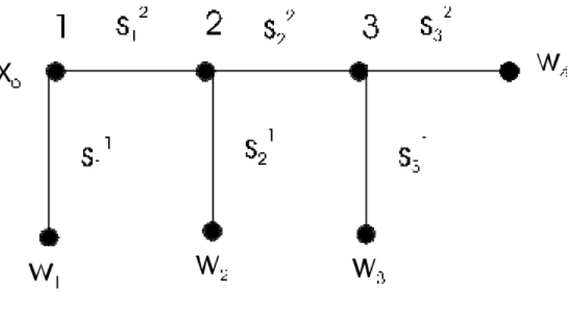
Figure 1: A three-player perfect information game

Hence, the replacing b

by b

is irrelevant to the incentives at reached decision points. In other words, U

¡ b

; b

j x ¢

¸ U

(b

; b

j x ) for all reached decision points x 2 X

and all b

2 B

, for i = 1; 2. Therefore, b

is a best reply against b

for i = 1; 2.

Since b

is a best reply against b

by hypothesis, under the assumption that there are only two players, linearity of the payo¤ function implies that b

is a best reply against ¸b

+ (1 ¡ ¸) b

for all ¸ 2 [0; 1], for i = 1; 2.

Interchanging the roles of b

and b

, an analogous argument shows that b

is a best reply against ¸b

+ (1 ¡ ¸) b

for all ¸ 2 [0; 1], for i = 1; 2.

But then, under the assumption of only two players, linearity of the payo¤

function implies that ¹b

+(1 ¡ ¹) b

is a best reply against ¸b

+(1 ¡ ¸) b

for all ¹ 2 [0; 1] and all ¸ 2 [0; 1], for i = 1; 2. In particular, ¸b

+ (1 ¡ ¸) b

2 C is a Nash equilibrium with outcome ¼

for all ¸ 2 [0; 1]. Thus, we have shown:

Proposition 1 For a …nite generic two-player perfect information extensive form game, every component of Nash equilibria is convex.

Unfortunately, this conclusion is peculiar to two-player perfect informa-

tion games. With more players only a weaker property holds: it will be

shown that, for a generic perfect information game, all components of Nash

equilibria are contractible.

But …rst, it is illustrated that convexity may fail for more than two players.

Example 1 Consider the three-player extensive form game in Figure 1, where

…rst player 1 can either terminate, yielding v (w

) = (5; 0; 0), or give the move to player 2. If player 2 is reached, she can terminate, yielding v (w

) = (0; 3; 3), or give the move to player 3. If player 3 is reached, she chooses be- tween payo¤ vectors v (w

) = (9; 1; 2) and v (w

) = (1; 2; 1). (The …rst entry in payo¤ vectors is player 1’s, the second player 2’s, and the third player 3’s payo¤.) This yields the following normal form.

s

s

s

s

5

0 0

5 0

0 0

3 3

9 1

2 s

s

s

s

s

5

0 0

5 0

0 0

3 3

1 2

1 s

The component C ¹ that contains the subgame perfect equilibrium (the “back- wards induction component”, henceforth) is given by ¾

(s

) = 1 and

1 ¸ ¾

¡ s

¢

¸ ¡ 8¾

¡ s

¢

¡ 4 ¢

= ¡

1 + 8¾

¡ s

¢¢

In the face ¾

(s

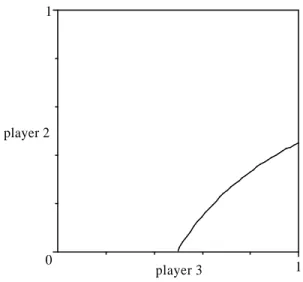
) = 1 of the cube £ (in which C ¹ is contained) this is depicted by all points to the northwest of the concave curve in Figure 2, where ¾

(s

) is on the horizontal and ¾

(s

) on the vertical axis. (The subgame perfect equilibrium is located at the point (1; 1) in Figure 2.) Therefore, C ¹ fails to be convex.

The example also illustrates another point. It is tempting to prove that at least the backwards induction component C ¹ is contractible by starting “at the end” and contracting behavior strategies towards subgame perfect behavior.

But, in the example, consider the equilibrium where player 1 terminates at the beginning, player 2 continues, and player 3 chooses v (w

) = (1; 2; 1) (point (0 ; 0) in Figure 2), rather than v (w

) = (9; 1; 2), as in the subgame

2A subset of a Euclidean space iscontractible if the identity is homotopic to a constant.

0 1

player 2

player 3 1

Figure 2: The backwards induction component is not convex

perfect equilibrium. This is an equilibrium in C ¹ , because players 2 and 3 are not reached and their behavior does not induce 1 to deviate. Yet, if player 3’s choice at her (…nal) decision point is switched to subgame perfect equilibrium behavior (keeping strategies of other players …xed), the resulting strategy combination is not an equilibrium. (It corresponds to the bottom- right point (1; 0) in Figure 2.)

Therefore, and because the argument will apply to all components, the focus cannot be on subgame perfect behavior. Rather, for a component C with associated outcome ¼ (constant across the component), consider the strategy combination obtained by working backwards in the tree, and mod- ifying the behavior of agents at unreached nodes to minimize the payo¤ of the last player who is reached along the path to this node. (Note that if x and y are two unreached nodes along the same path, the “last player” is the same, and so there is no inconsistency in this construction.) Iteratively modifying all strategies towards this strategy combination preserves equilib- rium and the outcome ¼ and, thus, remains inside the component C. This modi…cation results in a homotopy between the identity on C and a constant function that maps into a particular strategy combination.

In the example, the relevant player at both unreached nodes is player 1,

and the actions that minimize 1’s payo¤ are s

and s

: Following this order, all

strategy combinations in Figure 2 are …rst moved horizontally to the left edge of the square, and then vertically up to the top left corner. Note that in this example, even though the component in question was the backward induction one, the resultant strategy combination is not the backward induction one.

However, it is, of course, the case that if a set can be contracted to one point in itself, then it can also be contracted to any other, and so for backward induction components, the contraction toward the non-backward induction outcome is only for technical convenience.

Theorem 1 For a …nite generic perfect information extensive form game, every connected component of Nash equilibria in behavior strategies is con- tractible.

Proof. Fix a generic perfect information extensive form game and order decision points as follows. De…ne X

as the union of chance moves X

with all terminal nodes and for any t = 1; 2; ::: de…ne X

recursively as the set

© x 2 X

¯¯ if x comes before y 2 N n f x g , then y 2 [

X

ª (6) That is, X

contains all decision points which come before terminal nodes or chance moves only; from moves in X

only terminal nodes, chance moves, or moves in X

can be reached, and so forth.

Now, consider a particular component C µ B of Nash equilibria and let ¼

denote the unique outcome associated with equilibria in C. A move x 2 X is reached if ¼

(x) = P

x2w

¼

(w) > 0, otherwise it is unreached (see (4)).

Because the game is …nite, for any unreached decision point x 2 X

there is a unique smallest t (x) = 1; 2; ::: such that ¼

¡ P

(x) ¢

> 0: Denote this by » (x) = P

(x) and let ¶ (x) 2 f 1; :::; n g be the player such that

» (x) 2 X

. That is, »(x) is the last node reached on the path to x; and

¶ (x) is the player to whom »(x) belongs. Note that ¶ (x) must be a personal player, because » (x) 2 X

would imply ¼

(y) > 0 for all y 2 P

(» (x)) in contradiction to the construction of » (x). If x 2 X

is unreached, then

¼

(y) = 0 for all y 2 N that come (properly) after » (x).

We de…ne now a recursive procedure for how to modify a given equilibrium

b 2 C. Consider any b = b

2 C and an unreached decision point x 2 X

.

Assume that behavior at all decision points (of personal players) that come

after x has been adjusted to b

in accordance with the procedure, where

b

2 C is an equilibrium with outcome ¼

. (If t = 1 this assumption is

void, providing a starting point for the recursive procedure.) Let i be such that x 2 X

and choose a successor y 2 P

(x) such that

U

¡ b

j y ¢

· U

¡ b

j z ¢

for all z 2 P

(x)

Then, modify i’s behavior at x such that y 2 P

(x) is chosen with certainty and denote the resulting behavior strategy combination by b

= ¡

b

; b

¢ B. (That is, b

is identical to b

, except possibly at x.) 2

We claim that ¸b

+(1 ¡ ¸) b

2 C for all ¸ 2 [0; 1]: First, since behavior under b

di¤ers from that under b

only at the unreached move x, both b

and b

must induce the same outcome, ¼

. Next, by the construction of b

; for any unreached move y 2 X

player ¶ (y) cannot gain more by deviating at » (y) under b

than she could have gained under b

: Therefore, if b

is an equilibrium, so is b

. Moreover, for any unreached move y 2 X

player

¶ (y)’s conditional payo¤ U

(¸b

+ (1 ¡ ¸) b

j » (y)) is linearly increasing (or constant) in ¸, implying that ¸b

+ (1 ¡ ¸) b

2 C for all ¸ 2 [0; 1], as desired.

Repeat this modi…cation for all x 2 X

to obtain b

2 C. Since each x 2 X

is the root of a separate subgame (by the perfect information assumption), all these modi…cations can be done independently.

Now, let ¿ 2 f 1; 2; ::: g be the maximum over unreached decision points x 2 X

such that P

(x) = » (x). We de…ne for every t = 1; :::; ¿ recursively a continuous function h

: C £ [0; 1] ! C such that h

(b; 0) = b for all b 2 C . For t = ¿ this will yield the desired homotopy.

De…ne h

: C £ [0; 1] ! C as the identity, h

(b; ¸) = b for all b 2 C and all ¸ 2 [0; 1]. For t > 0, enumerate by x

; :::; x

all unreached moves in X

, denote by j(m) the player for whom x

2 X

\ X

, let b

(b) = h

(b; 1), and de…ne recursively

b

(b) = ³

b

(b) ; b

´

for all m = 1; :::; k

where b

is constructed as above. Then, de…ne for every t = 1; :::; ¿ re- cursively the functions h

: C £ [0; 1] ! C by h

(b; ¸) = h

(b; 2¸) for all

¸ 2 [0; 1 =2] and

h

(b; ¸) = (2k¸ ¡ k ¡ m + 1) b

(b) + (k + m ¡ 2k¸) b

(b)

for all ¸ 2 ((k + m ¡ 1) =2k; (k + m) =2k] and all m = 1; :::; k.

Choosing t = ¿ , a continuous piecewise linear function h

: C £ [0; 1] ! C is obtained such that h

(b; 0) = b for all b 2 C and under h

(b; 1) for any unreached move x 2 [

X

the conditional payo¤ of player ¶ (x) given

» (x) is minimized with respect to behavior at x. Since h

(b; 1) does not depend on b, the desired homotopy has been constructed.

Since mixed strategies of the normal form induce behavior at all decision points (see Appendix), the logic of the proof carries over to mixed strategies as well.

Corollary 1 For a …nite generic perfect information extensive form game, every connected component of Nash equilibria in mixed strategies is con- tractible, both in the normal form and the reduced normal form.

Proof. For the reduced normal form the statement follows from Proposition 2 in the Appendix. For the (unreduced) normal form, the proof is identical to the one of Theorem 1, except that any given mixed equilibrium ¾ =

¾

2 C µ £, for an unreached decision point x 2 X

\ X

and a node y 2 arg min

U

(¾

j z ), is modi…ed as follows.

De…ne S

(y) = f s

2 S

j s

(x) = y g as the set of i’s pure strategies that choose y at x, the mapping '

: S

! S

(y) by '

(s

) (z) = s

(z) for all z 2 X

n f x g , and let ¾

2 ¢

be the unique mixed strategy that satis…es

¾

(s

) = X

ri2'^¡1_x (si)

¾

(r

) for all s

2 S

(y)

Then the behavior induced by ¾

agrees with the one induced by ¾

at all reached (according to ¼

) moves of i.

Therefore, ¾ 2 C and ¾

= (¾

; ¾

) 2

£ induce the same outcome (¼

). Moreover, player ¶ (x) cannot gain more by deviating at » (x) under ¾

than she could have gained under ¾, by the construction of ¾

. Hence, if ¾ is an equilibrium, so is ¾

. Linearity of the payo¤ function in ¾

then implies that ¸¾ + (1 ¡ ¸) ¾

is an equilibrium for all ¸ 2 [0; 1]. Since C is connected, it follows that ¸¾ + (1 ¡ ¸) ¾

2 C for all ¸ 2 [0; 1].

Consequently, ¾

can play the same role as b

in the proof of Theorem 1, and the homotopy can be constructed analogously.

3In fact, the behavior induced by¾^x_i agrees with the one induced by¾iat all moves ofi that can be reached under both strategies (each combined with some strategy combination among the opponents), with the possible exception ofx.

As pointed out earlier, this result has important applications in evolu- tionary game theory. It implies that, if evolution selects any equilibrium component at all (by asymptotic stability in a selection dynamics), then for generic perfect information games it will be the backwards induction com- ponent (Demichelis and Ritzberger (2000), Theorem 1). This is, because the backwards induction component is the only one for which its index agrees with its Euler characteristic.

This, of course, does not imply that there is always a sensible selection dynamics for which the backwards induction component is asymptotically stable. In fact, Cressman and Schlag (1998) give an example of a perfect information game for which the backwards induction component cannot be asymptotically stable in the replicator dynamics. Since this is a game where each player has only two strategies, it is easy to show that the backwards induction component cannot be asymptotically stable in any “payo¤ consis- tent” (for a de…nition see Demichelis and Ritzberger (2000)) selection dy- namics either.

Still, Theorem 1 shows that for perfect information games the situation is better than for two-player outside option games (van Damme (1989), Hauk and Hurkens (forthcoming)). In the latter class there are games which have no component for which the index agrees with the Euler characteristic. So, the present insight represents at least some support for backwards induction.

The preceding result has an additional interesting implication. The ho- motopy from Theorem 1 yields pure choices at unreached moves. Since at reached moves a backwards induction argument shows that generically all choices are pure, it follows that the constant strategy combination h

( : ; 1) is a pure strategy combination s 2 C which is such that the incentives for agents at the equilibrium path to deviate into unreached subgames are min- imized. This demonstrates the following.

Corollary 2 For almost all …nite perfect information extensive form games, every component of Nash equilibria contains a pure strategy combination.

Topologically Theorem 1 says that the equilibrium set of a generic perfect

information game is equivalent to a …nite collection of points, both in mixed

and behavior strategies. Precisely one of these corresponds to the (unique)

subgame perfect equilibrium.

4 Subgame Perfect Equilibria

Perfect information games constitute the prime case where subgame perfect equilibrium appears to be the natural equilibrium re…nement concept. This is so because such games have the highest possible degree of decomposability.

Ever player, when called upon to move, knows the entire history that led to her move, there are no simultaneous decisions, and every choice leads into a subgame. This makes perfect information game the ideal domain for backwards induction. Accordingly, we now turn to the set of subgame perfect equilibria for perfect information games.

First, it is well known that in generic perfect information games the sub- game perfect equilibrium is unique (in behavior strategies). So, the inter- esting cases are degenerate perfect information games. But for those, the conclusion from Theorem 1 on Nash equilibrium components fails, as the following example shows.

Example 2 Consider again the three-player perfect information game from Figure 1, but now with the degenerate payo¤ function v (w

) = (0; 0; 0), v (w

) = (0; 0; 0), v (w

) = (2; ¡ 1; 0), and v (w

) = ( ¡ 1; 2; 0). (Player 3’s payo¤s at w

and w

do not matter for the argument.) In this game player 3 is always indi¤erent when she is called upon to move. Yet, depending on what player 3 chooses, the other players will want to either take their outside op- tions (s

for i = 1; 2) or to pass the move on (s

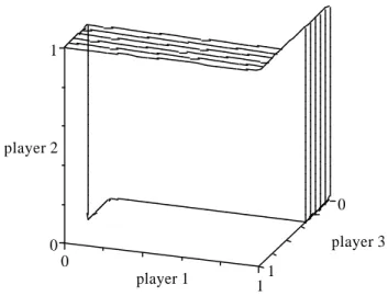
for i = 1; 2). The set of Nash equilibria consists of a single connected component that is homeomorphic to a circle with two rectangles glued to it, and hence, is homotopy-equivalent to a circle. It is given by the union of

the segment ¾

¡ s

¢

= 1, 0 · ¾

¡ s

¢

· 1, ¾

¡ s

¢

= 2=3, the rectangle 0 · ¾

¡ s

¢

· 1, ¾

¡ s

¢

= 1, 2=3 · ¾

¡ s

¢

· 1, the segment ¾

¡

s

¢

= ¾

¡

s

¢ = 1, 1=3 · ¾

¡ s

¢

· 2=3, the rectangle ¾

¡

s

¢

= 1, 0 · ¾

¡ s

¢

· 1, 0 · ¾

¡ s

¢

· 1=3, the segment 0 · ¾

¡

s

¢

· 1, ¾

¡ s

¢

= 1, ¾

¡ s

¢

= 1=3, and the segment ¾

¡ s

¢

= ¾

¡ s

¢

= 1, 1=3 · ¾

¡ s

¢

· 2=3.

Hence, the only component of Nash equilibria in this game is not contractible.

Figure 3 illustrates with ¾

(s

) on the horizontal axis, ¾

(s

) on the vertical

axis, and ¾

(s

) on the third axis.

0

1

player 3 0

player 1 1 0

1

player 2

Figure 3: The set of Nash equilibria is homotopy-equivalent to a circle But not all the Nash equilibria of this game are subgame perfect. More precisely, all Nash equilibria belonging to the segment (third piece), ¾

(s

) =

¾

(s

) = 1, 1=3 · ¾

(s

) · 2=3, and the rectangle (fourth piece), ¾

(s

) = 1, 0 · ¾

(s

) · 1, 0 · ¾

(s

) · 1=3, (the rightward “vertical” rectangle and the upper line segment connecting it to the other rectangle, in Figure 3) fail subgame perfection. (All other equilibria are subgame perfect.) Therefore, if only those Nash equilibria, whose outcome corresponds to a subgame perfect equilibrium, are considered, these do form a contractible component.

The example suggests that, for degenerate perfect information games, the set of Nash equilibria may have a complicated structure. Yet, the set of subgame perfect equilibria appears to be simpler. Theorem 2 below shows that this is indeed so. Intuitively, it says that the set of subgame perfect equilibria “has no holes”, even for degenerate perfect information games.

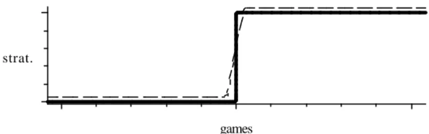
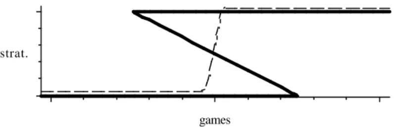
Theorem 3 extends this observation to a statement about the graph of

the subgame perfect equilibrium correspondence (from perfect information

games with a …xed tree to, say, behavior strategies). It says that an arbitrary

small perturbation makes the graph of this correspondence into the graph of

a (continuous) function. Figure 4 illustrates this: The bold graph depicts

the correspondence mapping perfect information games (on the horizontal

strat.

games

Figure 4: Perturbing the subgame perfect equilibrium correspondence axis) into subgame perfect equilibria (i.e. strategies on the vertical axis); the broken graph depicts an appropriate small perturbation.

Before stating the theorems, however, it has to be clari…ed what “sub- game perfect” means for mixed strategies. For the (unreduced) normal form, subgame perfect equilibria are well de…ned, provided an extension of Bayes’

rule is adopted for decision points that are not reached (see Appendix). Such an extension, however, cannot be continuous.

For the reduced normal form mixed strategies only induce behavior at de- cision points that can be reached - but they do so continuously. Thus, for the reduced normal form subgame perfection has to be de…ned more loosely. Ac- cordingly, de…ne a mixed equilibrium of the (mixed extension of the) reduced normal form as subgame perfect if its image in behavior strategies contains a subgame perfect equilibrium (see Appendix). Since behavior strategies map continuously into mixed strategies (both for the normal form and the reduced normal form; see Lemma 2 in the Appendix), we continue to work with behavior strategies.

Fix an extensive form with perfect information F with n players. Let B = £

B

be the associated space of behavior strategy combinations and identify the set of all payo¤ functions v : W ! R

with a Euclidean space R

of appropriate dimension, i.e. with K = n j W j . The latter is then the space of all perfect information games with extensive form F . The subgame perfect equilibrium correspondence E : R

! B maps each perfect information game G = (F; v) into the set E (v) of its subgame perfect equilibria (in behavior strategies). Denote by G = ©

(v; b) 2 R

£ B j b 2 E (v) ª

the graph of the

subgame perfect equilibrium correspondence.

For most of the space of perfect information games E is a function. At degenerate games the structure of E (v) is yet unknown. The next result clari…es the geometry of E (v) for all perfect information games.

Theorem 2 For every perfect information extensive form game the set E (v) of subgame perfect equilibria is contractible.

Proof. For a given extensive form F denote by ¿ (F ) ¸ 1 the unique integer such that X = [

X

. We proceed by induction over the “size” ¿ (F ) of the tree. If ¿ (F ) = 1, then all moves come before terminal nodes or chance moves only; hence, there is only a single player, who decides once and for all at the root. The set E (v) is then the convex hull of this player’s choices, that maximize the single player’s expected payo¤, and, therefore, a contractible polyhedron.

Now, suppose the statement of the proposition holds true for all ¿ (F ) = 1; :::; k ¡ 1 and consider an extensive form F for which ¿ (F ) = k. Let i be the player, who decides …rst (at the root). Each of player i’s choices leads to the root of a subgame G

= (F

; v

) with x 2 P

(x

) for which

¿ (F

) is at most k ¡ 1 (where v

denotes the restriction of v to the plays passing through x 2 X). Hence, by the induction hypothesis, the set of subgame perfect equilibria of each of the subgames G

with x 2 P

(x

) is contractible and polyhedral (in fact, a simplex).

Consider the map Á from E (v) into the product £

E (v

) of sub- game perfect equilibria of subgames starting immediately after the (decision at the) root that assigns to each subgame perfect equilibrium of G the equi- libria that it induces in the subgames G

with x 2 P

(x

). Since the game is …nite, this map is surjective, because every (subgame perfect) equilibrium of a subgame G

is part of a subgame perfect equilibrium of G by Kuhn’s Lemma (Kuhn (1953)).

Now consider the preimage Á

(b) of a point

b = (b

)

2 £

E (v

)

where b

denotes an equilibrium of the subgame G

for all x 2 P

(x

). This

preimage is nonempty, because the map is surjective. Since the behavior

strategy combination b assigns a unique probability distribution to each set

of plays passing through a move x 2 P

(x

), every such move is associated

with a unique expected payo¤ for player i. Therefore, the preimage Á

(b) is

the face (subsimplex) of player i’s behaviors simplex spanned by the choices at the root, that assign payo¤ maximizing choices at the root, and behavior consistent with b in later parts of the tree, together with b. It follows that Á

(b) is contractible (in fact, convex).

In other words, Á is a surjection for which the preimage of any point is contractible. Since, by the induction hypothesis, each E (v

) is also polyhe- dral, Á is a cell-like map (for a de…nition see Lacher (1969), p. 718). For cell-like maps on polyhedra Corollary 1.3 of Lacher ((1969), p. 720) implies that the map is a homotopy equivalence.

It follows that the whole set E (v) is contractible also for ¿ (F ) = k.

The proof of Theorem 2 could have been stated for mixed strategies of the normal form without changing the argument. This observation together with Proposition 2 (in the Appendix) yields the following.

Corollary 3 For every perfect information extensive form game, the set of subgame perfect equilibria is contractible, both in the normal form and the reduced normal form.

Furthermore, since every contractible set is connected, a perfect informa- tion game cannot have two distinct components of Nash equilibria both of which contain subgame perfect equilibria. Again, this also holds for all types of strategies.

Corollary 4 Every perfect information extensive form game has precisely one connected component of subgame perfect equilibria, both in behavior and mixed strategies.

At this point we know two things: First, on an open dense subset of R

the correspondence E is a function. Second, at nongeneric points, where it is not, E (v) is a contractible set. If the branches of E over generic v’s hang nicely together by contractible pieces, then there is a good chance that the whole graph G “looks like” the space R

of games, at least after some mild deformation. And, indeed, a slight modi…cation of the mapping used by Kohlberg and Mertens (1986) serves to show precisely this.

As a …rst step, we characterize the mapping introduced by Kohlberg and Mertens (1986) in a geometrically transparent way.

4We are grateful to Steve Ferry for providing the adequate reference.

Lemma 1 Let ® : R

! ¢

be de…ned by ® (v) = arg min

k v ¡ a k , where ¢

denotes the (l ¡ 1)-dimensional unit simplex, for some integer l ¸ 1. Then:

(a) ® is a continuous function such that a = ® (v) is the unique …xed point of the mapping f

: ¢

! ¢

de…ned by

f

(b) = arg max

a2¢^l¡1

a ¢ (v ¡ b) , for all v 2 R

(b) if u = v + re 2 R

for some r 2 R with e = (1; 1; :::; 1) 2 R

, then

® (u) = ® (v).

Proof. First, note that k v ¡ a k is minimized at a 2 ¢

if and only if

¡ k v ¡ a k

is maximized at a 2 ¢

. Since for all a; b 2 ¢

and all

¸ 2 (0; 1)

k v ¡ ¸a ¡ (1 ¡ ¸) b k

· ¸ k v ¡ a k

+ (1 ¡ ¸) k v ¡ b k

where equality implies a = b, that ¢

is convex implies that ® (v) is unique for all v 2 R

. Hence, ® is a function that is continuous by the maximum theorem (that yields upper hemi-continuity).

(a) That f

has a …xed point, follows from Kakutani’s …xed point theorem by observing that f

(b) is a face of ¢

(and, therefore, convex) for all b 2

¢

and applying the maximum theorem (to deduce upper hemi-continuity).

To see that b 2 f

(b) if and only if b = ® (v), let b 2 ¢

and a = ® (v).

By de…nition,

k v ¡ b k

¸ k v ¡ a k

= k v ¡ b k

+ 2 (b ¡ a) ¢ (v ¡ b) + k b ¡ a k

(7) , k b ¡ a k

· 2a ¢ (v ¡ b) ¡ 2b ¢ (v ¡ b) (8) Therefore, if b 2 f

(b) and there is some a 2 ¢

such that k v ¡ a k <

k v ¡ b k , then inequality (7) would be strict, so that b ¢ (v ¡ b) = max

c2¢^l¡1

c ¢ (v ¡ b) ¸ a ¢ (v ¡ b) (9) would imply the contradiction k b ¡ a k < 0 by (8). Hence, b 2 f

(b) implies b = ® (v). Conversely, if b 2 f

(b) and a = ® (v), then (9) implies from (8) that k b ¡ a k

· 0, i.e. b = a. Because ® is a function, the …xed point of f

is unique for all v 2 R

.