Frictional effects, vortex spin-down
To understand spin-up of a tropical cyclone it is instructive to consider first the spin-down problem, which requires a consideration of frictional effects. We examine first the essential dynamics of the problem and proceed then to a scale analysis of the equations with the friction terms included.
4.1 Spin-down of a rotating vortex
The classic vortex spin down problem considers the evolution of an axisymmetric vortex above a rigid boundary normal to the axis of rotation. We will show that the spin down is intimately connected to the Coriolis torques associated with the secondary circulation induced by friction. The direct effect of the frictional diffusion of momentum to the surface is of secondary importance in the parameter regimes relevant to tropical cyclones.
In a shallow layer of air near the surface, typically 500 - 1000 m deep, frictional stresses reduce the tangential wind speed and thereby the centrifugal and Coriolis forces, while it can be shown that the force associated with the radial increase of pressure remains largely unchanged. We call this layer the friction layer. The result of the force imbalance is a net inward force that drives air parcels inwards in this layer. One can demonstrate this effect by placing tea leaves in a beaker of water and vigorously stirring the water to set it in rotation. After a short time the tea leaves congregate near the bottom of the beaker near the axis as shown in Fig. 4.1:
they are swept there by the inflow in the friction layer. Slowly the rotation in the beaker declines because the inflow towards the rotation axis in the friction layer is accompanied by radially-outward motion above this layer. The depth of the friction layer depends on the viscosity of the water and the rotation rate and is typically only on the order of a millimetre or two in this experiment. Because the water is rotating about the vertical axis, it possess angular momentum about this axis. Here angular momentum is defined as the product of the tangential flow speed and the radius. As water particles move outwards above the friction layer, they conserve their angular momentum and as they move to larger radii, they spin more slowly.
81
Figure 4.1: The beaker experiment showing the effects of frictionally-induced inflow near the bottom after the water has been stirred to produce rotation. This inflow carries tea leaves to form a neat pile near the axis of rotation.
The same process would lead to the decay of a hurricane if the frictionally-induced outflow were to occur just above the friction layer, as in the beaker experiment.
What then prevents the hurricane from spinning down, or, for that matter, what enables it to spin up in the first place? Clearly, if it is to intensify, there must be a mechanism capable of drawing air inwards above the friction layer, and of course, this air must be rotating about the vertical axis and possess angular momentum so that as it converges towards the axis it spins faster. The only conceivable mechanism for producing inflow above the friction layer is the upward ”buoyancy force” in the clouds, the origins of which we examine below.
4.2 Scale analysis of the equations with friction
We repeat now the scale analysis of the dynamical equations (3.1) - (3.3) with the friction terms K(∇2u,∇2v,∇2w) added to the right-hand-sides. We have assumed a particularly simple form for friction with K an eddy diffusivity, assumed to be con- stant. We assume that the air is homogeneous and that the motion is axisymmetric and define velocity scales (U, V, W), length scales (R, Z), and an advective time scale T = U/R as before. Now we assume that p is perturbation pressure and take Δp to be a scale for changes in this quantity. The continuity equation, (3.4), yields the same relation between W/Z ∼U/Ras before. Then the terms in Eqs. (3.1) to (3.3) have nondimensional scales as shown in Table 4.1.
As in section 3.5 we divide terms in line (2a) by V2/R to obtain those in line (2b) and divide terms in line (3a) by U V /R to obtain those in line (3b). The
terms in line (4a) are divided by g to obtain those in line (4b). The terms in lines (b) are then nondimensional. We define a Reynolds number, Re = V Z/K, which is a nondimensional parameter that characterizes the importance of the inertial to frictional terms, and an aspect ratio A = Z/R, that measures the ratio of the boundary-layer depth to the radial scale.
u-momentum
∂u
∂t +u∂u
∂r +w∂u
∂z −v2
r −f v = −1 ρ
∂p
∂r +K
∇2hu− u r2
+K∂2u
∂z2 (4.1) U
T
U2
R WU
Z
V2
R f V Δp
ρR K U
R2 K U
Z2 (1a)
S2 S2 S2 1 1
Ro
Δp
ρV2 SA2R−1e SR−1e (1b) v-momentum
∂v
∂t +u∂v
∂r +w∂v
∂z +uv
r +f u = +K
∇2hv− v r2
+K∂2v
∂z2 (4.2) V
T UV
R WV
Z UV
R f U K V
R2 K V
Z2 (2a)
S S S S S
Ro A2R−1e R−1e (2b)
w-momentum
∂w
∂t +u∂w
∂r +w∂w
∂z = −1
ρ
∂p
∂z +K∇2hw +K∂2w
∂z2 (4.3)
W T
U W R
W W Z
Δp
ρZ KW
R2 KW
Z2 (3a)
S2A2 S2A2 S2A2 Δp
ρV2 SA3R−1e SAR−1e (3b) Table 4.1: Scaling of the terms in Eqs. (3.1) to (3.3) with frictional terms added.
Here ∇2h = (∂/∂r)(r∂/∂r).
Typically, the boundary layer is thin, not more than 500 m to 1 km in depth and the aspect ratio is small compared with unity. Moreover, typical values of K are on the order of 10 m s−2. Therefore takingV = 50 m s−1,R = 50 km, andZ = 500 m,
Re= 2.5×10³ and A= 10−2. It follows from line (3b) in Table 4.1 that Δp/(ρV2)≈ max(S2A2,SAR−1e ) = 4×10⁻⁴, assuming thatS ≈1 in the boundary layer. Thus the vertical variation of p across the boundary layer is only a tiny fraction of the radial variation of p above the boundary layer. In other words, to a close approximation, the radial pressure gradient within the boundary layer is the same as that above the boundary layer.
From lines (1a) and (2a) in Table 4.1, we see that a vertical scaleZ which makes friction important compared with the other large terms is (K/f)12 if Ro <<1 and (K/(V /R))12 if Ro ≈1 or larger. The former result gives us the appropriate scaling for the Ekman layer.
4.3 The Ekman boundary layer
The scale analysis of the u- and v-momentum equations in Table 4.1 show that for small Rossby numbers (Ro <<1), there is an approximate balance between the net Coriolis force and the diffusion of momentum, expressed by the equations:
f(vg−v) =K∂2u
∂z2 (4.1)
and
f u=K∂2v
∂z2, (4.2)
where we have used the fact deduced from the scale analysis of the w-momentum equation that the horizontal pressure gradient in the boundary layer is essentially the same as that above it. Thus we have replaced the radial pressure gradient in Eq.
(4.1) by the geostrophic wind, vg, above the boundary layer. We assume also that the radial flow above the boundary layer is zero.
Equations (4.1) and (4.2) are linear in u and v and may be readily solved by setting V = v+iu, where i = √
(−1). Then they reduce to the single differential equation
Kd2V
dz2 −if V =−if Vg, (4.3)
where Vg = vg. This equation has the particular integral V =Vg and there are two complementary functions proportional to exp(±(1−i)z/δ), whereδ =√
2K/f. Since we require a solution that remains bounded as z → ∞we reject the solution with a positive exponent so that the solution has the form
V =Vg[1−Aexp(−(1−i)z/δ),] (4.4) whereAis a complex constant determined by a suitable boundary condition atz = 0.
For a laminar viscous flow, the flow atz= 0 is zero givingA= 1. This is the classical Ekman solution. The profiles of u and v are shown in Fig. 4.2a and the hodograph thereof is the Ekman spiral shown in Fig. 4.2b. Two interesting features of the
solution are the fact that the boundary-layer thickness, measured by δ is a constant and there are regions in the boundary layer where the flow is supergeostrophic, i.e. v > Vg. These are unusual features of boundary layers which are typically regions where the flow is retarded and which grow in thickness downstream as more and more fluid is retarded. In the Ekman layer, the fluid that is retarded in the downstream direction, but is re-energized in the cross-stream direction by the net pressure gradient force in that direction. The latter occurs because friction reduces the Coriolis force in the boundary layer whereas the radial pressure gradient remains effectively unchanged. The height range where the flow is supergeostrophic is one in which the net radial flow is outwards. The fact that the radial flow is inwards over this range is a result of the upward diffusion of u-momentum, which is largest at low levels.
The existence of a region of supergeostrophic winds may be made plausible by considering the spin-down problem in which there is initially a uniform geostrophic flow, Vg, at large radius. If the frictional stress is switched on at the surface at time zero, the tangential flow will be reduced near the surface leading to a net pressure gradient in the radial direction. This will drive a radial flow that is largest near the surface where the net pressure gradient is largest. The Coriolis force acting on the radial flow will tend to accelerate the tangential flow as part of an inertial oscillation.
Whether or not the tangential flow becomes supergeostrophic after some time will depend subtly on the vertical diffusion of momentum in the radial and tangential directions, but the Ekman solution indicates that it does.
The classical Ekman solution with a no-slip boundary condition at the surface is a poor approximation in the atmospheric boundary layer. A better one is to prescribe the surface stress, τ0, as a function of the near-surface wind speed, normally taken to be the wind speed at a height of 10 m, and a drag coefficient, CD. The condition takes the form
τ0
ρ =K∂V
∂z =CD|V|V (4.5)
and we shall apply it at z = 0 instead of 10 m. Substituting (4.4) into (4.10) and tidying up the equation gives
(1−i)A=ν|1−A|(1−A) (4.6) where ν = CDRe and Re = Vgδ/K is a Reynolds’ number to the boundary layer.
Setting 1−A=Beiβ gives after a little algebra an equation forB and an expression for β in terms of B (see Exercise 4.1). The equation for B may be solved using a Newton-Rapheson algorithm. Profiles of u(z) and v(z) obtained for values Vg = 10 m s−1,f = 10−4 s−1,K = 10 m2 s−2 andCD = 0.002 are shown in Fig. 4.2a also and the corresponding hodograph is shown in Fig. 4.2b. For these values, the boundary layer depth scale, δ = 450 m and the surface values of v and u are about 0.7Vg and 0.2Vg, respectively.
(a)
(b)
Figure 4.2: (a) Vertical profiles of tangential and radial wind components for the Ekman layer (red curves) and the modified Ekman layer based on a surface drag formulation (blue curves). (b)Hodograph of the two solutions showing the spiral of the wind vector.
4.4 The modified Ekman layer
From the scale analysis in Table 4.1, the full u−and v−momentum equations in the boundary layer are:
∂u
∂t +u∂u
∂r +w∂u
∂z +V2−v2
r +f(V −v) =K∂2u
∂z2, (4.7)
∂v
∂t +u∂v
∂r +w∂v
∂z +uv
r +f u=K∂2v
∂z2, (4.8)
where V(r) is the gradient wind speed above the boundary layer. With the substi- tution v =V(r) +v, these equations become:
∂u
∂t +u∂u
∂r +w∂u
∂z − v2 r −
2V r +f
v =K∂2u
∂z2 (4.9)
∂v
∂t +u∂v
∂r +w∂v
∂z + uv r +
dV dr +V
r +f
u=K∂2v
∂z2 (4.10)
We carry out now a scaling of the terms in these equations as shown in Table 4.2.
Let U, V∗ and V be scales for u, V and v, respectively. Examination of the u- and v-profiles for the case with a surface drag coefficient in Fig. 4.2 suggests that U ≈V ≈0.2V∗−0.3V∗. Accordingly we assume thatU =Vand defineS∗ =U/V∗, which may be as large as 0.3.
u-momentum
∂u
∂t +u∂u
∂r +w∂u
∂z −v2
r −
2V r +f
v = +K∂2u
∂z2 (4.9) U
T
U2
R WU
Z
V2 R
2V∗V
R f V K U
Z2 (1a)
S∗ S∗ S∗ S∗ 2 1
Ro Re−1R
Z (1b) v-momentum
∂v
∂t +u∂v
∂r +w∂v
∂z +uv
r +
∂V
∂r + V r +f
u = +K∂2v
∂z2 (4.10) V
T UV
R WV Z
U V R
V U R
V U
R f U KV
Z2 (2a)
S∗ S∗ S∗ S∗ 1 1 1
Ro Re−1R
Z (2b) Table 4.2: Scaling of the terms in Eqs. (4.9) to (4.10). Here S∗ =U/V∗ =V/V∗, Ro=V∗/(f R) and Re=V Z/K.
With the background gradient wind balance removed, there is less of a scale sep- aration between the various terms in the boundary-layer equations. If ζ∗ is regarded
as small compared with unity, we could linearize Eqs. (4.9) and (4.9) to obtain
− 2V
r +f
v =K∂2u
∂z2, (4.11)
dV dr + V
r
u=K∂2v
∂z2. (4.12)
It is interesting to examine this approximation even though the neglect of terms of magnitude 0.2-0.3 compared with unity is unlikely to be very accurate. For one thing the equations (4.11) and (4.12) are relatively easy to solve and thy are a generalization of the Ekman layer theory derived in the previous subsection. The difference in the coefficients of v and u on the left-hand-side of the equations precludes the method used for the Ekman equations (4.1) and (4.2). Now we differentiate one of the equations twice with respect to z and use the remaining equation to eliminate either u or v. Then each of these quantities satisfies the equation
∂4x
∂z4 +I2x
K2 = 0 (4.13)
The solutions have the formx=aeαz whereα4 = (I2/K2)eiπ+2nπi, (n = 0, 1, 2, 3), and a is a constant. Thus the four roots are α=±(1±i)/δ, where δ= (2K/I)1/2 is the boundary-layer scale thickness. The solutions forv anduwhich decay asz → ∞ can be written succinctly in matrix form
v u
=V e−z/δ
a1 a2 b1 b2
cosz/δ sinz/δ
(4.14) where a1, a2, b1, b2 are constants. Two relations between these constants may be determined by applying the boundary condition (4.5), remembering that this applies to the total surface wind field (V +v, u). Two further relationships may be obtained by substituting for v and u in Eq. (4.12). The details form the basis of Exercise (4.2). Given a radial profile of V(r) such as that shown in Fig. 4.3, it is possible to calculate the full boundary-layer solution (u(r, z), v(r, z), w(r, z)) on the basis of Eq. (4.14). The vertical velocity, w(r, z) is obtained by integrating the continuity equation (see Exercise 4.3).
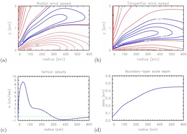
Figure 4.4 shows the isotachs ofuandv and the vertical velocity at the top of the boundary layer for the tangential wind profile shown in Fig. 4.3. It shows also the radial variation of the boundary layer depth scale,δ. Note thatδdecreases markedly with decreasing radius, while the inflow increases. The maximum inflow occurs in this case at a radius of 90 km, 50 km outside the radius of maximum wind speed above the boundary layer, rm. In contrast, the maximum vertical velocity at ”large heights” peaks just outside rm. There is a region of weak outflow above the inflow layer coinciding roughly with the region where tangential flow becomes subgradient.
Figure 4.3: Tangential wind profile as a function of radius used in the calculations for Fig. 4.4.
(a) (b)
(c) (d)
Figure 4.4: Isotachs of (a) radial wind, and (b) tangential wind in the r−z plane obtained by solving Eqs. (4.11) and (4.12) with the tangential wind profile shown in Fig. 4.4. (c) Vertical velocity at the top of the boundary layer, and (d) radial variation of boundary-layer scale depth, δ(r).
Exercise 4.1
Show that the substitution A= 1−Beiβ in eq (4.6) leads to the equation (νB+ 1)2+ 1 B2
(νB+ 1)2+ 1
−2
= 0 and the β is given by
tanβ=− νB νB+ 1
[Hint: after substitution, equate real and imaginary parts to obtain a pair of simultaneous equations for cosβ and sinβ.]
Exercise 4.2
Show that the substitution (4.14) into the boundary condition (4.5) gives the two relationships
a2−a1 =ν
(1 +a1) +b2112
(1 +a1), and
b2−b1 =ν
(1 +a1) +b2112 b1
and that the substitution into Eq. (4.12) gives two more relationships b1 =−2K
ξaδ2a2 and b2 = 2K ξaδ2a1,
where ξa = ζ + f. Show the points (a1, a2) lie on a circle centred at the point (−12,−12) with radius
1 V2 and may be expressed as a
a1 = 1
V2cosθ−1 2 ,
a2 = 1
V2sinθ− 1 2. Hence derive an equation for θ.
abc