The fault plane as the main fluid pathway: Geothermal field development options under subsurface and operational uncertainty

Research Collection

Journal Article

The fault plane as the main fluid pathway: Geothermal field development options under subsurface and operational uncertainty

Author(s):

Daniilidis, Alexandros; Saeid, Sanaz; Gholizadeh Doonechaly, Nima Publication Date:

2021-06

Permanent Link:

https://doi.org/10.3929/ethz-b-000474403

Originally published in:

Renewable Energy 171, http://doi.org/10.1016/j.renene.2021.02.148

Rights / License:

Creative Commons Attribution-NonCommercial-NoDerivatives 4.0 International

This page was generated automatically upon download from the ETH Zurich Research Collection. For more information please consult the Terms of use.

ETH Library

The fault plane as the main fl uid pathway: Geothermal fi eld

development options under subsurface and operational uncertainty

Alexandros Daniilidis ^{a , b , *} , Sanaz Saeid ^a , Nima Gholizadeh Doonechaly ^c

a

Delft University of Technology, Faculty of Civil Engineering and Geoscience, Petroleum Engineering, Stewinweg 1, Delft, 2628CN, the Netherlands

b

University of Geneva, Faculty of Science, Reservoir Geology and Basin Analysis, Rue des Maraichers 13, 1205, Geneva, Switzerland

c

ETH Zurich, Department of Earth Sciences, Sonneggstrasse 5, 8092, Zurich, Switzerland

a r t i c l e i n f o

Article history:

Available online 2 March 2021 Keywords:

Fault anisotropy Uncertainty System lifetime NPV

Field development Reservoir simulation

a b s t r a c t

Geothermal energy is gaining momentum as a renewable energy source. Reservoir simulation studies are often used to understand the underlying physics interactions and support decision making. Uncertainty related to geothermal systems can be substantial for subsurface and operational parameters and their interaction with regards to the output in terms of lifetime, energy and economic output. Specifically, for geothermal systems with the fault acting as the main fluid pathway the relevant field development uncertainties have not been comprehensively addressed. In this study we show how the produced en- ergy, system lifetime and NPV are affected considering a range of subsurface and operational parameters as uncertainty sources utilizing an ensemble of 16,200 3D Hydraulic-Thermal (HT) reservoir simulations, conceptually based on the Rittershoffen fi eld. A well con fi guration with oblique angles with respect to the main permeability anisotropy axes results in higher system lifetime, generated energy and NPV. A well spacing of 600 m consistently yields a higher economic efficiency (V/MWh) under all uncertainty parameters considered. More robust development options could be utilized in the absence of fault permeability characterization to ensure improved output prediction under uncertainty. Studies based on the methodology presented can improve investment efficiency for field development under subsurface and operational uncertainty.

© 2021 The Author(s). Published by Elsevier Ltd. This is an open access article under the CC BY-NC-ND license (http://creativecommons.org/licenses/by-nc-nd/4.0/).

1. Introduction

Geothermal energy is increasingly considered as a renewable energy source to provide both electricity and heat. Improving sys- tem lifetime, energy generation and economic ef fi ciency is crucial for a larger contribution of geothermal energy in the energy mix.

Similar to other subsurface developments, such as in hydrocarbon reservoirs and CO

sequestration [1,2], an ef fi cient well placement and con fi guration strategy is of crucial importance in geothermal reservoirs, in particular for Enhanced Geothermal Systems (EGS) due to their long borehole length. A signi fi cant portion of the capital costs for the exploitation of subsurface resources is allocated to well drilling. An appropriate well placement strategy can remarkably improve the reservoir performance and its economic

feasibility [3 e 7]. In this study we investigate the use of a fault plane as the main reservoir and show how the produced energy, system lifetime and NPV are affected considering uncertainty in both the subsurface and operational parameters.

An ef fi cient well placement strategy requires detailed infor- mation about the reservoir's structure, geometry, petrophysical- and hydrothermal-properties [8]. Spatial distribution of reservoir properties can affect the fl uid fl ow pattern over different scales. In the cases of re-injection- and/or multiple-wells in geothermal reservoirs the relative position of the wells plays a major role in the success of the project [7,9,10]. Larger well spacing results in increased life time of the reservoir (due to prolonged thermal breakthrough time) and increased extracted energy, however, capital- and operational-costs for pipeline construction and pumping requirements will increase respectively [7,11 e 15]. This is especially important when considering the relatively low pro fi t margin of geothermal projects for direct use of heat [16 e 18].

Additionally, energy required for pumping differs according to the fl ow properties of the target reservoir [19].

The existence of preferential fl ow paths, such as fault and/or

*

Corresponding author. Delft University of Technology, Faculty of Civil Engi- neering and Geoscience, Reservoir Engineering, Stewinweg 1, Delft, 2628CN, the Netherlands.

E-mail address: a.daniilidis@tudelft.nl (A. Daniilidis).

Contents lists available at ScienceDirect

Renewable Energy

j o u r n a l h o m e p a g e : w w w . e l s e v i e r . c o m / l o c a t e / r e n e n e

https://doi.org/10.1016/j.renene.2021.02.148

0960-1481/© 2021 The Author(s). Published by Elsevier Ltd. This is an open access article under the CC BY-NC-ND license (http://creativecommons.org/licenses/by-nc-nd/4.0/

).

fractures, especially in EGS, can signi fi cantly in fl uence the well placement strategy [20 e 24]. Faults or fault zones can often form effective fl uid pathways that naturally enhance the thermal gradient and fl uid fl ow [25,26]. Faults as fl uid pathways are more often targeted in low-permeability, basement rocks [27] or arti fi - cially generated by stimulation in EGS systems [28]. For example, it was observed that the targeted fault zone in Rittershoffen geothermal reservoir controls two third of the total fl ow within the system [29,30]. When faults are the main fl uid pathways for fl uid circulation the characterisation of permeability and permeability anisotropy directions are crucial for productivity [25,31] and the well con fi guration has been shown to affect the performance [32].

The well placement strategy is not only in fl uenced by subsurface uncertainties, but also by future operational conditions which can complicate development options. Additionally to subsurface un- certainty, operational conditions can also in fl uence the well placement strategy [33,34]. For exampledin the context of a pro fi tability analysis of the Soultz-sous-For^ ets- EGS d it has been shown that the thermal breakthrough time of the system can be signi fi cantly in fl uenced by the Rayleigh number, as well as by the fl ow rate and therefore, the operational conditions can indirectly affect the well placement strategy [35]. Non-isothermal effects add to the complexity of the selection of a suitable wellbore location in geothermal systems. In such systems, the variation in fl uid density due to temperature change generates a buoyancy force ([36]; [37]).

Buoyancy driven fl ow can reduce the pumping requirements or even eliminate the need for pumping between the injection and production wells if utilized appropriately [38]. In order to ef fi ciently utilize the buoyancy effects, however, an appropriate well place- ment strategy is one of the most important requirements [39,40].

Additionally, it has been shown that in the presence of strong buoyancy effects in fractured geothermal systems the sweep ef fi - ciency of the heat inside the fractures is signi fi cantly in fl uenced if the production well lies vertically above the injector well [38,41,42].

Besides the well placement itself, the producing interval of the wellbore within the reservoir section may also in fl uence the overall performance of geothermal systems [43]. A full wellbore perfora- tion decreases the pressure impedance, while perforating only the lower reservoir parts improves the production temperature in horizontal and homogeneous reservoirs [44]. Similarly, in a layered reservoir, higher permeability for the deeper layers yields increased produced fl uid temperature [7]. However, in an inclined reservoir that could resemble a dipping fault the choice of production well location becomes very important and depends on the reservoir dip and initial thermal gradient [15].

Therefore, the different well spacing and positioning, together with the operational parameters affect both the generated energy and the economic performance of geothermal systems [14,17,45,46]. Moreover, drilling costs are associated with lithology, but also with well trajectory and have been shown to strongly correlate to measured depth [47,48]. Field development analysis has been carried out for direct use geothermal systems with for- mations as the fl uid pathway, however, such an analysis is notably lacking for systems with fault as the main fl uid pathway. The interaction between subsurface uncertainty and development op- tions for fault-based systems has not been addressed previously.

The aim of this investigation is to determine the in fl uence of the relative positioning of the wells, their spacing and the producing interval on the overall performance of a typical geothermal reser- voir with the fault plane acting as the main fl uid pathway. The performance of the geothermal system in terms of lifetime, amount of produced energy and generated NPV is analysed with respect to reservoir and operational uncertainty parameters, namely, fl ow rate, injection fl uid temperature, fault permeability anisotropy and subsurface geothermal gradient. This study explores such an

interrelationship in the form of a sensitivity analysis, taking into account all discrete combinations of the above-mentioned pa- rameters in a full factorial design study, comprised of 16,200 sim- ulations. The modelled system conceptually represents the Rittershoffen geothermal reservoir (NE France). A numerical Ther- mal Hydraulic (TH) model employing the Finite Element Method (FEM) in COMSOL Multiphysics is used to perform the simulations.

2. Model

The model geometry and the inputs (section 2.1) of the para- metric study are described fi rst (section 2.2). Following, the three parts of the model are detailed: the reservoir model (section 2.3), coupling, initial and boundary conditions (section 2.4) and lastly the energy and economic model (section 2.5).

2.1. Model geometry and inputs

The proposed sensitivity analysis is based on the Rittershoffen geothermal reservoir and a numerical model is constructed based on the publicly available data. The reservoir consists of altered/

fractured granitic rocks of Carboniferous age. It is located at the western part of the Upper Rhine Graben (URG), 6 km south-east of Soultz-sous-For^ ets EGS [30]. The constructed numerical model consists of fi ve layers in total (Fig. 1), representing (I) Lias, (II) Keuper-, (III) Muschelkalk- and (IV) Buntsandstein-formations as well as (V) the targeted granitic section [30,49,50]. The main damage zone of the fault in the region (Rittershoffen fault) has a thickness of 40m, a strike angle of N355

(becoming North-South at the granitic reservoir) and a dip angle of 45

to the West [30]. For simplicity, the fault strike is assumed to be North-South in the

Fig. 1.

Constructed reservoir model, including the Rittershoffen fault (presented in

blue colour) as well as the production well (West) and injection well (East). The model

layers (from top to bottom) represent: Lias, Keuper, Muschelkalk, Buntsandstein and

the granitic section, respectively. Injection and production wells are treated as 1D line

elements.

current study. The fault terminates at the true vertical depth of 3250m [30]. In order to target the fault zone, an injection-as well as a production-well are placed vertically in the model. The wells properties, such as location and depth, will be assigned based on every speci fi c parametric value set. In the Rittershoffen geothermal fi eld both wells are fully perforated inside the Muschelkalk, Bundsandstein, and partially penetrating granite (up to 150 m bellow the fault zone). In this study in order to investigate the effect of perforation length, both full perforation length (as exist in the Rittershoffen fi eld) and partial perforation are studied. Partial perforation is implemented as 150 m above and below fault inter- section with any reservoir layer.

A schematic representation of a typical built model including the Rittershoffen fault, as well as the injection/production well- s d which in this particular case are positioned along the EW directiondis shown in Fig. 1. The properties of the granitic section of the reservoir are assigned based on the acquired data from the boreholes GRT-1 and GRT-2 in the Rittershoffen reservoir which were drilled in 2012 and 2014 respectively [30]. The model pa- rameters for the layers above the granitic reservoir are set ac- cording to the analogue data [51; 52]. In cases of data not being publicly available, assumptions are made. The set of all model pa- rameters are presented in Table 1. No fl ow is assumed for all outer boundaries of the model. The subsurface heat fl ux of 0.12W/m

is applied to the bottom surface of the model [53]. The subsurface temperature gradient is set at 0.09K/m for the layers above the Muschelkalk. The thermal gradient of the Muschelkalk and the lower layers are set according to the parametric sensitivity analysis (see section 2.2).

2.2. Full factorial parametric study

In order to carry out the sensitivity analysis, the wells relative position, well spacing, injection/production fl ow rate, injection temperature, fault permeability, fault permeability anisotropy, perforation length and subsurface geothermal gradient inside the Muschelkalk and the lower layers are changed according to typical ranges available in the literature (see Table 2). The simulation is carried out in the reservoir for every case study for a period of 100 years. The hydro-thermal behaviour of the system, including the thermal front propagation, produced fl uid temperature/pressure and the produced thermal power are monitored. These will be consequently compiled into required pumping energy, produced energy and system lifetime. The list of all properties and their corresponding values are presented in Table 2.

2.3. Reservoir model

Modelling deep geothermal systems involves solving nonlinear conductive-convective heat fl ow occurring in a complicated and disproportionate geometry. In the Rittershoffen geothermal reser- voir due to the fault stimulation the main fl uid fl ow and heat transfer occurs through the fault. To model this geothermal reser- voir in the most computational ef fi cient way, the reservoir model is

decomposed in 3 parts; a 3D heat and fl uid fl ow model in porous media, a 2D heat and fl uid fl ow model in fault and a 1D heat and fl uid fl ow model inside wellbores. The model domain has di- mensions of 3 km (Northing) 3 km (Easting) 3 km (Depth).

Because of the low thickness of the fault compared with the large scale model and in order to improve the computational ef fi - ciency [23,54], the fault is modelled in 2D as a lower dimension element. The wellbore is a highly slender cylinder consisting of an inner pipe carrying the fl uid, surrounded by a cemented grout and soil mass. Such geometry exhibits a unique and challenging nu- merical problem. If a standard 3D fi nite element ( fi nite volume or fi nite difference) formulation is utilized to model heat fl ow in the wellbore and the surrounding soil mass, meshes with an enormous number of fi nite elements will be needed, resulting in unrealistic computational time [55, 15]. To decrease the computational de- mands a pseudo-3D model is considered for wellbore modelling.

This model is capable of simulating heat fl ow in a multicomponent domain using a 1D line element [55 e 57].

2.3.1. Heat and fl uid fl ow in the reservoir

Heat and fl uid fl ow in the reservoir can be explained by Energy Balance and Darcy equations as:

r ^{C vT} _vt ^þ r f C _f qVT Vð l VTÞ ¼ 0 (1)

where T (K) is the temperature, r is the mass density (kg/m3), c (J/

kg.K) is the speci fi c heat capacity, l (W/m.K) is the thermal con- ductivity, and q (m/s) is the Darcy velocity. The suf fi x f refers to the pore fl uid and s to the solid matrix. The thermal conductivity and the volumetric heat capacity are described in terms of a local vol- ume average, as

l ^{¼ ð1} 4Þ l s 1 þ 4 l f (2)

r ^{C ¼ ð1} 4Þ r s C s þ 4 r f C _f (3) The fl uid fl ow in the reservoir can be expressed as

4 v r f

vt þ V:

r f q

¼ 0 (4)

Where q (m/s) de fi nes by Darcy's law as:

q ¼ k m

VP r f gVz

(5)

in which k is the intrinsic permeability (m

) of the porous medium, m (Pa.s) is the fl uid dynamic viscosity, g (m/s

) is the gravity vector, and P is the hydraulic pressure (Pa).

The geothermal fl uid density and viscosity variation with tem- perature are based on the exponential functions for the geothermal fl uid in the Soultz-sous-For^ ets EGS, as described in the following functions according to (Magnenet Vincent and Fond, 2014):

Table 1

List of parameters values used for the model in the numerical study [30; 51,52; 77].

Layers Parameters

Lias Keuper Muschelkalk Buntsandstein Granite Fault

Thermal Conductivity(W/(m.K))

2.5 1.9 2.3 2.3 3 3

Permeability(m²)

3.7 10

5.5

7

2.33 10

5.15

5.34 10

Porosity

0.04 0.044 0.024 0.096 0.03 0.25

Density(kg/m³)

2390 2390 2390 2390 2630 2630

Heat Capacity(J/(kg.K))

1006 1016 1021 573 828 828

r

¼ 1070 e 3 n

1:3224 10

ðT 293:15Þ þ 43315 10

ðT 293:15Þ ² þ 2:49962 10

ðT 293:15Þ ³ o

(6)

m

¼ 1:934 10

þ 61:7 10

ef 0:02395 ðT 406:4Þg (7)

where r

and m

are the density (kg/m

) and viscosity (Pa ∙ s) at temperature T respectively. All other fl uid properties are assumed to be constant with the speci fi c heat capacity, thermal conductivity, density (at surface) and compressibility set at 3800 (J/(kg ∙ K)), 0.69 (W/(m ∙ K)), 1070 (kg/m

) and 4.5 10

(1/Pa) respectively.

2.3.2. Heat and fl uid fl ow in the fault

In this paper, fault is considered as a 2D object since the fl uid fl ow mainly passes through the fault surface. The fl ow passing through the normal axis to the fault surface is small and negligible.

Fluid fl ow in the fault is described as [58]:

V _F ¼ k _F

m ^{VP F (8)}

d _F vðε r ^Þ

vt þ V:ðd F r ^V F Þ ¼ d _F Q m (9) In which V

(m/s) is fl uid velocity inside the fault. ε is the Fault porosity, k

is fault permeability, and d

(m) is fault thickness. Q

is the source or sink term.

2.3.3. Heat and fl uid fl ow in the wellbore

In order to have a computationally ef fi cient model, the well- bores and their surrounding material (cement) are considered as 1D objects so that a signi fi cant reduction in the number of mesh elements and consequently on computational time occurs. The mass fl ow inside the wellbore can simply be considered as a 1D fl ow, since no fl ow is occurring perpendicular to wellbore axis. The fl ow pattern can also be considered as homogeneous front (uniform velocity across the diameter) along the pipe because of the slen- derness of the wellbore compared to its length [15]. The mass fl ow inside the wellbore and the incompressible fl uid can be described using the conservation of mass equation:

vA r f

vt þ v vz

A r f u

¼ 0 (10)

where A ¼ p ^d

= 4 (m

) is the cross-sectional area of the pipe, d

(m) is the inner pipe diameter, r

(kg/m

) is the density, and u (m/s) is the fl uid velocity.

The pressure drop along the wellbore ( D ^P

) can be described as [59]:

D ^{P w ¼} D ^{P w} h þ D ^{P w} a þ D ^P f ^w (11) in which, D ^P

is the hydrostatic pressure loss, D ^P

is the pressure loss due to acceleration, and D ^P

is the pressure loss due to fric- tional effects. The pressure loss due to acceleration in a typical reservoir simulation problem is smaller than the heat loss due to gravitation and friction [59]. These terms are de fi ned as [59]:

D ^P _h ^{w ¼} r ^{gh sin} q ⁽¹²⁾

D ^P a ^w ¼ r f vu vt r f v ² u

vz ² (13)

D ^P f ^w ¼ 1 2 f _D r f

d juj u (14)

where P (N/m

) stands for pressure, superscript w stands for well, g (m/s

) is the gravitational acceleration, q is the wellbore inclination angle from the ground surface, and f

is the Darcy friction factor.

The Darcy friction factor, f

is a dimensionless quantity used for the description of friction losses in pipe fl ow as well as open channel fl ow. It is a function of the Reynolds number and the sur- face roughness divided by the hydraulic pipe diameter. Churchill's relation [60], which is valid for the entire range of laminar fl ow, turbulent fl ow, and the transient region in between [61], has been used to describe friction in pipes:

f _D ¼ 8

"

8 Re

₁₂

þ ðc _A þ c _B Þ

# ₁₌₁₂

(15)

in which C

and C

are de fi ned as:

Table 2

List of parameters values’ range used for the parametric sensitivity analysis. A full factorial design is carried out resulting in 16,200 reservoir simulations.

Sensitivity Parameter Values

Well Planar Azimuth (Injection towards Production). Number in the parenthesis shows the rotation angle from original case (SN)

SN (0

), SE (45

), EW (90

), NE (135

), WE (270

)

Well Spacing (Along the fault plane) (m) 600, 800, 1000, 1200

Injection/Production Flow Rate (kg/s) 50, 70 [77], 90, 120, 160

Injection temperature (

C) 50, 70, 90

Fault Permeability (m

) 5.34

, 5.34

14 [30], 5.34 10-13

Fault Permeability Anisotropy - Isotropic

- One order of magnitude lower permeability along the strike

- One order of magnitude lower permeability along the dip

Perforation Length - From the top of Buntsandstein to the bottom of the

well

- Only 150(m) above and below the fault

Subsurface Geothermal Gradient for Muschelkalk and the Lower Layers(K/m) 0.003, 0.0105, 0.018 [30]

C _A ¼

"

2:457 ln 7 Re

_0:9

þ 0:27 e d

!# ¹⁶

C _B ¼

37530 Re

₁₆ (16)

e (m) is the tubing surface roughness, d (m) is the tubing diameter, and Re is the Reynolds number. Eq (15) shows that the Darcy fric- tion factor is also a function of the fl uid properties, through the Reynolds number, de fi ned as:

Re ¼ r ^ud

m ⁽¹⁷⁾

For a low Reynolds number (laminar fl ow, Re < 2000), the fric- tion factor is independent from surface roughness and given by 64/

Re (Brill and Mukherjee, 1999). In this paper the Haaland equation [62] is used. This formula considers both small and large relative roughness of wells for a wide range of Reynolds numbers (4000

< Re < 1.1e8) [63]:

ffiffiffiffiffi 1 f _D s

¼ 1:8 log ₁₀ e=d 3:7

_1:11 þ

6:9 Re

!

(18)

Heat fl ow in a wellbore is conductive-convective and arises from the fl ow of a working fl uid running through an inner pipe (tubing), and the thermal interaction between the wellbore components and the surrounding soil mass, plus heat created by friction. It can be all formulated on a 1D heat fl ow model. Preservation in the equation is made of the involved physical and thermal properties of the pipe components, such as: the cross-sectional areas; the thermal con- ductivities of the surrounding soil mass and the inner pipe mate- rials; and the fl uid thermal properties and fl ow rate. The 1D representation, implies that the variation of the temperature is along its axis, and that no temperature variation exists in its radial direction. The latter condition is reasonably valid because of the slenderness of the wellbore, where the radial variation of temper- ature is negligible. Nevertheless, heat fl uxes normal to the contact surfaces along the vertical axis are fully considered, and included explicitly in the mathematical model [55]. Hence, the heat transfer inside the wellbore can be de fi ned as:

r f Ac _pf vT i

vt þ r f Ac _pf ue:VT _i ¼ V:

A l f VT _i

þ Q _friction þ Q _wall (19) in which T

describes the temperature in the working fl uid, Q

(W/m) is the heat created by the friction inside the well and Q

(W/m) describes the heat loss/gain to the surroundings. They are described as

Q _friction ¼ 1 2 f _D r ^A

d _h juju ² (20)

Q _wall ¼ b _{f s}

z T _s T _f

(21)

Z ¼ p ^{d (22)}

where the subscript f represents the geothermal fl uid and subscript

s

represents the surrounding soil mass, b

(W/m

K) is the reciprocal of the thermal resistance between the fl uid and the soil [55]. Z (m) is the contact surface area (perimeter) between the injection well pipe and the surrounding soil formation. Other parameters are similar to those described earlier. In Eq (21), T

is given by Eq (24) which shows temperature along the wellbore.

2.3.4. Mesh

In order to numerically solve the governing balance equations, pressure and temperature in the reservoir are represented with three-node linear triangular elements for fractures and linear four- node tetrahedral elements for the porous medium. The mesh is re fi ned on the fault plane and around the well perforations where the highest Darcy velocities are expected. A sensitivity of the pro- duction temperature results to the mesh re fi nement and the rela- tive error tolerance is shown in Fig. 2. For the selected mesh, the mesh for the fault plane has a minimum size of 4.5m and a maximum size of 69m and the perforated part of the boreholes has a minimum size of 0.6 m and a maximum size of 39 m. A fi xed number of 70 elements is used for the remaining 1D part of the wells. The fi nal mesh depends on the geometry modelled that is conditioned on the position and the spacing of the wells; the mean element count of the batch is 150,800 elements with a standard deviation of 7650 elements.

2.4. Coupling, initial and boundary conditions

At the initial state (t ¼ 0) pressure is hydrostatic and tempera- ture follows the thermal gradient as:

P _i ¼ P ₀ þ r f gZ (23)

T _i ¼

T ₀ þ 0:09Z; Z 1622m

T ₀ þ T gradbelowMuschelkalk Z; Z < 1662m (24) where P

and T

are the surface pressure and temperature condi- tions, taken as 0.1 MPa and 12

C respectively, r

is the fl uid density (kg/m

), g is the gravitational acceleration (m/s

), Z is the domain depth (m) and T

is the temperature gradient inside and below the Muschelkalk, with a top contact surface at 1662m (see section 3 for details).

Constant mass fl ow rate and pressure is applied to the pro- duction and injection wells respectively. The cooled fl uid is injected by its own weight into the reservoir. The boundary conditions will be de fi ned as follows:

Injection well head pressure is equal to atmospheric pressure as:

P _WHinj ¼ P atmospheric (25)

Injection bottom-hole pressure is calculated as:

P _BHInj ¼ P atmospheric þ P hydrostatic þ P _friction (26)

Fig. 2.

Sensitivity for the mesh and tolerance selections. Based on these results the

selection was made to use a Relative Tolerance of 1e-2 with a

run time of 14min per simulation using 4 cores on a Xeon E5-1620 v3 processor. It

provides a good balance between accuracy of the solution and simulation time.

Injection well head temperature is equal to injection temperature:

T WHInj ¼ T _injection (27)

Injection well bottom-hole temperature is derived from the 1D energy balance equation which is solved on the injection well. This temperature will be coupled and placed as boundary condition for the energy balance equation in the reservoir (eq (1)).

T

¼ T

(28) Temperature is integrated over the production perforation, weighted by fl owrate at any timestep and placed as a boundary condition for the production well bottom-hole as:

T _BHProd ¼ ð ^l

0

T:u (29)

In which l is the production perforation length and u is the fl uid fl ow rate. Pressure is averaged over the length of production perforation at any time step and placed as a boundary condition at the production well bottom-hole.

P _BHProd ¼ ð _l

0

P dl ð _l

0

dl

(30)

The production rate will be imposed as well head boundary condition:

u _WHProd ¼ u production rate (31)

2.5. Energy and economic model 2.5.1. Energy produced

The power generated from the wells is calculated as

PW _wellst ¼ r f c _f Q D ^T t (33)

where r

is the fl uid density, c

is the fl uid heat capacity, Q is the volume fl ow rate (m

/hr) and D ^T

is the well head temperature difference between producer and injector at time t. The required pumping energy for the system is calculated as:

PW pump ¼ Q D ^P h pump

(32)

where Q is the volume fl ow rate (m

/hr), D Pis the pressure differ- ence between the producer and injector well heads and h

is the ef fi ciency of the pump. The effective power of the system is therefore:

PW system ¼ L _factor

PW _wells PW pump (34)

where L

is the load factor.

2.5.2. Economic model

The economic model is based on previously presented work [17]. The well costs are calculated according to Ref. [48]:

Cost _well ¼ 1:72 ,

0:2Z _r ² þ 700Z r þ 25000

,10

(35)

where Z

is the measured depth (m) and Cost is in Euro. The Capital Expenditures (CapEx) are calculated as:

CapEx t ¼ Cost _{inj well} þ Cost _{prod well} þ Cost pump Pumps t (36) where Cost

and Cost

are the costs of the injection and production well as calculated by eq (35), Cost

is the cost of the pump and Pumps

is the number of pumps required at time t.

OpEx _t ¼ OpEx _perc CapEx _t þ P _pump Elec _price D ^{t (37)}

where OpEx

is the OpEx percentage of CapEx at time t, Elec

is the price paid for the electricity to run the pumps ( V /MWh) and D ^t is the time interval over which to calculate expenses (h). The generated income is calculated as:

Income _t ¼ PW _systemt heat _price D ^{t (38)}

where PW

is the system power (MW), heat

is the price for the generated heat ( V /MWh) and D ^t is the time interval (h). The cash fl ow and NPV are de fi ned as:

CF t ¼ Income t CapEx t þ OpEx t (39)

NPV ¼ X ⁿ

t¼0

CF t

ð1 þ rÞ ^t (40)

Where CF is the net cash fl ow, r is the discount rate and t is the number of time intervals. For all results, economic calculations are performed over an interval of 100 days and the annual discount rate is adjusted accordingly. The inputs used for the economic model are summarized in Table 3.

2.6. Analysis

The resource depletion is evaluated with the thermal break- through time and the cold front position.

2.6.1. Thermal breakthrough time

In this paper, the thermal breakthrough time is de fi ned as the time ðtÞ where the following criterion is met.

T _prod

0:95T _prod

(41)

This allows for the normalization of the results and the cross comparison between different production temperatures.

2.6.2. Cold front position

The cold front position can be seen as complementary to the thermal breakthrough data, as it is valuable to know how far along

Table 3

List of inputs for the economic modelling.

Parameters Value

Pump Electricity 92

Pump replacement interval 5 yrs

Pump cost 500 kV

Pump efficiency 60%

Load factor 90%

OpEx percentage 5%/yr

Heat price 60

Discount rate 5%

the well distance has the cold front progressed. The position of the cold front from the injection well was also studied for all simulation runs. The position is studied on the extracted temperature pro fi le over the shortest between the two wells on the fault surface (see lime line in Fig. 4).

In this paper we propose a novel de fi nition of the cold front position between two wells (X

). The cold front is de fi ned as the location where the reservoir temperature equals the initial pro- duction temperature plus the average of the initial temperature difference between the injection and production well, according to:

X _T ¼

X

T ¼ T _Injt¼0 þ

T _prodt¼0 T _Injt¼0 2

(42)

In following analysis (X

) presented as the percentage of well spacing, knowing the start point is always considered at injection well.

3. Results

An extensive sensitivity analysis of the parameters presented in Table 2 is conducted. All combinations of the respective discrete values were considered in a full factorial design. In total, 16200 simulations were performed. The results presented hereafter refer to the full dataset unless otherwise speci fi ed. Firstly, the resource depletion and system lifetime are presented. Following, the NPV and generated energy output results are shown.

3.1. Resource depletion 3.1.1. System lifetime

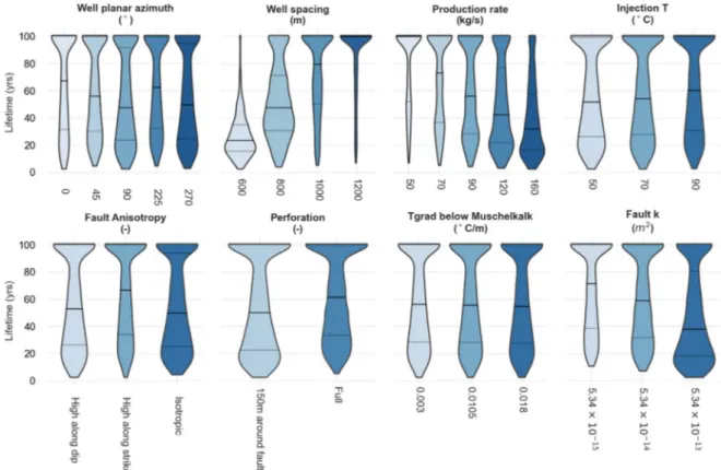
The distribution of the thermal breakthrough time (system lifetime) for all the studied cases, is shown in Fig. 3 for each

parameter and respective parameter values (de fi ned in Table 2). In this fi gure median is identi fi ed with solid horizontal line, the interquartile showed by dotted horizontal lines. The size of each line (the width of each shape) represents frequency. Comparing the median values within the variation range of each parameter it can be concluded that well spacing and production rate have the highest impact on the system lifetime. Well spacing exhibits a narrower distribution and longer lifetimes as the distance between the injector and producer well increases. Therefore, the shorter well spacing of 600 m has a very dominant effect on the system lifetime exhibiting a distribution with a median value of circa 25 years. Conversely the system lifetime is reduced with increasing production rate, while the distribution range becomes wider, expanding over more years. The highest fl ow rate of 160 kg/s ex- hibits the narrowest interquartile range with a median value of circa 33 years. High permeability along the fault dip leads to shorter lifetimes (median value of circa 54 years), while an isotropic fault permeability shifts the distribution lower with a median value of 50 years). A high permeability along the fault strike results in a dis- tribution shifted towards longer lifetimes with the highest median value of circa 55 years. The well planar azimuth (WPA) values show relatively similar distribution ranges while being different in the distribution shapes. A WPA of zero degrees shows the highest median value of circa 67 years.

The shortest interquartile range is with a WPA of 45

and 225

(35e100 years) as in these oblique angles buoyancy fl ow can expand laterally and away from the production well. The widest interquartile range is observed for 270

(median value of circa 50 years) and 90

. In both these cases the wells are oriented along the dip of the fault therefore along the gravity trace on the fault.

Buoyancy fl ow contributes to cold plume reaching the production well (WPA of 90

). This effect is countered when the producer is placed updip (WPA of 270

), slightly shifting the distribution to

Fig. 3.

Distribution of the system lifetime in years for each of the considered parameters and their values, according to eq (40) for the full dataset of 16,200 simulations. The dashed

line indicates the median value and the dotted lines the quartiles of the distribution. For simulation where the eq (40) condition is not met, the lifetime is taken equal to 100 years.

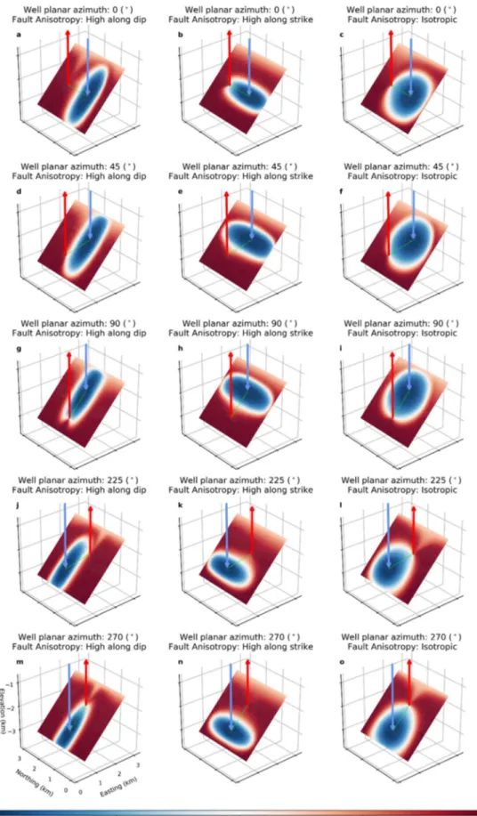
Fig. 4.

Temperature distribution on the fault plane after 30 years of production for all the combinations of well planar azimuth and fault anisotropy. The red arrow marks the

producer, the blue arrow the injector location and the lime line highlights the shortest distance between the wells on the fault plane (see results in Fig. 6). Data shown have a well

spacing of 1200 m (along the fault plane), an injection-production rate of 160 kg/s, an injection temperature of 50

C, perforation limited to 150 m above and below the fault surface,

a temperature gradient below the Muschelkalk of 30

C/km and a fault permeability of 5.34 10e13 m

.

longer lifetimes compared to a WPA of 90

.

A full perforation length increases the median value and nar- rows the distribution compared to a perforation limited to 150 m above and below the fault (medians of circa 61 years and 50 years respectively). Increasing fault permeability reduces the median and widens the distribution. This results in a system lifetime to circa 38 years for the highest permeability value of 5.34 10

m

. Injec- tion temperature has a minor effect to the overall distribution range, with a slight increase of the lower quartile and median values. Lastly, the temperature gradient below the Muschelkalk has almost no effect to the system lifetime.

3.1.2. WPA and fault permeability anisotropy

When the fault permeability is anisotropic (higher either along the dip or the strike), elongated shapes of the cold plume are observed along the direction of the high anisotropy (Fig. 4). The gravity effect becomes prominent when the producer is positioned shallower (Fig. 4m-o) and the cold plume remains deeper, covering a more restricted area due to its increased density. The opposite effect is observed when the producer well is placed updip (Fig. 4g e i) and gravity aids the colder, denser fl uid to reach the producer well. The elongated shape of the cold front is only altered when the WPA is at an oblique angle of 45

or 225

to the direction of the high permeability (Fig. 4d e f and Fig. 4j-l).

For WPA of 0

, 225

and 270

, high permeability along the fault dip leads to fast production along the dip axis (Fig. 4a, j and m respectively) as updip parts of the fault plane with lower temper- ature contribute to production. The earliest thermal breakthrough would be expected for the WPA of 90

due to gravity contributing to the movement of the cold front towards the producer. When the fault exhibits high permeability along its strike, the cold plume extends mainly along the strike axis (Fig. 4b,e,h,k,n). The cold front propagates further and it partially wraps around the producer well when the orientation of the wells is along the higher fault permeability (Fig. 4b). This suggests that this well con fi guration would encounter the earliest thermal breakthrough for a high fault permeability along the strike.

An isotropic fault permeability results in a larger fault volume accessible to the wells. As a result the cold water plume does not reach as close to the producer well when the WPA is 0

, 90

or 270

and the fault anisotropy is favourably oriented (Fig. 4b & c, g & i and

m & o). However, when the WPA is oblique (45

and 225

) the cold

plume reaches closer to the producer well under the isotropic fault permeability compared to the anisotropic cases (Fig. 4d e f and j-l).

In these oblique con fi gurations the earliest thermal breakthrough is expected for the isotropic fault permeability, despite the fact that a larger fault area is swept.

3.1.3. Cold front position and production rate

Fig. 5 demonstrates the temperature pro fi le along the shortest distance between the 2 wells for all combinations of fault anisot- ropies, well planar azimuths, and production rates. In this Fig. 0% is the injector and 100% is the producer location respectively. In all curves in Fig. 5 the cold front shape becomes sharper as the Peclet number (the ratio between convective to conductive heat fl ow) increases. Conversely, for the lower Peclet numbers (lower fl ow rate and therefore conductive dominant fl ow) the front shape be- comes more diffusive [37,64].

When the well plane is aligned to the high fault permeability the cold front covers the largest distance, resulting the earliest cold front breakthrough. This is observed for when the fault anisotropy (FA) is high along the strike and the WPA is zero degrees (Fig. 5b) and when the FA is high along the dip and the WPA is 90

and 270

Fig. 5g,m). The cold front covers the shortest distance when the WPA is perpendicular to the high fault permeability direction. This

is the case when FA is high along dip and the WPA is 0

(Fig. 5a) and when FA is high along the strike and the WPA is 90

or 270

(Fig. 5h,n). For both WPA of 90

and 270

an isotropic FA exhibits results intermediate between the favourable and unfavourable orientation of the well with respect to permeability (Fig. 5i,o). For the oblique WPA of 45

and 225

the differences between the FA orientation is minimized and the isotropic fault exhibits the larger covered distance of the cold front (Fig. 5f,l).

With an isotropic fault and a WPA of 45

the denser cold water is also assisted by gravity and exhibits an earlier thermal break- through compared to a WPA of 225

. Between a WPA of 45

and 225

the cold front distance is signi fi cantly different for the lower rates, but as the rates increase the density fl ow effect is minimized and the curves are much more similar. With the producer well positioned updip the higher rates (120 and 160 kg/s) exhibit a distinct dent in the curve around the 75% distance between the wells (Fig. 5i,o).When the WPA is oriented along the fault dip (WPA of 90

and 270

) these differences become even more apparent as the effect of gravity is maximized. All differences are less prominent as the rates are increasing as the effect of density fl ow becomes less pronounced.

The WPA of 225

and 270

that position the producer updip the temperature curve exhibits levelling off and a very sharp arrival to the production well location, which could be attributed to shal- lower parts with lower temperature contributing to the production (see also Fig. 4).

The distribution of the cold front position (see eq(43)) along the shortest distance between the wells is shown in Fig. 6. A WPA of 90

the cold front travels the longest distance between the wells, resulting in the highest median value and a distribution closer to the producer. For a WPA of 0

an almost binomial distribution is observed that can be attributed to the favourable or unfavourable WPA orientation to the fault permeability. The WPA of 45

shows an almost uniform distribution suggesting that this orientation is the least sensitive to the changes in other parameters. For both 225

and 270

WPA the shift closer to the injector is a result of the cold front having to travel against gravity towards the updip producer (see also Fig. 4). This effect is stronger for the WPA of 225

that allows the cold water plume to diverge laterally compared to the WPA of 270

where the buoyancy fl ow might be partly countered by the injector well (see also Fig. 4).

The distance covered by the cold front, after 30 years of simu- lation, decreases with the increase of well spacing. This can be attributed to two reasons: fi rstly, due to an increased well spacing increasing the reservoir volume available to the wells and secondly due to the buoyancy fl ow impact being accentuated with longer well spacing. Similarly, an increasing fl ow rate shifts the position of the cold front closer to the producer. Both these results are a complementary explanation to the system lifetime (see also Fig. 3).

With increasing injection temperature, the cold front moves closer to the injector due to a smaller temperature difference be- tween the reinjected and the reservoir fl uid and less pronounced buoyancy fl ow. This leads to small increases in the median values and slight shifting of the distribution towards the producer. The cold front propagates the least when a high fault anisotropy along the strike is present (Fig. 6); this effect can be attributed to gravity diverting larger parts of the fl ow downdip, along the preferential pathway of the permeability anisotropy (see also Fig. 4). Addi- tionally, only one considered WPA is aligned with the high fault anisotropy along the strike.

A complete perforation of reservoir thickness results in more

volume available for heat extraction and fl uid fl ow. Accordingly, a

slightly shorter interquartile distance and a slight decrease of the

cold front position is observed compared to limiting the perforation

150 m above and below the fault plane (Fig. 6). The temperature

Fig. 5.

Temperature profile after 30 years of production along the shortest distance (lime line on Fig. 4) connecting the injector well (0% distance) and the producer well (100%) for

all the combinations of rotation, fault anisotropy and injection-production rate. Data shown have a well spacing of 1200 m (along the fault plane), an injection temperature of 50

C,

perforation limited to 150 m above and below the fault surface, a temperature gradient below the Muschelkalk of 30

C/km and a fault permeability of 5.34 10

m2.

gradient below the Muschelkalk appears to have no effect on the position of the cold front with almost identical distributions. Lastly, an increasing fault permeability leads to cold front positions closer to the producer and highlights the dominant importance of permeability.

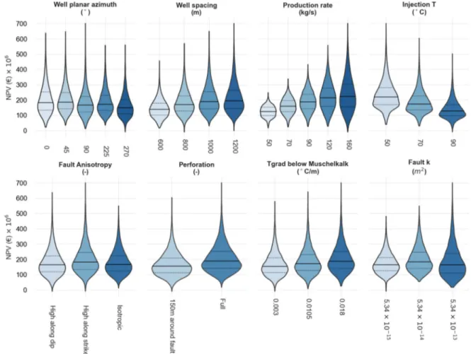
3.2. NPV and produced energy

The sensitivity of the NPV to the model inputs is showcased in Fig. 7. The WPA of 225 shows a slight reduction of the generated NPV, which is more pronounced for the WPA of 270. This decrease can be attributed to the contribution of lower temperature to the production well that is positioned updip (see also Fig. 4m-o and Fig. 5m-o). A WPA of 45

results in the highest median value and a narrower distribution towards lower NPV values. Increasing the well spacing leads to slight increases of the NPV due to extended system lifetime (see Fig. 3) resulting in higher amounts of produced energy. Increasing the well spacing improves the median NPV but also widens the distribution. Therefore, larger well spacing accen- tuates the in fl uence of other system parameters (see also Fig. 8 and Fig. 12). Similarly, higher rates also lead to wider distribution with the effective change in the distribution width being more pro- nounced that for changing well spacing. Higher rates also result in increased need for pumping that in turn decreases median NPV values if the conditions are not favourable (see also Fig. 11 and Fig. 12). Injection temperature shows a high impact as more energy can be generated from the same amount of circulated water,

resulting in high values of generated NPV with decreasing injection temperature.

3.2.1. NPV sensitivity to model inputs

The highest median NPV is observed when FA is high along the fault strike. An isotropic FA always results in lower NPV, due to earlier thermal breakthrough (see also Figs. 5 and 12) under most well con fi gurations. The narrowest distribution is encountered when the FA is high along the fault dip. Similar to injection tem- perature, increased perforation length enables more heat exchange with the layers around the fault, extending system lifetime and thus resulting in higher NPV values. The temperature gradient below the Muschelkalk also shows a positive effect to the NPV with higher gradients, but this effect is less pronounced compared to the injection temperature and the perforation length. Lastly higher fault permeability leads to lower median NPV, due to earlier ther- mal breakthrough. The distribution is also the widest suggesting that under favourable conditions higher NPV can be achieved.

The relation between system lifetime and NPV is further explored in Fig. 8. In this fi gure a more concentrated kernel sug- gests that the effect of other parameters on system lifetime and NPV is weak. Therefore, the variation of other physical and/or operational parameters do not affect the lifetime and generated NPV signi fi cantly and sensitivity and uncertainty analysis are of less value.

A well spacing of 600 m and a low production rate of 50 kg/s

results in the highest density at about 45 years and an NPV of circa

Distribution of the cold front position (X

) along the shortest streamline (lime line on Fig. 4) as a percentage of the well spacing for each of the considered parameters and

their values, according to eq. (43) for the full dataset of 16,200 simulations after 30 years of simulation. The black line indicates the median value and the dotted lines the quartiles of

the distribution.

160 M V . Gradually increasing the rates to 70 kg/s and 90 kg/s leads to shorter lifetimes and minor changes of the NPV (Fig. 8b and c).

For rates above 120 kg/s system lifetime if reduced while the NPV range widens towards higher and lower values (Fig. 8d and e). With increasing well spacing the distributions shifts towards longer lifetimes (Fig. 8f,k,p), while the generated NPV range does not change. With a well spacing of 1200 m no thermal breakthrough (as described in eq (40)) for rates of 50 kg/s or 70 kg/s respectively (Fig. 8p,q).

Considering a rate of 160 kg/s and a well spacing 800m, we observe a strong kernel (Fig. 8j). The largest well spacing and higher rates (1200 m and 160 kg/s respectively, Fig 8t) results in the widest spread in the distribution of both the NPV and the system lifetime and the kernel is not as concentrated. The distribution results in NPV close to zero under some cases, despite the long system life- times (see also Fig. 12). This shows that the variation of other pa- rameters impact both the lifetime and NPV signi fi cantly. In this scenario, sensitivity and uncertainty analysis over the parameters has utmost importance and its further explored in Fig. 12.

3.2.2. NPV and system lifetime

Changes in the distribution of the generated NPV for the subset of 1200 m well spacing and the high rates of 160 kg/s are further explored in Fig. 9. With regards to the injection temperature the largest changes are observed when the wells are oriented along the strike (WPA of 0

) or when the producer is positioned updip (WPA of 225 and 270). In these cases, the shape of the distribution changes and becomes less wide when the injection temperature is

increased. Increasing the injection temperature has the least negative effect when the producer is positioned downdip (WPA of 45

and 90

). In this case increasing the injection temperature does not alter the distribution shape.

Fault permeability values have the strongest impact when the producer is positioned downdip (WPA of 45

and 90

). For the WPA of 45

and 90

the reduction in fault permeability (regardless of any anisotropy) is enough to alter the NPV distribution from a very wide distribution to a very narrow one as fault permeability is reduced;

Therefore, when the producer is downdip the low fault perme- ability becomes dominating for the NPV.A WPA along the fault strike is the least affected by the permeability of the fault both in terms of mean values but also in distribution shape, meaning that it is the most robust choice under uncertainty of the fault permeability.

A longer perforation length always results in increased gener- ated NPV as it prolongs the production of higher temperatures due to increased heat exchanged with the surroundings formations. The effect is comparable for all WPA without signi fi cant changes in the distribution shape between the different perforations.

An increased temperature gradient for the layers below the Muschelkalk also improved the NPV for all considered WPA. The most prominent impact gain is when the WPA are either along the fault strike (WPA of 0

) or the producer is positioned downdip (WPA of 45

and 90

). The reason is that downdip wells are also encountering deeper layers that are more affected by the increased gradient.

Fig. 7.

Distribution of the generated NPV for each of the considered parameters and their values, for the full dataset of 16,200 simulations at the time of thermal breakthrough. The

black line indicates the median value and the dotted lines the quartiles of the distribution.

3.2.3. NPV and WPA

Parameters that improve the ef fi ciency of heat extraction do have a more prominent effect on the produced energy (Fig. 10).

Increasing the injection temperature greatly impacts the cumula- tive energy produced; the impact is negative and more pronounced between 70

C and 90

C compared to 50

C and 70

C. Similarly, the impact of the temperature gradient below the Muschelkalk is mi- nor but leads to a longer distribution tail towards higher energy production.

Increasing the well spacing and the rate shifts the distribution to larger amounts of generated energy. Nonetheless rates above 70 kg/

s showcase very similar median values but with increasingly higher upper quartiles. For the WPA an orientation along the fault strike (WPA of 0

) has the widest distribution, suggesting that in the presence of uncertainties it is the optimal orientation for ensuring larger amounts of produced energy (see also Fig. 9).

Isotropic fault permeability results in the lowest distribution, with high anisotropy along the strike resulting in the higher me- dian and quartile values. Low fault permeability leads to larger amounts of produced energy through the prolonging of the thermal breakthrough. However as seen earlier (Fig. 9) this does not result in higher NPV.

3.2.4. NPV and produced cumulative energy

The relation between the produced amount of energy and the generated NPV is depicted in Fig. 11. While higher rates do result in larger amounts of produced energy this is not directly correlated to the NPV. The required pumping energy is the controlling factor between negative and positive NPV. For rates up to 90 kg/s we see a strong clustering of the data and a linear increase of the NPV with the cumulative produced energy. From 120 kg/s onward the spread in the data increases. Notably, the WPA with the producer wells either along the strike (WPA 0

) or downdip (WPA of 45

and 90

) show a stronger correlation between increased generated energy and increased NPV (Fig. 11e,j,o). For the other WPA orientations the linear increase of NPV with the cumulative produced energy is only maintained with the fault is isotropic (Fig. 11t,y).

3.2.5. Economic ef fi ciency

The ratio between the generated NPV and the cumulative en-

ergy produced is analysed in Fig. 12. For well spacing of 600 m

increasing the rates always results in an increased ratio. This in-

crease is minimal when the WPA is oriented along the high value of

the fault anisotropy (Fig. 12b,g,m). In this case the NPV per pro-

duced MWh is already high with low rates and increases only

Kernel density estimation of system lifetime (xaxis) with the generated NPV (yaxis) for the combinations of Rates (columns) and well spacing (rows) for the full dataset of

16,200 simulations. Kernel density estimation is performed per subplot and is therefore not comparable between subplots. In each plot yellow shows high and blue low density.

slightly with higher rates. With the same well spacing and reducing fault permeability to 5.34 10

m

the NPV per produced MWh increases when the rates increases up to 90 kg/s. Beyond 90 kg/s diminishing returns are encountered: slight increases when the WPA is favourably oriented with respect to the fault anisotropy (Fig. 12g) and reduction of the value per MWh produced when the orientation is unfavourable (Fig. 12b). Further reducing the fault permeability ampli fi es this impact, therefore, 90 kg/s emerges as an optimum production rate if fault permeability is not the highest.

With a well spacing of 1200 m the NPV per produced MWh exhibits a strong increase with increasing fl ow rates when the fault permeability is highest and the fault permeability is isotropic.

Similarly to the 600 m well spacing, this effect is minimized when the WPA is oriented favourably with respect to anisotropy (Fig. 12b,g,m). Increasing the rates seems to improve the NPV per MWh more when the producer is positioned updip (Fig. 12m). A fault permeability of 5.34 10

only shows a slight increase of value per MWh under all WPA when the fault permeability is isotropic. For anisotropic fault permeability when the orientation of the WPA is favourable the value per MWh increases with increasing rate, but shows no improvement when increasing the rate from 120 kg/s to 160 kg/s (Fig. 12b,g,m). Lastly, the NPV per MWh for the low fault permeability and the 1200 m well spacing only reduces with increasing rates.

4. Discussion

The results of this study show that - depending on the selected criteria - gauging the general performance of the geothermal res- ervoirs (lifetime, energy and NPV) results in different (sometimes opposing) outcomes. As shown in Fig. 3, an increase in fault permeability signi fi cantly reduces the lifetime of the reservoir

whereas the NPV analysis of the same inputs (Fig. 7) represents a notable increase for higher fault permeability values at favourable operational conditions. This can be explained due to the unfav- ourable connection between the two wells at higher fault perme- ability that shortens the system's lifetime whereas the decrease in the required pumping power may lead to more generated NPV.

Additionally, the pumping requirements are not high enough to result in NPV reduction, despite the increased pumping pressure needed for the lower permeability (see also Fig. 11).

It is observed that uncertainty in the thermal gradient inside reservoir section has a minor in fl uence on the reservoir lifetime (see Fig. 3) in contrast to its in fl uence on the NPV of the reservoir (see Fig. 7) which is more signi fi cant. This effect can be attributed to the importance of the buoyancy effect on the reservoir perfor- mance. It is however, noteworthy to mention that larger thermal gradients would be a manifestation of the lower permeability which would impede the natural hydrothermal convection in the system, which can also be linked to the lower NPV in such reservoirs.

The analysis of the Kernel density in Fig. 8 shows that the in-

crease in the injection fl ow rate for a well spacing of 600 m will

reduce the uncertainty associated with the predicted system life-

time. Contrary to this, a longer well distance for a given fl ow rate

results in a broader range in predicted reservoir lifetime (Fig. 8). In

the presence of uncertainty with regards to fault permeability and

anisotropy, oblique angles prove more resilient for thermal break-

through compared to directions aligned with the high anisotropy

axis (Figs. 5 and 6). This can be a result of the interaction between

the higher sweep ef fi ciency with the main fl ow direction aligned

with the lower permeability axis compared to the lower pressure

impedance along the higher permeability direction of the anisot-

ropy. Favourable orientation with regards to the anisotropy axis can

Distribution of the NPV for each well planar azimuth and the extreme values of injection temperature, fault permeability, perforation and temperature gradient below

Muschelkalk for the subset of data with a well spacing of 1200 m and an injection-production rate of 160 kg/s. The black line indicates the median value and the dotted lines the

quartiles of the distribution.

be bene fi cial with regards to NPV (Fig. 7), although it might result in lower system lifetime (Fig. 3). Therefore, initial geological in- dications of possible fault permeability anisotropy direction can be of critical importance in designing the well con fi guration. Similar importance to subsurface parameters for techno-economic de- cisions have been highlighted for EGS projects [65]. Additionally, placement of the production well updip is associated with reduced NPV of the system due to the lower production temperature encountered at shallower depths (Figs. 7 and 9).

Identifying and characterizing the presence of fault anisotropy is crucial for the optimal orientation of the wells with regards to the high permeability anisotropy axis. High fault permeability, regardless of possible anisotropy on the fault, is associated with a signi fi cant increase in NPV (Figs. 7 and 9), the uncertainty of which can be further reduced by selecting a proper well placement strategy in terms of orientation (Fig. 9) and spacing (Fig. 8). If characterisation is not possible, results presented herein show that an oblique angle (e.g. WPA of 45

and 225

) is the most robust well con fi guration strategy to improve the prediction and reduce the uncertainty of NPV, system lifetime and economic ef fi ciency (Fig. 9).

The NPV of the system increases with an increase in production fl ow rate which is consistent with previous NPV studies of geothermal systems [7,10,17,65]. However, the associated NPV range signi fi cantly grows at higher fl ow rate (see Fig. 8) and higher fl ow rates can also reduce the economic ef fi ciency when perme- ability is lower. While higher rates do result in larger amounts of produced energy this is not directly correlated to the NPV (Figs. 8

and 12), as it was previously modelled in faulted hydrothermal systems with formation intervals acting as the main reservoir and fl uid pathway [7,66]. Therefore, for systems with the fault plane as the main fl uid pathway and in the presence of uncertainty, decreasing the well spacing can lead to a reduced range in the generated NPV, hence increasing decision making con fi dence (Fig. 12). For shorter well spacing however, it is more important to characterize fault anisotropy compared to when a large well spacing (Fig. 12) is used.

Under the considered uncertainty ranges, there exists an opti- mum fl ow rate and well spacing beyond which the economic ef fi - ciency of the system can be signi fi cantly reduced (Fig. 12).

Production rates above 90 kg/s show diminishing returns with regards to the generated NPV in most cases (Fig. 12). Larger well spacing reduces the economic ef fi ciency of the system which de- creases with increasing rate for the low permeability cases regardless of well orientation (Fig. 12). Signi fi cant improvements in economic ef fi ciency with increasing the production rate above 90 kg/s are only achieved when the wells are oriented favourably with the anisotropy axis that exhibits higher permeability. This improvement prevails also for larger well spacing.

The buoyancy effect is signi fi cant at lower fl ow rates at which

the forced convection effects become less dominant. With the

highest rates used in our study (160 kg/s) the differences between

positioning the producer updip (WPA of 270

) compared to

downdip (WPA of 90

) are negligible (Fig. 5). However, these dif-

ferences are signi fi cant for rates up to 90 kg/s and favour the

placement of the producer downdip as this combines the effect of

Distribution of the produced cumulative energy for each of the sensitivity parameters, for the full dataset of 16,200 simulations. The dashed line indicates the median value

and the dotted lines the quartiles of the distribution.

higher production temperatures due to the geothermal gradient (Figs. 5 and 11). The modelling of the cold front position can inform on how we can better manage the resource when using the fault as the main fl uid pathway (Fig. 5). In the case of placing the producer updip, the differences in the cold front position between high and low rates (Fig. 5) aid in identifying the presence and signi fi cance of density driven fl ow in retarding the cold front from reaching the producer well. The results are consistent with the study carried out by Bataill e et al. (2006). While the economic ef fi ciency is reduced, placing the injector well downdip could help with retaining the cold-water plume deeper when low rates are used, therefore pro- longing system lifetime (Figs. 4 and 5). In this case, the cooled down plume might exhibit a much larger extent with implications to pressure dissipation and possible fault stability (Fig. 4).

Full factorial design studies such as the one presented here further our understanding of system dynamics under uncertainty, despite the ef fi cient computation design (see section Reservoir

model) remain computationally expensive due to the large number of simulations required (16,200 simulations in this study). Recent advances in reservoir simulation open new possibilities in terms of comprehensive evaluation of uncertainties. The newly presented DARTS simulator is highly ef fi cient [67] in CPU based simulation and is also developed to run on GPU, improving the computation time by 8e10 times [68]. These developments open-up new pos- sibilities for both extensive studies on uncertainty in heteroge- neous, fl uvial geothermal systems [22] but also for further computational ef fi ciency in optimisation studies [10].

Uncertainty related in the temperature gradient below a certain depth have minor effects on the lifetime but can impact the NPV since they directly affect the produced temperature. Previous studies have highlighted the importance of thermal anomalies [69]

and high thermal conductivity of lithostratigraphic layers [70] to

the power output of geothermal systems. Our analysis shows that

the uncertainty related to the geothermal gradient in this study has

Cumulative produced energy (MWh) against generated NPV for the combinations of injection and production rates and well planar azimuth. Data is coloured by the

required pumping energy and coded according to the fault anisotropy. The dataset is limited to a well spacing of 1200 m.

almost no effects on the system lifetime and minor effects in the amounts of generated energy and NPV. This can be attributed to the relatively low permeability of the formations and against the much larger permeability of the fault as the main fl uid pathway in our

study. The larger permeability of the fault compared with the for-

mation, also imply that the potential hydrothermal convections

inside the fault over geological timeframe as well as during the

project's lifetime (due to forced circulation) can signi fi cantly reduce

NPV per cumulative energy produced (V/MWh) against the different

permeability (colour) and well spacing (line/symbol). The dataset shown here uses a perforation limited to 150m above and below the fault, an injection temperature of 50

C and a

temperature gradient below the Muschelkalk of 0.003

C/m.