Using acoustic metrics to characterize underwater acoustic biodiversity in the Southern Ocean

(1)

Using acoustic metrics to characterize underwater acoustic biodiversity in the Southern Ocean

Irene T. Roca¹ & Ilse Van Opzeeland^1,2

1Helmholtz Institute for Functional Marine Biodiversity at the University of Oldenburg (HIFMB), Ammerl€ander Heerstraße 231, 26129, Oldenburg, Germany

2Ocean Acoustics Lab, Alfred-Wegener Institute (AWI), Helmholtz Centre for Polar and Marine Research, Klussmannstrasse 3, 27570, Bremerhaven, Germany

Keywords

Acoustic metrics, Antarctic, community composition, marine acoustic environments, passive acoustic monitoring, species diversity Correspondence

Irene T. Roca, Helmholtz Institute for Functional Marine Biodiversity at the University of Oldenburg (HIFMB), Ammerl€ander Heerstraße 231, 26129, Oldenburg, Germany. Tel: +49 (471) 4831 2568; Fax: +49 (471) 4831 1149; E-mail:

iroca@hifmb.de Editor: Nathalie Pettorelli Associate Editor: Nicola Quick

Received: 28 June 2019; Revised: 26 August 2019; Accepted: 3 September 2019

doi: 10.1002/rse2.129

Abstract

Acoustic metrics (AM) assist our interpretation of acoustic environments by aggregating a complex signal into a unique number. Numerous AM have been developed for terrestrial ecosystems, with applications ranging from rapid biodiversity assessments to characterizing habitat quality. However, there has been comparatively little research aimed at understanding how these metrics perform to characterize the acoustic features of marine habitats and their relation with ecosystem biodiversity. Our objectives were to 1) assess whether AM are able to capture the spectral and temporal differences between two distinct Antarctic marine acoustic environment types (i.e., pelagic vs. on-shelf), 2) evaluate the performance of a combination of AM compared to the signal full frequency spectrum to characterize marine mammals acoustic assemblages (i.e., species richness–SR–and species identity) and 3) estimate the contribution of SR to the local marine acoustic heterogeneity measured by single AM. We used 23 different AM to develop a supervised machine learning approach to discriminate between acoustic environments. AM performance was similar to the full spectrum, achieving correct classifications for SR levels of 58% and 92% for pelagic and on-shelf sites respectively and>88% for species identities. Our analyses show that a combination of AM is a promising approach to characterize marine acoustic communities. It allows an intuitive ecological interpretation of passive acoustic data, which in the light of ongoing environmental changes, supports the holistic approach needed to detect and understand trends in species diversity, acoustic communities and underwater habitat quality.

Introduction

Contrary to what was thought during much of the 20th century, underwater marine environments are filled with sounds. Many aquatic organisms produce and rely on acoustic cues as primary source of information about their environment (e.g. Montgomery et al. 2006; Simpson et al. 2011; Fais et al. 2016). In the oceans in general and in polar regions in particular, access to visual species distribution and abundance is often limited, making biodiversity monitoring challenging or even impossible in particular seasons. Passive acoustics has emerged as an attractive alternative to conventional sampling techniques to collect data, monitor acoustic biodiversity and evaluate

the effects of the acoustic structure of the landscape on the abundance and distribution of terrestrial and aquatic organisms (Van Parijs et al. 2009; Pijanowski et al. 2011).

In marine and polar habitats, the versatility of passive acoustic recordings to remotely assess acoustic behaviour and biodiversity was realized over 50 years ago (Watkins 1963; Watkins and Schevill 1968). Consequently, passive acoustic datasets from particular regions currently consti- tute extensive and ecologically valuable databases (e.g.

Nishimura and Conlon 1994; Boebel et al. 2006 and Van Parijs et al. 2009 for a review). Nevertheless, the analysis of these large passive acoustic datasets continues to be a hurdle. Visual and aural processing of long-term, large scale passive acoustic recordings by analysts is often

(2)

infeasible in real-time. Automated call detectors provide faster routines, yet they need to be calibrated for every species and acoustic context and revised for missed calls and false detections, which is also time consuming (e.g.

Baumgartner and Mussoline 2011; Leroy et al. 2018).

Over the last decade, several metrics have been pro- posed to describe the variety of acoustic structures pro- duced by both biotic and abiotic sound sources (e.g.

Sueur et al. 2014). Acoustic metrics (AM) assist our interpretation of acoustic environments by aggregating the acoustic information of a complex signal into a unique number. They provide a rapid and intuitive solution to analyse large passive acoustic data and can be generalized to be applied to very different datasets. So far, AM have been successfully used for different purposes in terrestrial ecosystems and tested in some aquatic ones, including: as proxies to perform rapid biodiversity assessments (e.g.

Sueur et al. 2008b; Pieretti et al. 2011; Depraetere et al.

2012), to model community assemblage patterns (Roca and Proulx 2016), to describe spatial heterogeneity and habitat type (e.g. Tonolla et al. 2011; Bormpoudakis et al.

2013; McWilliam and Hawkins 2013; Lillis et al. 2014), to quantify anthropogenic noise pollution (Buxton et al.

2017), to evaluate the effect of human-induced noise on animal behaviour (e.g. Joo et al. 2011; Kasten et al. 2012) and to assess habitat quality or ecological condition (e.g.

Gordon et al. 2018). However, to date, there has been comparatively little research aimed at using AM to understand the variations in acoustic features of marine habitats and their relation with the ecosystem biodiversity structure and dynamics.

According to the acoustic niche hypothesis, the acoustic environment can be represented as a resource that is shared by vocalizing animals (Krause 1987). Co-occurrent species produce species-specific spectral and temporal communication patterns (L€uddecke et al. 2000; Sueur 2002) that may have evolved to minimize acoustic inter- ference among one another. A consequence of this spe- cialization is that the acoustic heterogeneity of a community is predicted to increase with the number of vocalizing species within it. Several studies have found evidence of such acoustic partitioning to occur in different terrestrial and aquatic acoustic communities (e.g.

Planque and Slabbekoorn 2008; Schmidt et al. 2013;

Ruppe et al. 2015) and some of them have successfully used specific AM to quantify the acoustic heterogeneity- species diversity relationship (e.g. Sueur et al. 2008b; Pier- etti et al. 2011; Villanueva-Rivera et al. 2011; Depraetere et al. 2012). However, these positive relationships and the possibility to use AM as a standard and rapid tool (e.g. as proxies) to perform rapid biodiversity assessments have so far yielded mixed results in marine ecosystems. Some studies showed that particular metrics did adequately

mimic biotic acoustic activity and species diversity (Parks et al. 2014; Bertucci et al. 2016; Harris et al. 2016; Pieretti et al. 2017), while others considered indices suboptimal to track marine acoustic diversity (Bohnenstiehl et al.

2018; Buxton et al. 2018; Lyon et al. 2019). Most of these earlier studies evaluated the potential to use single AM in shallow fish and shrimp-dominated underwater environments to estimate diversity which was characterized by biodiversity proxies (recognizable acoustic units) or visual biodiversity records. The only study assessing the potential of AM to estimate marine mammal diversity in deep oceanic waters evaluated the performance of one single acoustic index, i.e., the acoustic entropy index H (Parks et al. 2014), to predict biotic acoustic activity. Parks et al.

(2014) found a positive relationship between a noise- compensated H index (HN) and the number of whale calls per hour.

Here we apply a suite of AM, including some acoustic heterogeneity metrics, to characterize the marine mammal community composition using a large passive acoustic dataset from an area with relatively low anthropogenic noise. We intentionally used the raw passive acoustic recordings (i.e., without previous signal filtering) spanning 10 years and five sites to evaluate the general and practical applicability of such rapid acoustic diversity assessments. Our objectives were: (1) to assess whether AM are able to capture the spectral and temporal differences between two distinct acoustic environment types (i.e., pelagic vs. on-shelf) in our database, (2) to evaluate the performance of a combination of AM compared to the signal full frequency spectrum to discriminate between the acoustic species richness levels and the identities of the species comprising the marine mammal communities, and (3) to estimate the contribution of species richness to the local marine acoustic heterogeneity measured by single AM.

Material and Methods

Study sites and acoustic recordings

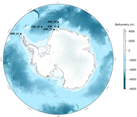
Data were obtained from five recording sites situated in the Atlantic section of the Southern Ocean (Weddell Sea basin; Fig. 1) over 10 years (2008–2017). The Southern Ocean represents one of the last relatively pristine marine acoustic environments on Earth (Halpern et al. 2015;

Jones et al. 2018), mainly composed of biotic sounds coming from marine mammals and abiotic sounds from storms, sea-ice and glacier calving (Menze et al. 2017).

Recordings were part of the big database collected since 2006 by the acoustic recording network in the Weddell Sea (Boebel et al. 2006; Rettig et al. 2013). We used AURAL- M2 recordings (Autonomous Underwater Recorder for

(3)

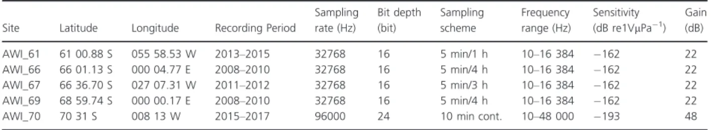
Acoustic Listening-Model 2, Multi-Electronique Inc 2016) from four pelagic sites (AWI_61, AWI_66, AWI_67 and AWI_69; Table 1). We define pelagic here as>30 km from the Antarctic ice shelf and>300 m of seafloor depth. We selected recording sites based on their geo- graphic location covering potentially different oceanic acoustic environments and marine mammal communities across the Weddell Sea area. Recorders were attached to oceanographic deep-sea moorings of the Hybrid Antarctic Float Observation System (HAFOS, Rettig et al. 2013). The acoustic recorders were moored at ~ 200 m depth and set to different duty cycles (see Table 1) due to constraints of battery life and data stor- age capacities. All AURAL recorders were equipped with HTI-68-MIN hydrophones (High Tech Inc., Long Beach, USA; please refer to Menze et al. (2017) and Table 1 for further technical details on the recordings). The fifth recording site (AWI_70; Table 1) was situated on the edge of the Eckstr€om Ice shelf (also known as PALAOA, see Boebel et al. 2006, but hereinafter referred to as the on-shelf site). Recordings were made using a Sono.Vault recorder (Develogic GmbH, Hamburg, Germany) con- nected to an active RESON TC4032 hydrophone suspended in the water column 70 m beneath the ice shelf (~160 m thick) and at 90 m above the seafloor (see Boebel et al. 2006 and Table 1 for further details on the recordings).

Acoustic analysis

We performed a stratified random sampling over the available temporal acoustic data per site (see 1) to select acoustic recordings to include in the analysis. For each site, we searched for an even repartition into species richness levels (SR) and a balanced representation of naturally occurring species in the different community composi- tions. A dataset comprising 921 acoustic environments over the five sites and 10 years was selected for analysis.

All acoustic recordings used for further analysis were clipped to 5 min length and decimated to 5000 Hz sampling frequency to obtain a better resolution for the calls of the most frequent marine mammal species detected in the Weddell Sea (Boebel et al. 2009). Clipping and deci- mating of data was performed in MATLAB R2017b. We manually assessed acoustic presence/absence of the different marine mammal species for every 5 min recording through a visual and aural inspection of the data using spectrograms in Raven Pro 1.5 (Cornell Lab of Ornithol- ogy, Ithaca, NY, USA). Spectrogram settings for this task were adapted to optimize the display of the different species call patterns to facilitate identification. The SR level of each recording was determined by the number of species that co-occurred in the 5 min sound file.

We used the function meanspec from theseewavepack- age (Sueur et al. 2008a) in R (version 3.5.2; R Core Team

Figure 1. Map of the five mooring locations in the Southern Ocean.

(4)

2018) to extract the full frequency spectrum (hereinafter referred to as full spectrum) of every 5 min acoustic file (short-term Fourier transform with a 50% window overlap and 512 window length) yielding 256 amplitude values for the 0-2500 Hz frequency range per acoustic file.

In addition, we computed 23 different AM (see detailed list in Table S1) for every acoustic file. Among these 23 AM we included those that have been shown to exhibit good performance in different contexts when undertaking rapid biodiversity surveys in terrestrial environments, some of which have also been used to assess acoustic biodiversity for aquatic ecosystems. The metrics we used can be classified in three categories: (1) indices based on different algorithms to compute acoustic complexity, entropy or heterogeneity (a indices); (2) metrics measur- ing amplitude or background patterns; and (3) metrics computing ratios between acoustic activity in different frequency bands. To compute the selected AM, we used several functions fromtuneR (Ligges et al. 2016), seewave and soundecology(Villanueva-Rivera and Pijanowski 2018) packages in R.

Statistical analysis

To evaluate the potential of AM to capture the difference in spectral and temporal patterns between on-shelf and pelagic sites, we used the K-means clustering algorithm.

K-means (MacQueen 1967) is an unsupervised machine learning algorithm that iteratively partitions a given dataset into a set of k clusters (i.e., k groups; where k represents the number of clusters) aiming to minimize the total intra-cluster variation (i.e., high intra-class similarity and low inter-class similarity). Intra-cluster variation is computed as the sum of squared Euclidean distances between points and the corresponding centroid. In this study we applied the cascadeKM function within the vegan package (Oksanen et al. 2018) in R to compute several k-mean partitions forming a cascade from small to large k values. We tested from 2 to 5 clusters (since we only had five different sites) and used the ‘Simple Struc- ture Index’ (ssi; Dolnicar et al. 1999) to determine the correct number of groups. Ssi varies between 0 and 1,

where maximum values indicate the best number of clusters. It is computed by normalizing the product of three elements: the maximum difference of each variable (i.e.

AM) between the clusters, the sizes of the most contrast- ing clusters and the deviation of a variable in the cluster centres compared to its overall mean. We used a principal component analysis biplot (PCA biplot) to visualize the variation in the acoustic patterns (characterized by the linear combination of 23 AM) among the 921 acoustic environments and the cluster analysis results.

We used the Boruta algorithm (Kursa and Rudnicki 2010) to select relevant variables (for AM and full spectrum respectively) to include in random forest classification models. The Boruta algorithm iteratively removes the variables that are statistically less relevant than random probes. A random probe is a ‘shadow’ variable, whose values are obtained by shuffling values of the original variable across objects. The algorithm then, performs a classification using all attributes (original variables and random probes) and computes their importance. The importance of a shadow attribute can be nonzero only due to random fluctuations. The set of importance of shadow attributes is used as a reference to decide which original variables are truly important. We used the Boruta function from the Boruta package (Kursa and Rudnicki 2010) in R.

To test the ability of AM and the full spectrum to discriminate between SR levels we developed separate random forest models (Breiman 2001). We developed two models for each site type (i.e., pelagic and on-shelf), one model included AM whereas the other included full spectrum as input variables, resulting in a total of 4 models.

To assess AM accuracy to discriminate between species identities we developed a random forest model per species. We used the randomForest function in R ran- domForest package (Liaw and Wiener 2002) and for each model we grew 1001 trees and tested sqrt(p) predictor variables at each split (where p is either the number of AM or frequency bands). For each tree constructed in a random forest, 2/3 of the data are subsampled to train the classification model and 1/3 of the data are left out to test the model (i.e., Out-of-bag or OOB cases). The

Table 1. Technical information on recorders per site. Recorders used coordinated universal time

Site Latitude Longitude Recording Period

Sampling rate (Hz)

Bit depth (bit)

Sampling scheme

Frequency range (Hz)

Sensitivity (dB re1VlPa ¹)

Gain (dB)

AWI_61 61 00.88 S 055 58.53 W 2013–2015 32768 16 5 min/1 h 10–16 384 162 22

AWI_66 66 01.13 S 000 04.77 E 2008–2010 32768 16 5 min/4 h 10–16 384 162 22

AWI_67 66 36.70 S 027 07.31 W 2011–2012 32768 16 5 min/3 h 10–16 384 162 22

AWI_69 68 59.74 S 000 00.17 E 2008–2010 32768 16 5 min/4 h 10–16 384 162 22

AWI_70 70 31 S 008 13 W 2015–2017 96000 24 10 min cont. 10–48 000 193 48

(5)

general misclassification rate of the model (general OOB estimate) is computed as the average across all OOB cases and trees. We used the Gini index as a measure of the reduction in misclassification error (i.e., variable importance) when including an additional predictor variable (either AM or a frequency band) in the model. We additionally developed a random forest model using the 23 AM to determine the most important variables discriminating between the obtained clusters.

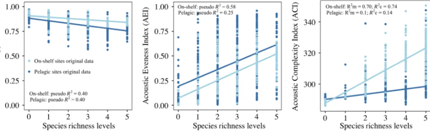
To test the effect of the community composition on the local acoustic heterogeneity of both on-shelf and pelagic sites, we fitted a regression model for each of three single acoustic heterogeneity metrics [acoustic entropy index (H), acoustic evenness index (AEI) and acoustic complexity index (ACI)], for pelagic and on-shelf sites separately. We fitted beta regression models (Ferrari and Cribari-Neto 2004) for H and AEI to account for the fact that both indices are mathematically bounded between 0 and 1. We used the betareg function from the betareg package in R (Cribari-Neto and Zeileis 2010) and included SR and year as fixed predictor variables. For ACI we fitted linear mixed-effects models using the lmer function from thelme4package in R. We included SR as fixed effect and year as random effect variable. Year was included to account for the unbalanced temporal variability of the acoustic heterogeneity at pelagic and on-shelf sites. To evaluate the goodness-of-fit of the models we used pseudo R²for the beta regressions and marginal and conditional coefficient of determination for the linear mixed-effect models.

Results

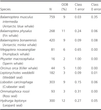
Acoustic assemblages in our study area were mainly comprised by 0 to 5 co-occurring species from an observed regional pool of 10 different marine mammal species (Fig. 2). We registered the acoustic presence of four Balaenopteridae species, one Physeteridae, one Del- phinidae and four Phocidae species (Tables 4 and S2). No other biophonic sounds (e.g. fish or invertebrates) were detected. Very few recordings (0.3%) showed more than five species vocalizations co-occurring in the same 5 min files and they occurred only in one of the five sites (AWI_61).

Cluster analysis results showed that the best partition achieved by the AM for the acoustic environments in our study area and according to the ssi criteria was two (k =2; Fig. 3). The first cluster, hereafter referred as

‘pelagic cluster’, comprised 70%, 80% and 78% of AWI_66, AWI_67 and AWI_69 acoustic environments respectively. The second cluster, henceforth called ‘on- shelf cluster’, comprised 90% of AWI_70 acoustic environments and 60% of AWI_61. Random forest

classification showed that AM achieved a highly accurate discrimination between pelagic and on-shelf clusters (OOB=2.28%). Variable importance showed that the pelagic cluster was characterized by high background to biotic signal ratios and low acoustic heterogeneity. Acous- tic environments included in the on-shelf cluster had higher sound pressure levels, lower background to biotic ratios and higher acoustic heterogeneity (Fig. 3).

Random forest results showed that full spectrum and AM achieved very similar accuracy in the classification of SR and species identity. For pelagic sites, full spectrum signatures, after Boruta variable selection, performed slightly better than the AM (OOBspec=38% vs. OOBac.- metrics=42%; 2). For the on-shelf site, classification per- formances were similar between full spectrum signatures and AM (OOBspec=9.7% vs. OOBac.metrics=9.8%;

Table 3). For both the on-shelf and pelagic models, the AM that better discriminated between SR levels were background level, mean spectral power level and ACI, yet, the Boruta algorithm considered all 23 metrics relevant for the classification. The performance of the AM differed slightly from that of the full spectrum to classify species identities, being it higher or lower according to the species (Tables 4 and S3). In general, the misclassification error of the model using AM was lower than 15%.

The acoustic heterogeneity variation represented by H, AEI and ACI metrics was better explained by SR levels in on-shelf than in pelagic sites. Pseudo and marginal R² values were>40% for on-shelf and <40% for pelagic sites (see Fig. 4). AEI and ACI showed a positive relationship with SR while H showed a negative one. Both SR and year had significant effects on acoustic heterogeneity variation (Table S4).

Discussion

This study provides the first positive results in applying a combination of AM to discriminate between acoustic assemblage composition in marine acoustic environments.

We obtained highly accurate classification models for SR in on-shelf sites (Table 3) and for species identity in general (Table 4). The model using AM to discriminate between SR levels in pelagic sites performed with an accuracy higher than 50% and was comparable to the model using the full spectrum. However, the high prevalence of background noise over the biotic signals in these acoustic environments prevented higher classification accuracy. We additionally show that in general, variation in acoustic heterogeneity was better explained by SR in on-shelf sites compared to pelagic ones, suggesting a potential to use single acoustic heterogeneity metrics for rapid biodiversity surveys in marine environments similar to the ones recorded in on-shelf sites.

(6)

Figure 2. Spectrograms showing two examples of low A. and high B. diverse acoustic environments from the Weddell Sea. Spectrograms were computed using a Fourier window size of 1024 samples and an overlap of 50%.

Figure 3. Cluster analysis results based on k-means algorithm. Cluster analysis was applied to the matrix containing 23 AM computed for each of the 921 acoustic environments. PCA biplot shows the variation in the acoustic patterns (characterized by the linear combination of 23 AM) among these 921 acoustic environments along the first two principal components. Point colour illustrates the cluster to which each acoustic environment belongs according to the k-means algorithm and the ssi criteria (on-shelf or pelagic). Ellipses represent the 95% quantile ellipse of the two identified clusters. We additionally draw the AM that better discriminated between acoustic environments to classify them into the two observed clusters (OOB = 2.28%). BP, SPL, BL, H and ACI represent background noise level percentile, mean sound pressure level, background noise level, Acoustic entropy index and Acoustic complexity index respectively (see Table S1 in Supp. Mat. for further description).

(7)

Acoustic environments in the Weddell Sea We hypothesized that the variation in acoustic spectral and temporal patterns between on-shelf and pelagic acoustic environments was higher than within pelagic sites. Recordings at the pelagic sites (AWI_61, 66, 67, 69) were made with moored devices at water depths between 300 and 5000 m depth with strong seasonal fluctuations in local ice cover. The on-shelf site (AWI-71) hydrophone was suspended in the water column less than 300 m deep and was permanently shielded by the overhanging ice shelf. The specific conditions of the location of this on- shelf site provide a very particular acoustic environment characterized by the intensity and clarity of particular marine mammals calls, such as the four most abundant Antarctic seal species (Table S2). Furthermore, pelagic sites may be more likely to have transiting animals, whereas shelf areas may be zones where animals are more prone to stay longer, either because of the coastal polynya granting them access to open water when needed, or the local upwelling providing them foraging opportunities.

This is congruent with our result, showing that on-shelf acoustic environments are characterized by higher sound pressure levels, lower background to biotic signal ratios and higher acoustic heterogeneity. The cluster analysis revealed two distinct clusters that mainly represented the acoustic environments from on-shelf and pelagic sites respectively. The association of most sites to one or other cluster was clear and could be explained by their physical position in the Weddell Sea basin and their acoustic environment patterns. However, this was not the case for site AWI_61, which was considered a pelagic site, but showed a 60% association to the on-shelf cluster. This could be partially explained by the acoustic properties of the 0 and 1 SR level acoustic environments from AWI_61 site, which were similar to the AWI_71 ones, in that the sum of energy from 200 to 2500 Hz frequency band was higher than in other acoustic environments. While in AWI_71 this pattern was due to the occasional presence of vessel noise, it is impossible to know the source in AWI_61 case because it is integrated in the background noise and visually or aurally unidentifiable.

AM to characterize marine acoustic community composition

The advantage of using the full spectrum in a classification model lies in that it conserves the complete acoustic information present in the audio files. However, classification models fitted on so many variables (e.g. 256 frequency bands) may be difficult to interpret and require very long computation times, especially when using acoustic recordings with higher sampling rates than the

Table 2.Pelagic sites (n= 646)

SR N Class error

0 57 0.37

1 100 0.33

2 174 0.28

3 169 0.48

4 104 0.54

5 42 0.74

All AM were relevant for the classification of SR levels according to the Boruta test. Most important metrics determined by the mean decrease in Gini index were: m, M(SPL), ACI. Model OOB=42%.

Table 3.On-shelf site (n = 275)

SR N Class error

0 27 0.04

1 26 0.04

2 42 0.05

3 35 0.46

4 55 0.09

5 90 0.02

All AM were relevant for the classification of SR levels according to the Boruta test. Most important metrics determined by the mean decrease in Gini index were: M(SPL), ACI, m. Model OOB=9.8%

Table 4. Random forest classification models (one per species) to discriminate between species identities (n= 921)

Species N

OOB (%)

Class 1 error

Class 0 error Balaenoptera musculus

intermedia

(Antarctic blue whale)

759 9 0.03 0.35

Balaenoptera physalus (Fin whale)

268 11 0.24 0.06

Balaenoptera bonaerensis (Antarctic minke whale)

420 9 0.09 0.08

Megaptera novaeangliae (Humpback whale)

81 6 0.65 0.00

Physeter macrocephalus (Sperm whale)

16 2 1.00 0.00

Orcinus orca(Killer whale) 44 5 1.00 0.00 Leptonychotes weddellii

(Weddell seal)

182 3 0.09 0.01

Lobodon carcinophaga (Crabeater seal)

303 9 0.15 0.06

Ommatophoca rossii (Ross seal)

93 3 0.31 0.00

Hydrurga leptonyx (Leopard seal)

300 12 0.27 0.05

All AM were relevant for the classification of species according to the Boruta analysis. Class 1 and 0 error refers to the misclassification estimate for missed detections and false detections respectively.

(8)

ones used here. Conversely, AM have a predetermined structure, such that their interpretation is more intuitive and relates to ecological processes allowing a more direct comparison between acoustic environments. Moreover, different AM capture very different characteristics of the acoustic environment since they are based on different mathematical principles (Sueur et al. 2014) and therefore, the full spectrum’s advantage may even disappear when using a combination of several AM in classification models. In this study we show that classification models using the full spectrum achieve very similar results to those using AM and therefore these last ones are good candi- dates to be used in rapid biodiversity assessments in Southern marine ecosystems.

Classification models using AM were able to discriminate between SR levels of acoustic communities over vari- ous years and sites. However, model predictions were more accurate for acoustic assemblages in on-shelf sites than in the pelagic ones. In both cases, all 23 AM were relevant in classification process, yet mean sound pressure level, background level and ACI were the metrics that better performed to discriminate between SR levels.

Although the classification model for SR in the on-shelf site revealed to be very accurate in general (OOB<10%) not all SR levels were predicted with such accuracy.

Model performance decreased drastically for SR level 3 (54% accuracy; Table 3). This lower accuracy is due to the high similarity in the acoustic patterns of the acoustic environments comprising 3 and 4 species (Table S2). AM were not able to discriminate between them at the on- shelf location.

While AM have already shown their relevance to describe acoustic diversity at the community level in different acoustic contexts, we show for the first time that a combination of AM can be very efficient in discriminating species identities from natural-5 min marine acoustic recordings. We detected the acoustic signal of 10 different

marine mammal species in the 921 acoustic recordings spanning five sites and 10 years (Tables 4 and S2). This pool of marine mammal species agrees with previous observations in the Weddell Sea (see Van Opzeeland et al.

2010; Menze et al. 2017). The accuracy of the classification models to identify the presence of seven of the 10 detected marine mammal species, was very high, with global classification performance ranging from 88 to 97% accuracy, missed detections range of 5-31% and false detections range of 1–35% (Table 4). The performance of the models fits in the range achieved by other tools developed for example, to identify distinct elements (i.e., sound types) composing natural terrestrial acoustic communities (e.g.

Stowell and Plumbley 2014; Ulloa et al. 2018) or designed to automatically trace specific call patterns in spectrograms and report detection and abundance estimations for marine mammal species (e.g. Baumgartner and Mussoline 2011; Helble et al. 2012). Ulloa et al. (2018) reported a global classification performance measured by the Adjusted Rand Index (ARI) of 0.85; where ARI measures the concordance between manual and automatic partitions and has value 1 when both partitions are identical. Baum- gartner and Mussoline (2011) compared their system performance to that of an expert analyst and reported missed detections of 46% and 52%, and false detections of 35%

and 48% for two whale species respectively. Nevertheless, any performance comparison should be carefully evaluated, especially when there are substantial differences in the fundamental methodology employed (e.g. unsupervised vs supervised machine learning techniques) to develop the identification tools.

The predictive power of classification models was low for humpback whale, killer whale and sperm whale (Table 4). This result could be partly explained by the low relative presence of these species in our dataset (n<90; Table S2) preventing a successful training of their respective classification models. Besides, in this

Figure 4. Species richness-acoustic heterogeneity relationship. Acoustic heterogeneity is represented by three different AM, i.e., H, AEI and ACI.

Beta regression models included SR and Year as fixed effects and linear mixed-effect model SR as fixed and Year as random effect.

(9)

study we used decimated recordings with a Nyquist frequency of 2.5 kHz and these marine mammal species produce broadband calls with main energy allocated in high frequency bands (>2.5 kHz). Even though we are able to visualize and identify the lower components of their acoustic signals in a 2.5 kHz spectrogram, these components were highly variable within species and comprised acoustic patterns of low intensity and extremely scattered in frequency and time. Apparently, neither AM nor the full frequency spectrum was able to capture a concrete acoustic pattern for each species to yield accurate predictions (Tables 4 and S3). Follow-up studies aiming to develop accurate classification models for marine mammals, should adjust sampling rates of recordings to match the vocalization range of the species of interest.

The relatively low SR levels found in the acoustic assemblages in our system (~5 co-occurring species) may have contributed to the high accuracy rates of both classification models (SR levels and species identity). As the number of calling species increases, the acoustic environment gets filled more consistently over time and more evenly across audio frequencies, yielding less variation in AM at higher SR levels. This particularly holds true for those AM that estimate acoustic complexity or heterogeneity (Sueur et al. 2008b; Roca and Proulx 2016).

While anthropogenic noise was not frequent in our recordings, we had recurrent ice-related acoustic events which were evenly distributed among 0 to 5 SR level recordings. These events were characterized by single and short broadband intense acoustic pulses or complex nar- row band modulated signals. In both cases, the AM approach to classify SR levels and species identities seemed robust to these ice-related events.

Acoustic heterogeneity and Species Richness The acoustic heterogeneity of marine acoustic environments varied with species richness in on-shelf and pelagic sites (Fig. 4). In on-shelf sites, SR showed a positive relationship with AEI and ACI metrics explaining a large part of the acoustic heterogeneity variation (>50%). In pelagic sites, SR explained less of the acoustic heterogeneity variation in general (<40%) and SR only showed a strong but negative relationship with H. While there are different technical reasons that could explain these weak and negative relationships (see also Gasc et al. 2015), we conclude that the use of single (individual) acoustic heterogeneity metrics for rapid biodiversity surveys in marine acoustic environments similar to the ones found in our pelagic sites, may not be adequate. However, these metrics have the potential to be used in preliminary biodiversity or acoustic richness surveys for large datasets in marine acoustic environments similar to our on-shelf ones.

Optimization of the AM approach

The selection and optimal combination of AM to use in the predictive models to characterize acoustic diversity in marine environments will probably affect the model’s effi- ciency and vary according to the acoustic context. In their study, Buxton et al. (2018) addressed the low reliability of AM to predict bio-acoustic activity in shallow marine environments due to the high overlap between anthropic noise and biotic signals and the presence of impulsive snapping shrimp sounds. They recommend the development of particular AM more relevant to those acoustic environments. To improve the characterization of our marine acoustic environments and communities, the pelagic sites in particular, the use of metrics that characterize the spectral and temporal patterns of the background noise, as well as, its relative contribution to the acoustic environment in relation to the acoustic signals, are likely highly relevant. The objective of the study, whether it is to describe and predict acoustic environment type (terrestrial, marine, forest, marshes, shallow, deep, etc.), comprising elements abundance or presence (anthropogenic, abiotic, biotic, etc.), acoustic activity, acoustic species richness or species identity, or to compare spatio-temporal variations between two or more acoustic environments, will also determine the optimal combination of AM to choose. As an example, beta diversity indices (Sueur et al. 2014) may be relevant and very suitable to apply in deep marine environments to assess temporal changes in a focus community or spatial variations at a particular time.

The aim of this study was to test the robustness of a simple method using AM on raw marine passive acoustic recordings to describe the acoustic community structure.

Our results show that for pelagic sites the use of raw recordings which are characterized by high background to signal ratios, may affect the accuracy of model predictions. For follow-up studies, a possible approach to this problem may involve applying procedures for overall noise reduction (e.g. Helble et al. 2012). An alternative would be to restrict the distance range over which specific acoustic signals are considered to be ‘active contributors’

to the acoustic assemblage of a particular site. In this lat- ter case, such a pre-selection of acoustic recordings could e.g., only include recordings that exceed or fell behind, a pre-defined amplitude threshold in species-specific frequency bands.

Conclusion

In the light of ongoing changes in marine acoustic environments as a consequence of different external drivers as climate-induced changes (e.g. reduced ice cover, alteration

(10)

of ocean currents, species distribution and migration patterns; Poloczanska et al. 2016) and increasing economic development (e.g. offshore energy, increasing ship ton- nage; Halpern et al. 2008, 2015), passive acoustics and in particular AM, provide the opportunity to develop pow- erful and holistic approaches of sound analysis to swiftly assess the degree of change, gauge the scale over which such changes impact the underwater acoustic environment and ultimately inform monitoring and conservation plans. Here we show the potential of a method, successfully applied to a large marine acoustic dataset from the Southern Ocean, to detect trends in marine mammal species diversity and comprehend how natural intact underwater acoustic environments are composed and function.

Indeed, it may also provide reliable measures over longer time frames to monitor trends in species and underwater noise diversity in less pristine waters than the Southern Ocean. Understanding the structure and functioning of acoustic communities from pristine areas can provide unique baseline information that can serve as a reference to learn about underwater acoustic habitat quality and the effects of anthropogenic pressures on marine communities.

Acknowledgements

The authors who developed this work were employed at the Helmholtz Institute for Functional Marine Biodiver- sity at the University of Oldenburg (HIFMB) and the Alfred-Wegener Institute, Helmholtz Centre for Polar and Marine Research (AWI). HIFMB is a collaboration between the AWI and the Carl-von-Ossietzky University Oldenburg, initially funded by the Ministry for Science and Culture of Lower Saxony and the Volkswagen Foun- dation through the ‘Nieders€achsisches Vorab’ grant pro- gramme (grant number ZN3285). We thank Olaf Boebel for coordinating the HAFOS observatory, which forms the mooring backbone of the acoustic recording network in the Weddell Sea, and its maintenance. We also thank the crews of RV Polarstern expeditions ANT-XXV/2, ANT-XXIV/3, ANT-XXVII/2, ANT-XXIX/2 and the mooring team of the AWI’s physical oceanography department for the deployment and recovery of the acoustic recorders. We thank Stefanie Spiesecke for managing and cleaning of the data and Karolin Tho- misch, Diego Filun, Rike Vooth, Ramona Matmueller and Marlene Meister for the complementary information they provided about the acoustic datasets.

Conflict of Interest

The authors have no competing interests to disclose and the work complies with all ethics and permitting

requirements associated with the Helmholtz Institute for Functional Marine Biodiversity and the Alfred Wegener Institute, Helmholtz Centre for Polar and Marine Research. Permission to conduct fieldwork and deploy moorings in the Southern Ocean was granted by the Ger- man federal environmental agency (UBA permit no. I 2.4-94003-3/207).

Data Accessibility Statement

The passive acoustic data can be accessed through the Pangaea repository (https://www.pangaea.de).

References

Baumgartner, M. F., and S. E. Mussoline. 2011. A generalized baleen whale call detection and classification system.J.

Acoust. Soc. Am.5, 2889–2902.

Bertucci, F., E. Parmentier, G. Lecellier, A. D. Hawkins, and D.

Lecchini. 2016. Acoustic indices provide information on the status of coral reefs: an example from Moorea Island in the South Pacific.Sci. Rep.6, 33326.

Boebel, O., L. Kindermann, H. Klinck, H. Bornemann, J. Pl€otz, D. Steinhage, et al. 2006. Real-time underwater sounds from the Southern Ocean.Eos Trans. AGU.87, 361–361.

Boebel, O., M. Breitzke, E. Burkhardt, and H. Bornemann.

2009. Strategic assessment of the risk posed to marine mammals by the use of airguns in the Antarctic Treaty area.

Bohnenstiehl, D., R. Lyon, O. Caretti, S. Ricci, and D.

Eggleston. 2018. Investigating the utility of ecoacoustic metrics in marine soundscapes.Journal of Ecoacoustics2, R1156L.

Bormpoudakis, D., J. Sueur, and J. D. Pantis. 2013. Spatial heterogeneity of ambient sound at the habitat type level:

ecological implications and applications.Landsc. Ecol.28, 495–506.

Breiman, L. 2001. Random forests.Mach. Learn45, 5–32.

Buxton, R. T., M. F. McKenna, D. Mennitt, K. Fristrup, K.

Crooks, L. Angeloni, et al. 2017. Noise pollution is pervasive in US protected areas.Science356, 531–533.

Buxton, R. T., M. F. McKenna, M. Clapp, E. Meyer, E.

Stabenau, L. Angeloni, et al. 2018. Efficacy of extracting indices from large-scale acoustic recordings to monitor biodiversity.Conserv. Biol.32, 1174–1184.

Cribari-Neto, F., and A. Zeileis. 2010. Beta Regression in R.J.

Stat. Softw.34, 1–24.

Depraetere, M., S. Pavoine, F. Jiguet, A. Gasc, S. Duvail, and J.

Sueur. 2012. Monitoring animal diversity using acoustic indices: implementation in a temperate woodland.Ecol.

Indic.13, 46–54.

Dolnicar, S., K. Grabler, J. A. Mazanec, A. G. Woodside, G. I.

Crouch, and M. Oppermann. 1999.A tale of three cities:

perceptual charting for analyzing destination images. CABI Publishing, Vienna.

(11)

Fais, A., M. Johnson, M. Wilson, N. A. Soto, and P. T.

Madsen. 2016. Sperm whale predator-prey interactions involve chasing and buzzing, but no acoustic stunning.Sci.

Rep.6, 28562.

Ferrari, S., and F. Cribari-Neto. 2004. Beta regression for modelling rates and proportions.J. Appl. Stat.31, 799–815.

Gasc, A., S. Pavoine, L. Lellouch, P. Grandcolas, and J. Sueur.

2015. Acoustic indices for biodiversity assessments: analyses of bias based on simulated bird assemblages and

recommendations for field surveys.Biol. Conserv.191, 306– 312.

Gordon, T. A., H. R. Harding, K. E. Wong, N. D. Merchant, M. G. Meekan, M. I. McCormick, et al. 2018. Habitat degradation negatively affects auditory settlement behavior of coral reef fishes.Proc. Natl Acad. Sci. USA115, 5193– 5198.

Halpern, B. S., S. Walbridge, K. A. Selkoe, C. V. Kappel, F.

Micheli, C. D’agrosa, et al. 2008. A global map of human impact on marine ecosystems.Science319, 948–952.

Halpern, B. S., M. Frazier, J. Potapenko, K. S. Casey, K.

Koenig, C. Longo, et al. 2015. Spatial and temporal changes in cumulative human impacts on the world’s ocean.Nat.

Commun.6, 7615.

Harris, S. A., N. T. Shears, and C. A. Radford. 2016.

Ecoacoustic indices as proxies for biodiversity on temperate reefs.Methods Ecol. Evol.7, 713–724.

Helble, T. A., G. R. Ierley, G. L. D’Spain, M. A. Roch, and J.

A. Hildebrand. 2012. A generalized power-law detection algorithm for humpback whale vocalizations.J. Acoust. Soc.

Am.131, 2682–2699.

Multi-Electronique Inc. 2016. Autonomous underwater recorder for acoustic listening model 2, 1–48.

Jones, K. R., C. J. Klein, B. S. Halpern, O. Venter, H.

Grantham, C. D. Kuempel, et al. 2018. The location and protection status of Earth’s diminishing marine wilderness.

Curr. Biol.28, 2506–2512.

Joo, W., S. H. Gage, and E. P. Kasten. 2011. Analysis and interpretation of variability in soundscapes along an urban- rural gradient.Landsc. Urban Plan.103, 259–276.

Kasten, E. P., S. H. Gage, J. Fox, and W. Joo. 2012. The remote environmental assessment laboratory’s acoustic library: an archive for studying soundscape ecology.Ecol.

Inform.12, 50–67.

Krause, B. 1987. Bioacoustics, habitat ambience in ecological balance.Whole Earth Review57, 14–18.

Kursa, M. B., and W. R. Rudnicki. 2010. Feature selection with the Boruta package.J. Stat. Softw.36, 1–13.

Leroy, E. C., K. Thomisch, J. Y. Royer, O. Boebel, and I. Van Opzeeland. 2018. On the reliability of acoustic annotations and automatic detections of Antarctic blue whale calls under different acoustic conditions.J. Acoust. Soc. Am.144, 740– 754.

Liaw, A., and M. Wiener. 2002. Classification and Regression by randomForest.R. News2, 18–22.

Ligges, U., S. Krey, O. Mersmann, and S. Schnackenberg. 2016.

tuneR: Analysis of music. URL: http://r-forge.r-project.org/

projects/tuner/

Lillis, A., D. Eggleston, and D. Bohnenstiehl. 2014. Estuarine soundscapes: distinct acoustic characteristics of oyster reefs compared to soft-bottom habitats.Mar. Ecol. Prog. Ser.505, 1–17.

L€uddecke, H., A. Amezquita, X. Bernal, and F. Guzman. 2000.

Partitioning of vocal activity in a Neotropical highland- frog community.Stud. Neotrop. Fauna. E35, 185–194.

Lyon, R. P., D. B. Eggleston, D. R. Bohnenstiehl, C. A.

Layman, S. W. Ricci, and J. E. Allgeier. 2019. Fish community structure, habitat complexity, and soundscape characteristics of patch reefs in a tropical, back-reef system.

Mar. Ecol. Prog. Ser.609, 33–48.

MacQueen, J. 1967. Some methods for classification and analysis of multivariate observations.Proceedings of the fifth Berkeley symposium on mathematical statistics and

probability.14, 281–297.

McWilliam, J. N., and A. D. Hawkins. 2013. A comparison of inshore marine soundscapes.J Exp Mar Bio Ecol.446, 166– 176.

Menze, S., D. P. Zitterbart, I. Van Opzeeland, and O. Boebel.

2017. The influence of sea ice, wind speed and marine mammals on Southern Ocean ambient sound.R. Soc. Open Sci.4, 160370.

Montgomery, J. C., A. G. Jeffs, S. D. Simpson, M. G. Meekan, and C. T. Tindle. 2006. Sound as an orientation cue for the pelagic larvae of reef fish and crustaceans.Adv. Mar. Biol.

51, 143–196.

Nishimura, C. E., and D. M. Conlon. 1994. IUSS dual use:

monitoring whales and earthquakes using SOSUS.Mar.

Technol. Soc. J.27, 13–21.

Oksanen, J., F. G. Blanchet, M. Friendly, R. Kindt, P.

Legendre, D. McGlinn, et al. 2018. Vegan: Community Ecology Package. R package version 2.5-3.

Parks, S. E., J. L. Miksis-Olds, and S. L. Denes. 2014. Assessing marine ecosystem acoustic diversity across ocean basins.

Ecol. Inform.21, 81–88.

Pieretti, N., A. Farina, and D. A. Morri. 2011. A new methodology to infer the singing activity of an avian community: the Acoustic Complexity Index (ACI).Ecol Indic.11, 868–873.

Pieretti, N., M. L. Martire, A. Farina, and R. Danovaro. 2017.

Marine soundscape as an additional biodiversity monitoring tool: a case study from the Adriatic Sea (Mediterranean Sea).Ecol. Indic.83, 13–20.

Pijanowski, B. C., L. J. Villanueva-Rivera, S. L. Dumyahn, A.

Farina, B. L. Krause, B. M. Napoletano, et al. 2011.

Soundscape ecology: the science of sound in the landscape.

Bioscience61, 203–216.

Planque, R., and H. Slabbekoorn. 2008. Spectral overlap in songs and temporal avoidance in a Peruvian bird assemblage.Ethology114, 262–271.

(12)

Poloczanska, E. S., M. T. Burrows, C. J. Brown, J. Garcıa Molinos, B. S. Halpern, O. Hoegh-Guldberg, et al. 2016.

Responses of marine organisms to climate change across oceans.Front. Mar. Sci.3, 62.

R Core Team. 2018. R: A language and environment for statistical computing. R Foundation for Statistical Computing, Vienna, Austria. URL https://www.R-project.

org/

Rettig, S., O. Boebel, S. Menze, L. Kindermann, K. Thomisch, and I. van Opzeeland. 2013. Local to basin scale arrays for passive acoustic monitoring in the Atlantic sector of the.

Southern Ocean.

Roca, I. T., and R. Proulx. 2016. Acoustic assessment of species richness and assembly rules in ensiferan

communities from temperate ecosystems.Ecology97, 116– 123.

Ruppe, L., G. Clement, A. Herrel, L. Ballesta, T. Decamps, L.

Kever, et al. 2015. Environmental constraints drive the partitioning of the soundscape in fishes.Proc. Natl. Acad.

Sci. U. S. A.112, 6092–6097.

Schmidt, A. K. D., H. R€omer, and K. Riede. 2013. Spectral niche segregation and community organization in a tropical cricket assemblage.Behav. Ecol.24, 470–480.

Simpson, S. D., A. N. Radford, E. J. Tickle, M. G. Meekan, and A. G. Jeffs. 2011. Adaptive avoidance of reef noise.PLoS ONE6, e16625.

Stowell, D., and M. D. Plumbley. 2014. Automatic large-scale classification of bird sounds is strongly improved by unsupervised feature learning.PeerJ2, e488.

Sueur, J. 2002. Cicada acoustic communication: potential sound partitioning in a multispecies community from Mexico (Hemiptera: Cicadomorpha: Cicadidae).Biol. J.

Linn. Soc.75, 379–394.

Sueur, J., T. Aubin, and C. Simonis. 2008a. Seewave: a free modular tool for sound analysis and synthesis.Bioacoustics.

18, 213–226.

Sueur, J., S. Pavoine, O. Hamerlynck, and S. Duvail. 2008b.

Rapid acoustic survey for biodiversity appraisal.PLoS ONE 3, e4065.

Sueur, J., A. Farina, A. Gasc, N. Pieretti, and S. Pavoine. 2014.

Acoustic indices for biodiversity assessment and landscape investigation.Acta Acust. united Ac.100, 772–781.

Tonolla, D., M. S. Lorang, K. Heutschi, C. C. Gotschalk, and K. Tockner. 2011. Characterization of spatial heterogeneity

in underwater soundscapes at the river segment scale.

Limnol. Oceanogr.56, 2319–2333.

Ulloa, J. S., T. Aubin, D. Llusia, C. Bouveyron, and J. Sueur.

2018. Estimating animal acoustic diversity in tropical environments using unsupervised multiresolution analysis.

Ecol. Indic.90, 346–355.

Van Opzeeland, I., S. Van Parijs, H. Bornemann, S.

Frickenhaus, L. Kindermann, H. J. Klinck, et al. 2010.

Acoustic ecology of Antarctic pinnipeds.Mar. Ecol. Prog.

Ser.414, 267–291.

Van Parijs, S. M., C. W. Clark, R. S. Sousa-Lima, S. E. Parks, S. Rankin, D. Risch, et al. 2009. Management and research applications of real-time and archival passive acoustic sensors over varying temporal and spatial scales.Mar. Ecol.

Prog. Ser.395, 21–36.

Villanueva-Rivera, L. J., and B. C. Pijanowski. 2018.

soundecology: Soundscape Ecology. R package version 1.3.3.

https://CRAN.R-project.org/package=soundecology Villanueva-Rivera, L. J., B. C. Pijanowski, J. Doucette, and B.

Pekin. 2011. A primer of acoustic analysis for landscape ecologists.Landsc. Ecol.26, 1233.

Watkins, W. A. 1963. Portable underwater recording system.

Unders. Technol.4, 23–24.

Watkins, W. A., and W. E. Schevill. 1968. Underwater playback of their own sounds to Leptonychotes (Weddell seals).J. Mammal.49, 287–296.

Supporting Information

Additional supporting information may be found online in the Supporting Information section at the end of the article.

Table S1. Acoustic metrics computed for each 5 min recording.

Table S2. Relative composition of On-shelf and Pelagic sites’ communities.

Table S3. Random forest classification models (one per species) to discriminate between species identities using the full frequency spectrum (n =921).

Table S4. Model coefficients for SR and Year predictors hypothesized to influence acoustic heterogeneity for on- self (n =275) and pelagic sites (n=646).