Adaptive and nonadaptive samples in solving stochastic linear programs

(1)

Adaptive and Nonadaptive Samples in Solving Stochastic Linear Programs:

A Computational Investigation

Julia L. Higle¹ Lei Zhao

Dept. of Systems and Industrial Engineering The University of Arizona

Tucson, AZ 85721 December 22, 2004

Abstract

Large scale stochastic linear programs are typically solved using a combination of mathematical programming techniques and sample-based approximations. Some methods are designed to permit sample sizes to adapt to information obtained during the solution process, while others are not.

In this paper, we experimentally examine the relative merits of approximations based on adaptive samples and those based on non-adaptive samples. We begin with an examination of two versions of an adaptive technique, Stochastic Decomposition (SD), and conclude with a comparison to a nonadaptive technique, the Sample Average Approximation method (SAA). Our results indicate that there is minimal difference in the quality of the solutions provided by SD and SAA, although SAA requires substantially more time to execute.

Acknowledgement: This work was supported by Grant No. DMS 04-00085 from The National Science Foundation.

1julie@sie.arizona.edu

(2)

1 Introduction

Solution methodologies for stochastic programs typically find their origins in methodologies designed for traditional, deterministic mathematical programs. For example, the L-Shaped method and related methodologies (e.g., Van Slyke and Wets [1969], Ruszczy´nski [1986], and Birge and Louveaux [1988]) find their roots in Benders Decomposition (Benders [1961]). These methods are essentially deterministic, in that they provide a deterministically verifiable optimal solution to the problem. As problem size increases, the ability to use such techniques to identify a solution di- minishes, and solutions are typically sought via a combination of math programming techniques and statistically motivated approximation techniques. Mak et al. [1999] classify these as “external methods”, in which observations are obtained exogenous to the solution method, and “internal methods”, in which observations are an intrinsic part of the iterative solution process. The “external” methods essentially substitute an empirical distribution (derived from randomly generated observations) for the original distribution, and solve the resulting approximation of the problem deterministically (that is, they identify a precise solution, relative to the sample obtained). Stochastic Decomposition (SD, Higle and Sen [1991b]) is a Benders-based “internal” method that incorporates sampled data. Perhaps a more important distinction between sample-based solution methodologies resides in the nature of the sample sizes used. In general, external methods rely on a fixed or nonadaptive sample size. On the other hand, SD does not iterate with a fixed sample size – it increases the sample size as iterations progress. As a result, it identifies an optimal solution to the stochastic program asymptotically with probability one rather than merely providing a solution to the approximation that relies on a fixed empirical distribution.

The incorporation of statistical approximations within the solution methodology creates some subtle difficulties that one does not encounter in traditional deterministic mathematical programming approaches to problem solution. Most notable is the inability to verify optimality or directly compute error bounds. Although any given solution method typically calculates error bounds within the iterative process, these bounds are valid for the empirical distribution being used, and thus are point estimators based on the sample that has been drawn. Questions regarding the variability of the estimate and/or the reliability of the solution that has been obtained are difficult to answer without some level of replication or experimentation. Compounding this difficulty is the inability to appropriately judge the power of applicable statistical tests, and the propensity toward Type 2 errors. That is, suppose that “optimality” is recognized as the condition in which the difference between the upper and lower bounds is “zero”. On the basis of classical statistical techniques, it is nearly impossible to conclude with a reasonable level of confidence that an optimal solution has been identified.

In this paper, we use computational experimentation to explore the relative advantages of two methods for incorporating optimality tests within a sample-based solution methodology for two stage stochastic linear programs with recourse. We begin by exploring optimality tests designed for two variations of the SD algorithm. Although these tests have appeared in the literature (Higle and Sen [1991a], Higle and Sen [1999]), a comparative investigation of their impact has not been undertaken. Next, we explore a comparison of nonadaptive/external and adaptive/internal sample- based methods. The nonadaptive method that we consider, SAA (Shapiro [2000]), is based on

(3)

repetitive solves with several independent “external” samples. As an adaptive method, Stochastic Decomposition (Higle and Sen [1991b], Higle and Sen [1996]) invokes the concept of “bootstrapping”

(Efron [1979]), which achieves replication based on the original “internal” samples. Our results suggest that the two methods provide solutions of similar quality, although the external sample- based method, SAA, suffers from a substantial computationally burdensome bottleneck.

2 Background: Estimation of Error Bounds

A two stage stochastic linear program with (fixed) recourse can be represented as follows:

Min f(x) =cx+E[h(x,ω)]˜ (1a)

s.t. x∈X

where

h(x, ω) = Min gy (1b)

s.t. W y≥r_ω−T_ωx (1c)

y≥0

The random variable ˜ω is defined on a probability space, (Ω,A,P), and models uncertainty in the second stage problem data. Note that if ˜ω is a discrete random variable with a finite sample space, then problem (1) can be stated as a large-scale linear program which is often referred to as the deterministic equivalent program (DEP). In cases where the random variable is continuous, or discrete with a large number of potential outcomes, the expected value calculations required for precise objective function evaluations are computationally cumbersome or perhaps even prohibitive.

In such cases, it is common to resort to approximations based on a randomly generated sample of ˜ω, {ω^t}ⁿ_t=1. Because it is conceptually easy, we begin with an external method, in which the objective function in (1) is replaced by the sample mean of the second stage objective function:

Min_x∈X fˆ_`(x) =cx+ 1 n

Xn t=1

h(x, ω^t). (2)

This particular approach to approximation has gone by several names in recent years, includ- ing “Sample Path Optimization” (Plambeck and Suri [1996]), “Stochastic Counterpart Method”

(Shapiro [1991]), “Sample Mean Optimization” (Higle and Sen [1996]), and “Sample Average Ap- proximation” (Shapiro [2000] and Kleywegt et al. [2001]). We note that this approach can be traced to Van Slyke and Wets [1969].

Let ˆx denote an optimal solution to (2). The approximate objective value, ˆf_`(ˆx), estimates a lower bound on the optimal objective value to (1), which we denote asf^∗ (Mak et al. [1999]). Using an independent sample of ˜ω, {ω₂^t}ⁿ_t=1⁰ , an upper bound estimate of the objective value associated with ˆx can be obtained as:

fˆ_u(ˆx) =cˆx+ 1 n⁰

n⁰

Xh(ˆx, ω^t₂) (3)

(4)

where n⁰ may differ from n. Thus, after optimizing the sample mean function, subject to the constraints in (1), one has

E[ ˆf_`(ˆx)]≤f^∗≤E[ ˆf_u(ˆx)] (4) so that an estimate of the objective value error associated with the resulting solution ˆx is given by:

ˆ

e= ˆf_u(ˆx)−fˆ_`(ˆx). (5) Unlike deterministic approximation techniques, in which verifiable upper and lower bounds are ensured, the bounds in (4) are valid only in expectation. As a result, ˆeas described in (5) is simply an estimate of the error associated with ˆx– it may or may not be accurate, and it could be negative, even if ˆx is not an optimal solution. The estimate depends on the sample that has been drawn;

different samples will give rise to different error estimates.

Mimicking the stand-alone optimality test introduced in Mak et al. [1999], Shapiro [2000] (and others, e.g., Linderoth et al. [2002]) advocate a solution process based on replicated solutions of (2). That is, given a set of M independent random samples of ˜ω, ©

{ω^ti}ⁿ_t=1ª_M

i=1, let ˆf_`i(x) = cx+¹_nP_n

t=1h(x, ω^ti).The suggested process is:

For i= 1...M

• Obtain ˆx_i ∈argmin{fˆ_`i(x)|x∈X}

• Estimate ˆf_ui(ˆx_i) =cˆx_i+_n¹0

P_n0

t=1h(ˆx_i, ω₂^ti)

• Choose ˆˆx∈argmin{fˆ_ui(ˆx_i)}.

That is, the sample average approximation is solved M times using independent samples and each of the proposed solutions’ objective function value is estimated. The proposed solution with the lowest estimated objective function value is identified as the SAA solution.

An opportunity for more streamlined error bound estimates exists when (1) is solved using the

“adaptive” method, SD. Details on the SD method are readily available in the literature (Higle and Sen [1991b], Higle and Sen [1996]), and thus we do not replicate them here. SD is a cutting plane method that iterates between a master problem and a subproblem, as in Benders Decomposition.

In the k^th iteration,k observations,{ω^t}^k_t=1 are used. The SD master program in thek^thiteration is given by

Min cx+η (6)

s.t. x∈X

B^kx+e^kη≥A^k (7)

wheree^kis an appropriately dimensioned vector of ones, and{A^k, B^k}are cutting plane coefficients derived via dual solutions to (1b) and provide a piecewise linear approximation of the second stage

(5)

objective value,E[h(x,ω)]. We note that SD differs from a straightforward implementation of Ben-˜ ders Decomposition (a.k.a., the LShaped Method, Van Slyke and Wets [1969]), in that the solution of (1b) is bypassed for most observations. The solution is approximated by searching through previ- ously identified dual vertices instead of directly solving 1b. This the so-called “argmax” procedure, the details of which may be found in Higle and Sen [1991b], Higle and Sen [1996]. If (x^k, η^k) solves (6), an estimated lower bound on the optimal objective value is given by `^sd =cx^k+η^k, and an upper bound is given byu^sd =c¯x^k+ Max_t=1,...,k{α^k_t+β_t^kx¯^k}, where ¯x^kis the “incumbent” solution, and (α^k_t, β_t^k) are the coefficients of the cutting plane added in the t^th iteration, as they appear in the k^th iteration. The estimated error is given by

e^sd =u^sd−`^sd.

The observations used directly impact the cutting plane coefficients, and consequently the solution and error bound estimates as well. Using data that is generated and used within the SD iterative process, Higle and Sen [1991a] and Higle and Sen [1996] illustrate an efficient mechanism for obtaining bootstrapped replications of these cut coefficients without having to resort to the type of cold-start process suggested by SAA. GivenM bootstrapped replications of these cut coefficients, {(A^k_i, B^k_i)}^M_i=1, thei^th bootstrapped error bound estimates can be obtained via:

For i= 1...M

• Obtain ˆ`_i= Min{cx+η |x∈X , B^kx+e^kη≥A^k}

• uˆ_i=c¯x^k+ Min{α^k_ki+β_ki^kx¯^k}

• eˆ^sd_i = ˆu^sd_i −`ˆ^sd_i .

If enough of theM error estimates are sufficiently low, the solution, ¯x^kis considered to be “acceptable.”

While SAA requires the solution of M independent stochastic programs in order to identify a solution, SD operates within its iterative scheme, and can be terminated when the bootstrapped error estimates suggest that a good solution has been found. Herein lies one of the fundamental differences between the non-adaptive external methods and the adaptive internal methods. If an external method such as SAA indicates that the proposed solution may not be an acceptable solution, there is not a readily apparent method for continuing the search for an improved solution.

However, since SD uses sampling internally, it can adapt to such an indication and simply continue the search.

Error estimation via SD requires the solution ofM instances of the master program to obtain the lower bound estimates. Although this is more easily undertaken than the solution ofM stochastic programming instances (as in SAA), it can be cumbersome, especially if the test must be executed numerous times prior to termination of the algorithm. Higle and Sen [1999] offer a streamlined

(6)

method for calculating the lower bound estimates. Based on a regularized master program (see Higle and Sen [1994]), given by:

Min cx+η+σ

2kx−x¯^kk² (8)

s.t. x∈X (9)

B^kx+e^kη≥A^k. (10)

In what follows, it is convenient to represent the set X = {x ∈ <ⁿ | Dx ≤b}. Based on a dual representation of (8), and bootstrapped replications of the cut coefficients, {(A^k_i, B_i^k)}^M_i=1, a lower bound on the regularized objective value is given by:

`ˆ^rsd_i = (V_i^K)^>θ^K+b^>_Kλ^K− 1

2σ||c+ (B_i^K)^>θ^K+D^>λ^K||², (11) where V_i^K =A^k_i −B_i^Kx¯^K,b_K =b−D¯x_K, denote the vector of scalars, and (λ^K, θ^K) are optimal dual multipliers associated with (9) and (10), respectively (details may be found in Higle and Sen [1999]). The lower bound estimate {`ˆ^rsd_i }^M_i=1 correspond to the dual objective values of a dual feasible solution, (θ^K, λ^K) paired with the various bootstrapped coefficients. Given an upper bound ˆ

u^rsd_i , estimated in the same fashion as û^sd_i , the error can be estimated as ê^rsd_i = û^rsd_i −`ˆ^rsd_i . A solution ¯x^k can be considered to be “acceptable” if enough of theM error estimates {ê^rsd_i }^M_i=1 are sufficiently low.

Note that the primary differences between the error bound estimates are two fold – the effort required to calculate them and the potential quality of the bounds. Both ˆ`^sd_i and ˆ`^rsd_i offer insight into the manner in which the lower bound estimate might vary if it were estimated via a different set of observations – that is the intent behind all bootstrap methods. The former, ˆ`^sd_i , looks directly at the impact of the variability of the cutting plane coefficients on the master program objective value.

That is, because the bootstrapped master program is solved to optimality, it is a tight estimate of the lower bound (relative to the bootstrapped representation of the cutting plane coefficients). However, the need to repetitively solve the master program can become computationally burdensome. On the other hand, ˆ`^rsd_i looks at the impact of the variability of the cutting plane coefficients on the optimal dual solution to the regularized master program. The dual solution, (θ^k, λ^k) remains dual feasible – but is not necessarily optimal. It follows that the lower bound that is calculated via the regularized master problem is potentially looser than that provided via the linear master, although it is clearly easier to calculate.

In order to explore the relative computational requirements of the methods and their effectiveness and influence on the solution quality, computational experimentation was undertaken, as described in the following sections.

3 Computational Investigation: SD Optimality Tests

Our initial computational experiment is intended to investigate the relative advantages of the two forms of Stochastic Decomposition and their associated optimality tests. These tests are statistical

(7)

in nature, and as such their accuracy warrants investigation. Performance measures reported below include measures of solution quality, run-time required to identify a solution, and run-time required to undertake the optimality tests.

We begin by exploring the quality of the termination criteria used by the SD methods. In what follows, we refer to SD with the linear master program as LSD and SD with the regularized master program as RSD. Asymptotic results are not dependent on the form of the master program used – both methods identify an optimal solution with probability one (see Higle and Sen [1991b] and Higle and Sen [1994]). However, one expects that the form of the master program used will impact the sequence of points visited. Moreover, the differences in the optimality tests used in conjunction with the two master programs will impact the quality of the solution that is ultimately identified as well as the computational effort required to identify it.

3.1 Data

A collection of problem instances, most of which are well referenced in the stochastic programming literature and publicly available, are used. These problems are characterized as two-stage stochastic linear programs with general and complete recourse. The specific problems that we considered include:

Table 1: Test Problems

Problem First Stage Second Stage No. of rvs No. of outcomes rows columns rows columns

PGP2 2 4 7 12 3 576

SSN 1 89 175 706 86 >5⁸⁶

20Term 3 63 124 764 40 2⁴⁰

Fleet20 3 3 60 320 1920 200 >3²⁰⁰

PGP2 is a small power generation problem described in Higle and Sen [1994] and Higle and Sen [1996]. SSN is a telecommunication planning problem described in Sen et al. [1994]. 20TERM was described in Mak et al. [1999], as an example of Motor Freight Scheduling problem. PGP2, 20TERM, and SSN are all available at Higle [2005]. Fleet20 3 is a two-stage transportation problem, which comes to us via Huseyin Topaloglu (SORIE, Cornell University). PGP2 is a small and easy- to-solve problem, while 20TERM, SSN, and Fleet20 3 are more challenging problems. In all cases, random variables appear only on the right hand side of the second stage constraints (i.e., in r_ω) and are independent. The SD method does not impose these restrictions, but such is the nature of the available test problems. It is somewhat surprising to note the lack of challenging large-scale test problems within the stochastic linear programming literature, especially within the two-stage setting. Although there are other test problems available, these typically fall within the category of “small”, “simple recourse”, or the stochastic nature of the problem has a negligible impact on the problem solution.

(8)

3.2 Run-Time Parameter Settings

As always, performance measures can be greatly influenced by parameters embedded within the code that are set as a run is initiated. There are several such parameters within the SD code that impact conditions under which execution terminates. The objective function approximations developed by SD are dynamic – they change from one iteration to the next as the set of observations vary. For this reason, even though a solution appears to be good during a given iteration, as the objective function approximation is updated the apparent quality of the solution can degrade. This is the case whether the linear or regularized master program is used. For this reason, optimality is not tested unless the apparent quality of the current solution does not appear to be appreciably affected by the updating of the objective function estimate.

Termination is considered in iteration K if the objective value associated with the incumbent solution, ¯x^K, appears to be stable, relative to the current sample. That is, if f_k(·) represents the master program objective function approximation at the start of the k^th iteration, then f_K(¯x^K) and f_K+1(¯x^K) denote the master program objective value associated with this solution before and after the objective approximation is updated, respectively. An optimality test is not undertaken unless f_K(¯x^K) and f_K+1(¯x^K) are within ²∗f_K(¯x^K) of each other. When an optimality test is undertaken, a total of M bootstrapped estimates of the error associated with ¯x^K are calculated.

The method will terminate if:

• At least α% of the M bootstrapped error estimates are within² of the bootstrapped upper bound estimate.

Within our computations, we fixed

• M = 50

• α= 0.05

and tested multiple values of ²,

• ²∈ {0.005,0.001,0.0001}.

Two additional parameters are used to control termination:

• Min Iter, the minimum number of iterations required prior to considering termination, and

• Max Iter, the absolute maximum number of iterations permitted.

(9)

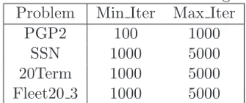
Thus, when the algorithmic reaches Min Iter, the apparent stability of the iterate is checked. If it appears to be stable, then the bootstrap-based optimality test is initiated. If the algorithm does not produce a solution that passed the optimality test by Max Iter, it simply terminates. The settings of these parameters varied with the problem dimensions as follows:

Table 2: SD Parameter Settings Problem Min Iter Max Iter

PGP2 100 1000

SSN 1000 5000

20Term 1000 5000

Fleet20 3 1000 5000

Of course, a primary computational difference between LSD and RSD is a result of the master program. LSD uses a linear master program, identical to the master program used in Benders’

Decomposition, except for the difference in the way that the cutting plane approximation of the recourse function is defined via the argmax procedure. The RSD objective is identical to the LSD objective, except for the addition of the term ¹₂(x−x)¯ ^>(x−x) (here, ¯¯ x is an “incumbent”

solution). Other than this quadratic term in the objective the LSD and RSD master programs are structurally identical. Of course, the trajectory of points identified by LSD and RSD will differ, which can impact the overall effort required to identify a solution.

In order to provide a basis for comparisons of the impact of master program, we compare the following performance measures:

• Objective Function Value – the value of the objective function associated with the solution identified upon termination. For PGP2, this value is calculated precisely. For 20Tterm, SSN, and Fleet20 3, this value was estimated based on independently generated observations and is accurate to within 1% with 95% confidence.

• Iterations required– the total number of iterations undertaken prior to termination.

• Time required – total “clock time” elapsed prior to termination of the algorithm.

We note that the solution methods in question use randomly generated data in their search for a solution. For this reason, we used 30 sets of runs (i.e., 30 different sequences of randomly generated observations). A single initial seed for our random number generator was used for each set, which ensures that LSD and RSD receive the same sequence of observations. Additionally, objective value estimation was undertaken with a single stream of observations, generated independently from the 30 streams used in the solution process. In this way, regardless of the master problem form (e.g., linear or regularized) and the run-time parameter settings (e.g., Min Iter, Max Iter, ²), the algorithms were exposed to identical sequences of observations in a controlled setting. As a result, differences in the output are due solely to the run-time settings that are under our control.

(10)

All programs were written in C, using the CPLEX callable library to execute master- and subproblem optimization (CPXbaropt was used to solve the RSD master program). The programs are run on a Sunw Sun-Fire-280R with 2xUltraSPARCIII processors at 900 MHz and 4GB of RAM and a Solaris 9 operating system. The machine used is a multi-user machine. Although efforts were made to ensure a dedicated computing environment, we cannot verify if, in fact, we were successful in this regard.

3.3 Results

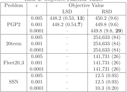
We begin by examining the quality of the solutions obtained by the various methods. In Table 3 below, the objective values associated with the various solutions obtained are listed. The tabulated values represent averages over 30 independent replications at each of the indicated settings of ², followed by the standard deviation associated with these 30 values in parentheses. In some cases, the method did not terminate prior to the maximum number of iterations permitted. In such cases, the objective values were averaged over the subset of runs which terminated as a result of having passed the optimality test and the number of such runs appear in boldface within the parentheses.

Thus, for example when solving 20term with ²= 0.001, the average estimated objective value for the 30 replications involving RSD was 254,632 and the standard deviation was 84.0. All of these runs terminated prior to reaching the maximum iteration count. A “–” is used to indicate that none of the 30 replications resulted in termination based on the optimality test (i.e., termination occurred when Max Iter was reached).

Table 3: Objective Function Values

Problem ² Objective Value

LSD RSD

0.005 448.2 (0.53, 13) 450.2 (9.6) PGP2 0.001 448.2 (0.54,7) 449.8 (9.6)

0.0001 – 449.8 (9.8,29)

0.005 – 254,633 (84)

20term 0.001 – 254,633 (84)

0.0001 – 254,633 (84)

0.005 – 141,731 (26)

Fleet20 3 0.001 – 141,731 (26)

0.0001 – 141,731 (26)

0.005 – 12.5 (0.93)

SSN 0.001 – 12.5 (0.93)

0.0001 – 10.3 (0.20)

There are several items worth noting in Table 3. First, we note that the optimal objective value for PGP2 is 447.32. It is interesting to observe that in general, the solutions identified were nearly optimal, but there is evidence of error. The standard deviations of the solutions’ objective value estimates are lowest with LSD (Stochastic Decomposition with a linear master program), but they exhibited a much stronger tendency toward reaching the maximum iteration count without

(11)

satisfying the termination criterion. On the other hand, RSD (Stochastic Decomposition with a regularized master program) exhibited a much larger standard deviation. Closer inspection of the specific objective values obtained indicates that this is due to a single run which terminated based on the optimality test, but identified a rather poor solution (with an objective value of 500.6).

When that particular run is omitted, the performance on this measure is similar to the other values reported. Of course, one accepts the possibility of error when using statistical estimates and randomly generated data. Note that within our termination criteria, we set α= 0.05 – indicating an acceptance of error beyond the specified level 5% of the time. In that sense, it is not surprising to see such error in one of the 30 runs undertaken.

The problem PGP2 is the smallest instance that we included in this test. It is small enough to be solved exactly using the L-Shaped method, which probably makes it the least interesting problem to discuss. The other three problems are sufficiently large as to preclude precise solution. It is interesting to note that in all of these problems, LSD was consistently unable to terminate prior to reaching the maximum iteration count, while RSD exhibited the exact opposite behavior – it terminated via the optimality tests in every single case. The solution values were remarkably stable – especially for the problems 20term and Fleet20 3, for which ²did not impact the solution. The problem SSN is anecdotally held to be among the most challenging two-stage SLPs available. We note that RSD terminated in every case, and the solution quality improved as the optimality error tolerance (i.e., ²) was reduced.

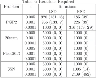
It is interesting to note the number of iterations required by the various methods prior to termination, as summarized in Table 4 below. The entries correspond to the average number of iterations over the 30 replications, followed by the standard deviation parenthetically. As in Table 3, we have also recorded the number of times that the methods terminated prior to reaching the maximum iteration count in boldface after the standard deviation. Thus, for example for ²= 0.001, solving PGP2 with LSD required 956 iterations on average, with a standard deviation of 133 and only 7 of the 30 replications terminated prior to the maximum iteration count. For the larger problems, the optimality test was never undertaken prior to reaching the maximum iteration count with LSD.

This phenomenon was observed with ²= 0.005, and our experimental set up ensured that it would also be observed with ²∈ {0.001,0.0001}. For this reason, we did not undertake these runs with the tighter tolerances.

Again we note distinct differences between the two versions of SD, especially on the larger problems. While the linear master exhibits a clear tendency toward failing to satisfy the termination criteria within the allotted number of iterations, the regularized master exhibits the exact opposite behavior and exhibits a clear tendency toward satisfying the termination criteria very early on (e.g., as soon as it was permitted to undertake the test!). Notable exceptions to this tendency appear with PGP2, in which there is clearly some variability in the number of iterations required to pass the termination criteria (which occurred in all cases), and SSN with the tight error tolerance of

² = 0.0001. These exceptions illustrate the adaptive nature of the method – the tests permit a recognition of insufficient evidence of solution quality to warrant termination. When that occurs, iterations continue until such evidence is obtained. Given the high degree of consistency in both the objective values and the iterations required for the regularized SD to solve 20term and Fleet20 3, it is likely that the Min Iter setting was higher than necessary.

(12)

Table 4: Iterations Required

Problem ² Iterations

LSD RSD

0.005 920 (15113) 185 (39) PGP2 0.001 956 (133, 7) 226 (39)

0.0001 1000 (0, 0) 316 (159, 29) 0.005 5000 (0, 0) 1000 (0) 20term 0.001 5000 (0, 0) 1000 (0) 0.0001 5000 (0, 0) 1000 (0) 0.005 5000 (0, 0) 1000 (0) Fleet20 3 0.001 5000 (0, 0) 1000 (0) 0.0001 5000 (0, 0) 1000 (0) 0.005 5000 (0, 0) 1000 (0) SSN 0.001 5000 (0, 0) 1005 (14)

0.0001 5000 (0, 0) 2409 (482)

We note that “iterations” alone are not sufficient for comparative purposes, as the “computational overhead” and the nature of the optimizations performed vary considerably. SD iterates with

“master problems” and “subproblems.” LSD works with a linear master program and RSD works with a regularized master program – a quadratic program, although the subproblems are identical in both cases. In order to reflect the impact that the form of the master problem might have, we also look at the time required to execute the algorithms through termination.

Table 5: Computational Times

Problem ² Time

LSD RSD

0.005 12.33 (16.48) 0.96 (0.35) PGP2 0.001 9.12 (9.14) 1.26 (0.48) 0.0001 5.74 (6.49) 2.67 (3.10) 0.005 25,644 (1235) 259.42 (31.94) 20term 0.001 25,644 (1235) 259.27 (31.90) 0.0001 25,644 (1235) 259.30 (31.85) 0.005 40,286.3 (943) 291.67 (2.54) Fleet20 3 0.001 40,286.3 (943) 291.67 (2.54) 0.0001 40,286.3 (943) 293.57 (2.45) 0.005 20,424 (8,127) 391.81 (17.05) SSN 0.001 20,424 (8,127) 341.70 (88.53) 0.0001 20,424 (8,127) 7491.81 (3728.67)

In Table 5, we summarize the computational time required to obtain these solutions. Again, we report the averages over 30 independent replications, with standard deviations reported parenthetically. The “time” recorded is the actual number of seconds required (i.e., the “wall clock”).

One immediately notices that RSD requires considerably less time than LSD on all problems. The average times reported were smaller, as were the standard deviations. We have already noted that

(13)

LSD often runs all the way to the maximum number of iterations allowed, which has an obvious impact on the time required. On the other hand, RSD terminates well before this limit is reached.

Additionally, RSD affords a more streamlined method for estimating error bounds. The added effort required to solve the quadratic master program (beyond that required for the linear master program) is more than compensated for by the reduced number of iterations required and the simplified termination criteria available.

It is interesting to compare the manner in which time/effort is allocated among the various computational activities by the two versions of SD. The primary computational requirements are:

• master program solution

• subproblem solution

• argmax-related computations (see Higle and Sen [1996])

• optimality tests (i.e., termination criteria)

• other “overhead” activities

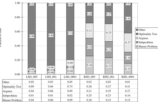
Figures 1-4 illustrate the allocation of time among these various activities for each problem instance.

Within these graphs, the type of master program used, linear or regularized, is indicated by the terms “LSD” and “RSD”, respectively. Since the value of ² varied, it is also reflected. Thus, for example, LSD 001 indicates solution with a linear master program using ² = 0.001, while RSD 0001 indicates a regularized master program with ²= 0.0001. Table 5 clearly indicates that LSD requires considerably more time than RSD for all problems – Figures 1-4 indicate how this time is distributed among the various activities. Note for example that Figure 1 indicates that when solving PGP2 with LSD the vast majority of the time is allocated to the optimality test (74%

- 89%, depending on the value of ² used). Indeed, the potential for extreme computational effort toward this undertaking was noted in§2. That this time is reduced somewhat as²is reduced results from the fact that given our run-time settings, a tighter error tolerance will also serve to prevent some tests from occurring (i.e., the preliminary test is also tied to this value of²). Because so much time is spent on the optimality test, it is difficult to appreciate the magnitude of the effort required for the remaining tasks. However, we note the computations required to perform the “argmax”

procedures are comparable to the time allocated to the master problem solutions. This remains approximately true when PGP2 is solved with the regularized master where substantially less time

(14)

Figure 1: PGP2 Time Allocations

0.04 0.06 0.09

0.26 0.23 0.01 0.01 0.15

0.02

0.25 0.23

0.16

0.04 0.06

0.09

0.21 0.25

0.27 0.89 0.84 0.74

0.26 0.27

0.41

0.02 0.03 0.05 0.02 0.02 0.01

0.00 0.20 0.40 0.60 0.80 1.00

Fraction of time Other

Optimality Test Argmax Subproblem Master Problem

Other 0.02 0.03 0.05 0.02 0.02 0.01

Optimality Test 0.89 0.84 0.74 0.26 0.27 0.41

Argmax 0.04 0.06 0.09 0.21 0.25 0.27

Subproblem 0.01 0.01 0.02 0.25 0.23 0.16

Master Problem 0.04 0.06 0.09 0.26 0.23 0.15 LSD_005 LSD_001 LSD_0001 RSD_005 RSD_001 RSD_0001

Figure 2: 20term, Time Allocations

0.01

0.23 0.23 0.23

0.00

0.20 0.20 0.20

0.84

0.50 0.50 0.50

0.00

0.06 0.06 0.06

0.15

0.01 0.01 0.01

0.00 0.20 0.40 0.60 0.80 1.00

Fraction of Time Other

Other 0.15 0.01 0.01 0.01

Optimality Test 0.00 0.06 0.06 0.06

Argmax 0.84 0.50 0.50 0.50

Subproblem 0.00 0.20 0.20 0.20

Master Problem 0.01 0.23 0.23 0.23

LSD RSD_005 RSD_001 RSD_0001

(15)

Figure 3: Fleet20_3, Time Allocations

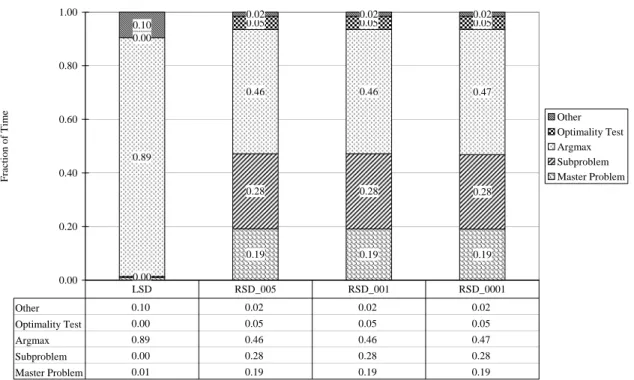
0.01

0.19 0.19 0.00

0.28 0.28 0.28

0.89

0.46 0.46 0.47

0.00

0.05 0.05 0.05

0.10

0.02 0.02 0.02

0.19 0.00

0.20 0.40 0.60 0.80 1.00

Other 0.10 0.02 0.02 0.02

Argmax 0.89 0.46 0.46 0.47

Subproblem 0.00 0.28 0.28 0.28

Master Problem 0.01 0.19 0.19 0.19

LSD RSD_005 RSD_001 RSD_0001

Figure 4: SSN, Time Allocations

0.04

0.51 0.48

0.00 0.10

0.06 0.06

0.01 0.75

0.32

0.31

0.38 0.00

0.09 0.14

0.50 0.20

0.02 0.02 0.01

0.00 0.20 0.40 0.60 0.80 1.00

Other 0.20 0.02 0.02 0.01

Argmax 0.75 0.32 0.31 0.38

Subproblem 0.00 0.06 0.06 0.01

Master Problem 0.04 0.51 0.48 0.10 LSD RSD_005 RSD_001 RSD_0001

(16)

is spent on optimality tests. Given that RSD is considerably faster than LSD in the first place, it appears that a substantial reduction in effort required to accomplish the optimality test has been accomplished, as suggested in §2.

In all of the other instances solved, LSD failed to undertake an optimality test due to the preliminary tests that were in place. In 20term, SSN, and Fleet20 3, we note that LSD allocates most of its effort toward the argmax computations (75-89%). In contrast, RSD spends a smaller fraction of time on these activities (31-50%). Given the variety of problem size statistics reported in Table 1, the effort required to solve the master and subproblems varies among the problems, as one expects.

4 Computational Investigation: Adaptive vs. Nonadaptive Solu- tion Techniques

In§3 we explore the computational impact of the error bound-based termination criteria described in §2. In this section, we explore the computational impact of the adaptive/internal sample-based technique, SD, to the nonadaptive/external sample-based technique, SAA. Recall that unlike SD which potentially considers a large sample size within a single run (if necessary), SAA proposes to solve a fixed number of instances (M), each with a fixed sample size (n). Given that our goal is comparative, we selectM andnso that SD and SAA use approximately the same observations per run.

To do this suppose that SD terminates in iteration K, indicating that a total of K observations were used to identify the solution. For each ofM ∈ {1,2,5,10}, we setn_M =K/M – rounding up if necessary to ensure that allM representations of SAA use the same number of observations within each replication of our experiment. Thus, for example, if SD terminates with K = 2557, then for M = 5, n₅ = d2557/5e = 512 while for M = 10, n₁₀ = 256. In this fashion, SD and SAA use essentially the same set of observations as they search for a solution to (1). In reporting our results, we refer to the process of usingM representations of SAA, each usingn_M observations as SAA M.

We note that SAA 1 is something of a misnomer. Without the replication formally required of SAA (see, e.g., Shapiro [2000]), SAA 1 is nothing more than the original problem instance in which the probability distribution is replaced by the empirical distribution associated with the observations generated in the course of the SD solution.

We use the term “SAA instance” to refer to the smaller stochastic program withn_M observations for some value of M. Thus, within any given “run”, we solve 1 SAA instance, with a sample size of n₁ =K, 2 SAA instances each with a sample size ofn₂, etc. Formally, SAA is a meta-method, because the SAA instances must still be solved. In our computations, all SAA instances were solved using Benders’ Decomposition (a.k.a., the L-Shaped method), and were terminated when the difference between the upper bound was within 0.0005, or when a maximum iteration count was reached. For PGP2, this maximum iteration count was set at 1000, and for the remaining problems, it was set at 4000. Recall that because SAA operates with a nonadaptive sample, the iteration count only controls the number of cuts used in the piecewise linear approximation of the

(17)

objective function. All of the results involving SD in this section were obtained with RSD, using

²= 0.0001. The minimum and maximum iteration counts for RSD were fixed as in Table 2 except for PGP2 for which Min Iter = 500 and Max Iter = 2000 were used.

Recall that SAA includes an intermediate step in which each of the M solutions obtained from a given SAA instance are evaluated so that the apparent best among them can be selected. Because the sample spaces associated with the problems under consideration are too large to permit precise objective function evaluations, these evaluations were undertaken with randomly generated data.

Whenever M >1, each of the SAA instance solution evaluations were performed with an independent set of observations, and are accurate to within 1%, with 95% confidence. For each value of M, the SAA instance solution with the minimum objective value estimate (based on this phase of independent posterior evaluation) is identified as the SAA solution.

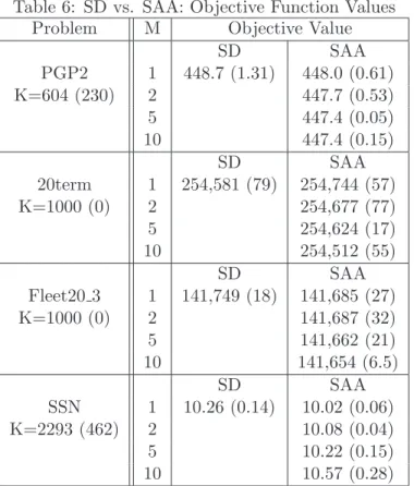
As in §3, we begin with a review of the objective values associated with the RSD and SAA solutions. In Table 6 below, we present the average objective values associated with the solutions obtained over multiple independent replications (10 for PGP2, and 5 for 20term, Fleet20 3, and SSN), with standard deviations reported parenthetically. As in Table 3, these objective values are exact for PGP2 and accurate to within 1%, with 95% confidence for 20term, Fleet20 3, and SSN.

Because it is an adaptive technique, “K” (the number of observations used by SD, and subsequently SAA) varied among the independent replications. For each problem, we report the average value of K, followed by the standard deviation (parenthetically).

Table 6: SD vs. SAA: Objective Function Values Problem M Objective Value

SD SAA

PGP2 1 448.7 (1.31) 448.0 (0.61)

K=604 (230) 2 447.7 (0.53)

5 447.4 (0.05)

10 447.4 (0.15)

SD SAA

20term 1 254,581 (79) 254,744 (57)

K=1000 (0) 2 254,677 (77)

5 254,624 (17)

10 254,512 (55)

SD SAA

Fleet20 3 1 141,749 (18) 141,685 (27)

K=1000 (0) 2 141,687 (32)

5 141,662 (21)

10 141,654 (6.5)

SD SAA

SSN 1 10.26 (0.14) 10.02 (0.06)

K=2293 (462) 2 10.08 (0.04)

5 10.22 (0.15)

10 10.57 (0.28)

(18)

There are several observations to make regarding Table 6. We will examine the output on a problem by problem basis, in combination with Figures 5-8 which illustrate the computational times required by the various methods.

PGP2:The average objective values obtained are all within 0.3% of each other. We note that RSD exhibits the highest average value as well as the largest standard deviation. Examination of the individual output indicates that as before, the high standard deviation associated with these values is due to a single run in which a high objective value (452.2) is obtained. On a run by run basis, the source of the maximum observed objective value was evenly divided between RSD and SAA 1, while the source of the minimum observed objective value was most often associated with SAA 5.

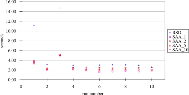
Figure 5 illustrates the time required to execute the solution of PGP2 with the various methods, for each of the 10 independent replications. In general, solutions were obtained within 4 seconds, regardless of the method used. However, two replications required considerably more with RSD (11.2 and 14.7 seconds). The non-adaptive method, SAA, appears to be well suited for this small problem.

20term:As far as objective values are concerned, all methods performed equally well. In addition to the averages being close and standard deviations being small, as indicated on Table 6, the difference between the minimum and maximum observed values is only 0.1%. Given that the values are only accurate to within 1% with 95% confidence, there are no discernible differences among the objective values obtained. Figure 6 illustrates the times required by the various methods to obtain their solutions. We note that because the differences are so extreme, it is necessary to view these times on a logarithmic scale. With regard to computational times, RSD exhibits a clear advantage. The times required by SAA are fairly stable across the four implementations tested and are nearly 1.5 orders of magnitude larger than the times required by RSD.

Fleet20 3: As with 20term, the objective values obtained in all cases are within 0.1% of each other, indicating that there are no discernible differences among them. Figure 7 illustrates the times required to obtain solutions. Again, the differences in these times are extreme, and again we see that the SAA solution times are nearly 1.5 orders of magnitude larger than for RSD.

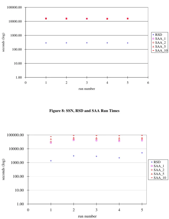
SSN:For this particular instance, SAA 1 exhibits the best objective value. That is, simply replacing the original distribution with the empirical distribution obtained from the observations generated during the course of the RSD runs produced the best objective values on average (and the least variable values as well). In all cases, the worst objective values obtained are associated with SAA 10. Figure 8 illustrates the solution times required. Again, SAA requires approximately 1.5 orders of magnitude more time to solve SSN than RSD. Unlike the other large problems (20term and Fleet20 3, which exhibited fairly stable solution times), SSN exhibits greater variation in times attesting to its reputation as a difficult problem. We note that even on this logarithmic scale, there is a clear discrepancy among the SAA solution times, with SAA 1 (Benders’ decomposition applied to the empirical distribution without the required SAA replications) considerably faster than the remaining SAA implementations. It would appear that in combination with the improved objective value estimates that it provides, among the various SAA runs tested, SAA 1 appears to be best suited for this particular instance. We note that this requires nearly 13 times longer to obtain a solution than SD, whose objective value is on average only slightly larger than the statistical error.

(19)

Figure 5: PGP2, RSD and SAA Run Times

0.00 2.00 4.00 6.00 8.00 10.00 12.00 14.00 16.00

0 2 4 6 8 10

run number

seconds

RSD SAA_1 SAA_2 SAA_5 SAA_10

Figure 6: 20term, RSD and SAA Run Times

1.00 10.00 100.00 1000.00 10000.00 100000.00

0 1 2 3 4 5

run number

seconds (log)

(20)

Figure 7: Fleet20_3, RSD and SAA Run Times

1.00 10.00 100.00 1000.00 10000.00 100000.00

0 1 2 3 4 5 6

run number

seconds (log) RSD

SAA_1 SAA_2 SAA_5 SAA_10

Figure 8: SSN, RSD and SAA Run Times

1.00 10.00 100.00 1000.00 10000.00 100000.00

0 1 2 3 4 5

run number

seconds (log)

(21)

Problem M Time

Solve Evaluate

PGP2 1 2.40 (1.08) 0 (0)

2 2.38 (1.03) 0.14 (0.01) 5 2.21 (1.00) 0.34 (0.01) 10 2.16 (0.83) 0.68 (0.02) 20term 1 11,757 (816) 0 (0)

2 11,189 (717) 4.42 (0.18) 5 11,547 (213) 11.15 (0.38) 10 11,851 (224) 22.77 (0.94) Fleet20 3 1 15,934 (340) 0 (0)

2 15,833 (408) 1.48 (0.05) 5 15,658 (228) 3.78 (0.09) 10 15,378 (272) 7.32 (0.16) SSN 1 36,893 (5,962) 0 (0)

2 37,627 (6,976) 7,989 (660) 5 39,100 (4,842) 21,146 (785) 10 46,340 (4,901) 41,792 (2,381) Table 7: SAA Time Allocations

It is clear that for all but the smallest problem, the SAA solution times are substantially higher than the SD solution times with approximately 1.5 orders of magnitude difference in all cases. Vari- ation in the SD solution times are attributable to the adaptive nature of its termination conditions, as we have discussed in §3. The source of the variation in the SAA solution times, especially as observed in SSN is less clear. Consequently, we examine the time allocated to each of the major computational requirements associated with SAA. Recall from §2 that SAA involves two major computational steps. GivenM, the number of SAA replications undertaken, it is necessary to

• solve M SAA instances of the problem (i.e., where the actual distribution is replaced by an empirical distribution) to obtain the set of M proposed solutions, and

• evaluate the objective function value associated with each of theM proposed solutions.

Following this, the proposed solution with the smallest objective function value estimate is selected as the SAA solution. In Table 7, we tabulate these times for each problem. “Solve” refers to the time required to solve the set of M SAA instances and “Evaluate” refers to the time required to evaluate theM proposed solutions. The numbers reported are averages over the 5 replications (ten replications for the smaller problem, PGP2) followed by standard deviations parenthetically. Note that in all cases, the evaluation time associated withM = 1 is identically 0 – in the absence of the SAA replications, there is no need to evaluate the proposed solution.

Examining the SAA time allocations provided in Table 7, the explanation behind some of our earlier observations becomes apparent. First, note that in general there is only limited variation

(22)

in the solution times as M varies from 1 to 10. That is, for these problem instances, it appears that the actual solution time is not critically dependent on the manner in which the observations are divided. While the number of observations naturally influences the solution times required, the manner in which they are distributed among the SAA instances does not in general. The exception to this is SSN, where we observe a fairly steady increase in the solution time required as M increases. Second, we note that two of the test problems, 20term and Fleet20 3 require relatively minimal time to evaluate the objective function values. Clearly, as M increases the time required to evaluate the proposed solutions increases as well. However, in these two problems, the time required to evaluate these solutions is negligible compared to the solution times required. On the other hand, evaluating the objective function values associated with the solutions to SSN is a more arduous undertaking. As M increases, the evaluation time becomes comparable to the solution time.

As a final comment, our benchmarking comparisons between SD and SAA are based on the L- Shaped method, so that there is a common algorithmic root shared by the solution methodologies.

We note that the L-Shaped method may not provide the most efficient solution procedure for the solution of the SAA instances. In order to understand the extent to which this might have been a factor in the extreme disparity in the solution times that we observed, we undertook a cursory investigation of alternative solution methods. In general, as one expects, we observe that for smaller sample sizes, CPLEX can solve the SAA instances faster than the L-Shaped method. This does not tend to be the case with the larger sample sizes, where the L-Shaped method can be considerably faster than CPLEX. That is, in contrast to our implementation of the L-Shaped method, where the manner in which observations are distributed among the SAA instances does not, in general, have an appreciable impact on the overall solution times, CPLEX is considerably faster with the smaller sample sizes than with the larger ones. We note that our observations in this regard apply only to the solution times, and not to the intermediate step in which all of the SAA instance solutions objective values are estimated. Additionally, we note that our observations regarding the relative performances of the linear and regularized versions of SD suggest that improvement in the solution of the SAA instances might also be obtained using a regularized L-Shaped method, as in Ruszczyński [1986]. Although we did not code a regularized L-Shaped method, we may look to the literature for results on comparisons based on a well-tuned implementation. Ruszczyński [1993], and Ruszczyński and ´Swietanowski [1997] provide numerical results with SSN using linear and regularized versions of the L-Shaped method, suggesting that the regularized version is approximately 3-4 times faster than the non-regularized version. This observation is based on a sample size of 200 observations, which approximately corresponds to the size of the SAA 10 instances for this problem (and of course, this excludes the intermediate function evaluation required by SAA). Thus, while in some cases the SAA instances may be solved faster using something other than the L-Shaped method, it appears that the regularized SD solution times are still faster, especially when the objective function evaluation requirements are taken into account.

(23)

5 Conclusions

Our computational results indicate fairly clearly that the regularized version of SD, with its more streamlined optimality tests, is more efficient than SD with a linear master program. The matrix computations associated with RSD’s optimality tests are less demanding than the replicated master program solution associated with LSD’s optimality tests. Combined with apparent differences in the solution trajectories (as indicated by the substantial differences in the number of iterations required), the additional computational effort required to solve the quadratic master program appears to be easily offset. With a small problem, such as PGP2, the differences in solution times are fairly minor, but with larger problems the differences are dramatic. It would appear that RSD prefers a tighter tolerance in its termination requirements, as the solution values appear to be less variable when this tolerance is tightened.

It appears that SAA may be well suited to the solution of the smaller problem. It exhibits an edge over RSD in the computational times, and in the objective values as well. In this particular case, M=1 does not perform as well as larger values of M. For all other instances tested, SAA requires substantially longer to obtain solutions than does RSD. Indeed, the differences in solution times are dramatic enough to require display with logarithmic scale, although this requirement would probably be lessened by an alternate choice of solution method for the SAA instances. In general, the differences in the objective values obtained are well below the statistical error associated with their estimated values, although this is not the case uniformly. In the more challenging problem (SSN), there is a preference for simply using M=1, which bypasses SAA and uses an empirical distribution with the largest sample size available. As a general rule, the need to evaluate objective function values for all M proposed solutions is an obvious computational bottleneck, although problems with relatively easy objective function evaluations pose less of a burden in this regard.

Although our intent was to investigate differences in the computational behavior of a method that exploits adaptive sample sizes (SD) with one that uses non-adaptive samples (SAA), we note that our experimental design offered SAA an opportunity to take advantage of information regarding sample sizes learned by SD in its adaptive setting. That is, the samples to which SAA was exposed were determined a priori by SD. Guidance on sample sizes can be found in Shapiro et al. [2002].

These sample sizes tend to be much larger than those that we have used, which will naturally serve to increase the computational times required. Additionally, the effort required to determine these sample sizes can also be somewhat extensive (requiring, for example, the expected value and variance of directional derivatives at optimal solutions). Of course, the impact of SD’s adaptive sample sizes is evident in the variable number of iterations and times required as it adjusts to the different sample paths to which it is exposed. The stability in the objective values produced by the RSD solution indicates some success in this adaptation. To be sure, there are cases in which there is variability in the objective values produced (most notably with PGP2), although this variability appears to be consistent with the statistical nature of the termination conditions imposed.

As a final comment, we lament the paucity of challenging test problems for experiments such as this! We note that we are necessarily restricted to three problems of meaningful magnitude and complexity (20term, Fleet20 3, and SSN), one of which is new! It is difficult to draw far reaching

(24)

comparisons and conclusions with so few meaningful test problems. As a result, we have restricted our observations to those that are blatantly obvious based on our computations, and hope that this state of affairs is remedied before too long.

Acknowledgement: This work was supported by Grant No. DMS 04-00085 from The National Science Foundation.

(25)

References

Benders, J. F. (1961). Partitioning procedures for solving mixed variables programming problems.

Numerische Mathematik 4, 238–252.

Birge, J. R. and F. V. Louveaux (1988). A multicut algorithm for two-stage stochastic linear programs. European Journal of Operational Research 34, 384–392.

Efron, B. (1979). Another look at the jackknife. Annals of Statistics 7, 1–26.

Higle, J. L. (2005). http://www.sie.arizona.edu/faculty/higle/Research/Data. as of April 2005.

Higle, J. L. and S. Sen (1991a). Statistical verification of optimality conditions.Annals of Operations Research 30, 215–240.

Higle, J. L. and S. Sen (1991b). Stochastic decomposition: An algorithm for two-stage linear programs with recourse. Mathematics of Operations Research 16, 650–669.

Higle, J. L. and S. Sen (1994). Finite master programs in stochastic decomposition. Mathematical Programming 67, 143–168.

Higle, J. L. and S. Sen (1996). Stochastic Decomposition: A Statistical Method for Large Scale Stochastic Linear Programming. Kluwer Academic Publisher.

Higle, J. L. and S. Sen (1999). Statistical approximations for stochastic linear programming problems. Annuals of Operations Research 85, 173–192.

Kleywegt, A. J., A. Shapiro, and T. Homem-de mello (2001). The sample average approximation method for stochastic discrete optimization. SIAM Journal on Optimization 12(2), 479–502.

Linderoth, J., A. Shapiro, and S. Wright (2002). The Empirical Behavior of Sampling Methods for Stochastic Programming. Technical Report 02-01, Computer Sciences Department, University of Wisconsin-Madison.

Mak, W. K., D. P. Morton, and R. K. Wood (1999). Monte carlo bounding techniques for deter- mining solution quality in stochastic programs. Operations Research Letters 24, 47–56.

Plambeck, E.L., F. B.-R. R. S. and R. Suri (1996). Sample-path optimization of convex stochastic performance functions. Math. Programming B 75, 137–176.

Ruszczy´nski, A. (1986). A regularized decomposition method for minimizing a sum of polyhedral functions. Mathematical Programming 35, 309–333.

Ruszczy´nski, A. (1993). Regularized decomposition of stochastic programs: Algorithmic techniques and numerical results. Working Paper WP-93-21, International Institute for Applied Systems Analysis, Laxenburg, Austria.

Ruszczy´nski, A. and A. ´Swietanowski (1997). Accelerating the regularized decomposition method for two stage stochastic linear problems.European Journal of Operational Research101, 328–342.

(26)

Sen, S., R. D. Doverspike, and S. Cosares (1994). Network planning with random demand.Telecom- munications Systems 3, 11–30.

Shapiro, A. (1991). Asymptotic analysis of stochastic programs. Annals of Operations Research 30, 169–186.

Shapiro, A. (2000). Stochastic programming by monte carlo methods. Available at:

www.isye.gatech.edu/ ashapiro/publications.html.

Shapiro, A., T. H. de Mello, and J. Kim (2002). Conditioning of convex piecewise linear stochastic programs. Mathematical Programming 94(1), 1–19.

Van Slyke, R. and R. J.-B. Wets (1969). L-shaped linear programs with applications to optimal control and stochastic programming. SIAM Journal on Applied Mathematics 17, 638–663.