Oil and Gas Markets
Inauguraldissertation zur
Erlangung des Doktorgrades der
Wirtschafts- und Sozialwissenschaftlichen Fakult¨ at der
Universit¨ at zu K¨ oln
2015
vorgelegt von
Diplom Volkswirt Benjamin Tischler aus
Burglengenfeld
Korreferent: Prof. Dr. J¨ org Breitung
Tag der Promotion: 2.Oktober 2015
First and foremost, I would like to express my gratitude to my supervisor, Assistant Professor Van Anh Vuong, Ph.D. for supporting my dissertation project. I greatly appreciated her constructive criticism and personal encouragement which strongly contributed to the success of this thesis. I would also like to thank Prof. Dr. J¨ org Breitung for his helpful methodological feedback and his encouragement to bring out the best in my research projects.
I am also grateful to Prof. Dr. Marc Oliver Bettz¨ uge for his inspiring ideas as well as for assuming the role of the chair of the examination committee for this thesis. Furthermore, I would like to thank my co-author Sebastian Nick for the productive and cordial work on our research project on the integration of gas market. Moreover, I feel indebted to Hans Manner for his great collaboration in our joint research on robust estimation and testing for market integration.
I would like to extend my gratitude to Niyaz Valitov, Meltem Kaplan and Leonie Hass who provided excellent research assistance. In addition, I would like to thank (in alphabetical order) Dimitri Dimitropoulos, Christian Growitsch, Felix H¨ offler, Erin Mansur, Anne Neumann and Luis Orea as well as Heike Wetzel for valuable comments and discussions on some of the essays included in this thesis.
Furthermore, I would like to express my gratitude to the Chair of Energy Economics and the Institute of Energy Economics at the University of Cologne (EWI) for providing an inspiring research environment and offering financial support for the participation in academic conferences. I am particularly grateful to Chris Sch¨ afer and Monika Deckers for her pervasive support during my time at Chair of Energy Economics and the EWI. The same applies for the whole administrative, communication, and IT-support team at EWI.
Finally, I would like to thank my family and friends for their support and encouragement. Above
all, I would like to thank Manuela for her love, inspiration and perennial support.
1 Introduction 1
1.1 Background and Motivation . . . . 1
1.2 Outline of the Thesis . . . . 3
2 What Drives Oil and Gas Drilling? A SVAR Approach to Supply Response 6 2.1 Introduction . . . . 6
2.2 Background . . . . 8
2.3 Data . . . . 11
2.4 Structural VAR Models for Oil and Gas drilling . . . . 13
2.5 Results . . . . 21
2.5.1 Impulse Response Functions and Forecast Error Variance Decompositions . . 21
2.5.2 The Drivers of Oil and Gas Drilling Activity . . . . 23
2.5.3 How Oil and Gas Prices Respond to Shocks in Oil and Gas Drilling . . . . . 28
2.6 Conclusions . . . . 30
i
3.1 Introduction . . . . 32
3.2 Theoretical Framework . . . . 35
3.2.1 The Law of One Price and its Application to Global Natural Gas Markets . . 35
3.2.2 Econometric Approach . . . . 38
3.3 Empirical Application . . . . 40
3.3.1 Data . . . . 40
3.3.2 Threshold Estimation and Testing for (Threshold) Cointegration . . . . 41
3.3.3 TVECM Estimation - Adjustment of Individual Prices . . . . 45
3.3.4 General Discussion . . . . 48
3.4 Conclusion . . . . 50
4 Robust Testing of the Law of One Price in Natural Gas Markets 52 4.1 Introduction . . . . 52
4.2 Methodology . . . . 54
4.2.1 Testing for Spatial Arbitrage . . . . 54
4.2.2 Robust Estimation of Threshold Autoregressions . . . . 56
4.3 Monte Carlo Study . . . . 57
4.3.1 Small Sample Biases . . . . 57
4.3.2 Critical Values and Power of Cointegration Tests . . . . 60
4.4 Application to US and UK Natural Gas Prices . . . . 61
4.5 Conclusion . . . . 63
ii
5.1 Introduction . . . . 65
5.2 The Shale Revolution and the Role of Experience Curves . . . . 67
5.2.1 The Shale Revolution as a Result of Growing per Rig Production . . . . 67
5.2.2 Drilling Productivity and the Role of Technology and Experience . . . . 69
5.3 Theoretical and Empirical Model . . . . 70
5.3.1 Empirical Model . . . . 70
5.3.2 The Role of Drilling Technology and Technology Specific Experience . . . . 73
5.4 Estimation Strategy . . . . 74
5.5 Data . . . . 76
5.6 Results . . . . 77
5.7 Conclusion . . . . 81
A Supplementary Material for Chapter 2 83 B Supplementary Material for Chapter 4 87 B.1 Monte Carlo Alternative Specifications: Bias and Power for BAND-TAR models . . 87
B.2 Monte Carlo Alternative Specifications: Bias and Power for EQ-TAR models . . . . 89
C Supplementary Material for Chapter 5 92
Bibliography 93
iii
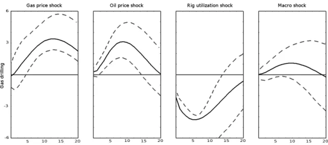
2.1 Responses of gas drilling activity in the gas model . . . . 24
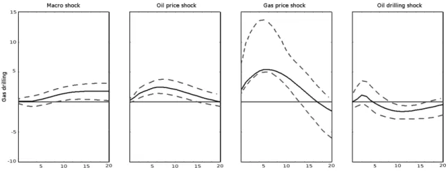
2.2 Responses of gas drilling activity in the joint model . . . . 25
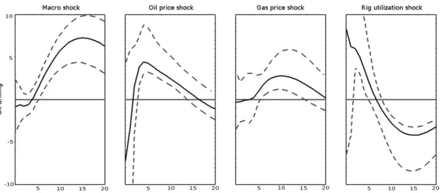
2.3 Responses of oil drilling activity in the oil model . . . . 26
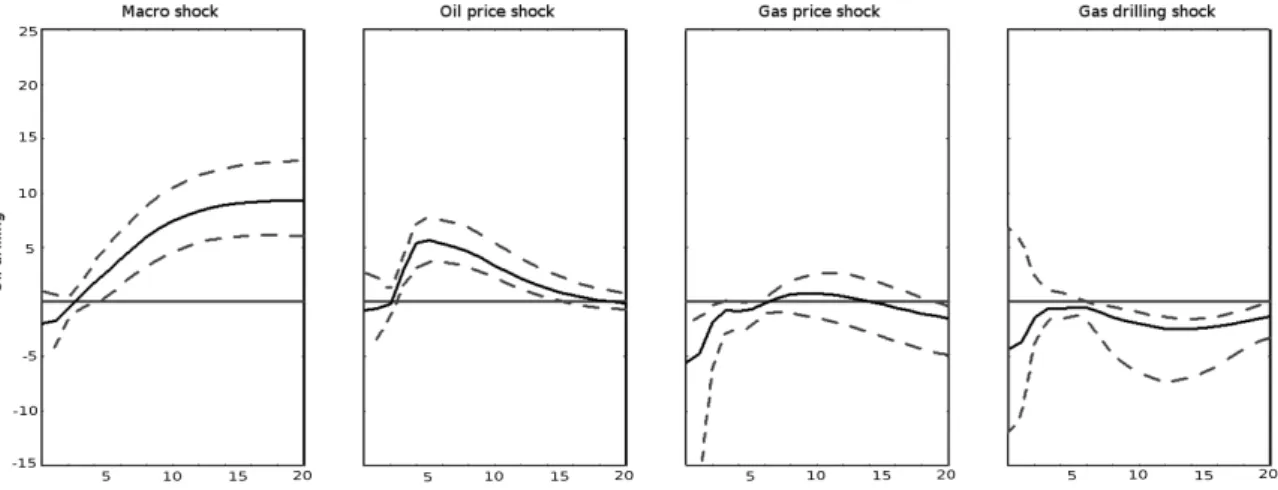
2.4 Responses of oil drilling activity in the joint model . . . . 27
2.5 Responses of gas price in the joint model . . . . 28
2.6 Responses of the oil price in the joint model . . . . 29
3.1 Price Difference between UK National Balancing Point and US Henry Hub . . . . . 33
3.2 Regional Price Arbitrage in the Global Natural Gas Market . . . . 37
3.3 Prices for UK National Balancing Point (Solid Line) and US Henry Hub (Dashed Line) 49 4.1 BAND-TAR: Bias in threshold estimates (left) and power of cointegration tests (right) in the base specification . . . . 58
4.2 EQ-TAR: Bias in threshold estimates (left) and power of cointegration tests (right) in the base specification . . . . 59
4.3 Price spreads of US and UK gas markets . . . . 61
4.4 Potential threshold values τ and the value of the objective function for the OLS, t-ML and LAD estimators. . . . 63
5.1 US total and shale production of crude oil and natural gas. Source: US Energy Information Administration . . . . 68
5.2 Average initial production per drilling rig. Source: US Energy Information Adminis- tration . . . . 68
A.1 Oil and gas drilling activity [Number of Rigs] 1993-2012 . . . . 84
A.2 Real oil and gas price [normalized to Jan 1993 = 100] 1993-2012 . . . . 84
A.3 Macroeconomy 1993-2012 . . . . 85
A.4 Rig utilization rate 1998-2012 . . . . 85
iv
ADF Augmented Dickey-Fuller test
ARCH Autoregressive conditional heteroscedasticity BAND-TAR Band threshold autoregressive model
BAND-TVECM Band threshold vector error correction model
BH Baker Hughes
CCEMG Common correlated effects mean group estimator CCEP Common correlated effects pooled estimator EIA US Energy Information Administration EQ-TAR Equilibrium threshold autoregressive model FD First difference estimators
FE Fixed effects estimator
FEVD Forecast error variance decomposition FGLS Feasible generalized least squares estimator
GDP Gross domestic product
HH Henry Hub
HQ Hannan-Quinn Information Criterion
IRF Impulse Response Function
JB Jarque-Bera residual normality tests LAD Least absolute deviations
LL Log-likelihood
LM Lagrange Multiplier
LNG Liquefied natural gas
LOP Law of One Price
LR Likelihood ratio
LTC Long term contract
MA Moving average
MMBtu Million British thermal units NBP National Balancing Point OLS Ordinary least squares estimator
SAR Sum of the absolute values of the residuals SC Schwartz Information Criterion
SER Sequential elimination of regressors procedure SSR Sum of squared residuals
TAR Threshold autoregressive model
v
UK United Kingdom
US United States of America
WTI West Texas Intermediate
vi
Introduction
1.1 Background and Motivation
Since the 1960s hydrocarbons like crude oil and natural gas have been the most important energy source to fuel the world economy. Despite high recent growth rates for renewable energies, hydro- carbons are expected to be a dominant source of energy for several decades to come. In the last 20 years not only fundamental trends, but also singular events such as the financial crisis have shaped the development of crude oil and natural gas markets as well as the corresponding academic debate.
On a historic scale these last two decades have seen changes in oil and gas markets that - in terms of price and regional production changes - are only matched by the turmoils of the oil crisis of the 1970s. Hence, the objective of this thesis is to improve the understanding of some of the dynamics and trends underlying these developments.
Around the turn of the millenium the growth of wealth and resource consumption in emerging economies and the fear of shrinking oil and gas production in industrialized countries refueled the time-honored debate about the point of time when the supply of fossil energy resources will reach its historic all time high. Labeled as the “peak oil hypothesis” the discussion gained most momentum for the case of crude oil, but similar worries were also expressed for natural gas. These solicitudes were also reflected and amplified by prolonged and steep increases in global oil and gas prices which in turn raises the question of how strong hydrocarbon supply will react to these price shocks. Accordingly, Chapter 2 of this thesis addresses oil and gas supply response to oil and gas price changes in the US. More specifically, because oil and gas supply can only be kept constant or increased by drilling additional wells, the essay focuses on the response of oil and gas drilling activity to changes in oil and gas prices as well as drilling costs.
1
In the late year 2008 the oil and gas price boom came to a sudden end in a stark collapse during the turbulences of the financial crisis and its macroeconomic aftermath. Both oil and gas prices stopped plummeting only in spring 2009. Whereas global oil prices quickly recovered to pre-crisis levels, the US price of natural gas stayed at low levels and even started to trend slightly downward. Given the growing gas prices in Europe this led several market stakeholders to announce a disintegration of the Atlantic gas market into an US market and an European market. However, given quickly expanding transport capacities and trade volumes for liquified natural gas (LNG) other industry participants hesitate to consent with the market decoupling hypothesis. Accordingly, Chapter 3 empirically investigates the integration of Atlantic gas markets before and after the financial crisis.
Price spikes are a frequent phenomenon in natural gas and other commodity markets. This can result in a low power of empirical market integration tests that are based on threshold autoregressive models. Similarly, threshold autoregressive (TAR) model based estimates of the transaction costs of arbitrage can be subject to large small sample biases when extreme price movements are present.
To address this Chapter 4 investigates the small sample properties of TAR estimators and TAR based market (co-)integration tests. To remedy the poor small sample properties of the usual OLS based TAR estimation we propose two robust estimators. Accordingly, Chapter 4 methodologically advances the econometric approaches used in Chapter 3.
In North America, the major driver underlying this putative gas market decoupling was the so called shale revolution - a term that describes a steep and unforeseen increase in hydrocarbon supply from unconventional shale formations in the US. The shale revolution started off in gas markets where the novel combination of hydraulic fracturing and horizontal drilling in formerly unfamiliar shale geology enabled sweeping production gains. However, oil drilling also quickly adopted the new approach.
By tapping shale oil resources with cost-efficient technologies and pulled by high oil prices US crude
oil production is now close to surpassing its historic all time high of November 1970. Hence, for the
moment the advent of the US shale revolution has refuted most arguments for an impending now
and forever peak in US oil or gas production. As shale resources are available in many countries
around the globe, the success of the US shale revolution stimulates the desire to replicate the shale
revolution in other countries. A large part of the technical side of the replication debate is about
updating the technology of rig fleets such that they are capable of performing hydraulic fracturing
and horizontal drilling. However, in the US industry participants also highlight the importance
of accumulated experience in using these technologies in a given region. Against this background,
Chapter 5 investigates the role of drilling technology and local drilling experience as drivers of the
oil and gas production growth during the US shale revolution. When the accumulation of local
experience plays a crucial role for shale oil and gas production, it might be difficult to replicate the
shale revolution in other countries by merely updating the technology level of the old rig fleet.
1.2 Outline of the Thesis
This thesis comprises four empirical essays on the economics of crude oil and natural gas markets.
The following paragraphs briefly outlines the background, research questions, the methodological framework and the findings of the four essays.
Chapter 2 “What Drives Oil and Gas Drilling? A SVAR approach to supply response” investigates supply response in US crude oil and natural gas markets by disentangling the drivers of oil and gas well drilling activity. Further, the feedback from drilling activity on oil and gas prices is addressed.
Since the turn of the millennium, the dramatic changes in crude oil and natural gas prices on the one hand and US oil and gas production on the other hand stress the question of how oil and gas supply react to price changes. Oil and gas production crucially depend on how many new oil and gas wells are drilled in order to replace the declining production of older oil and gas wells. For this reason, market stakeholders have a great interest in understanding how well drilling activity reacts to changes in oil and gas prices and drilling cost. Another reason for this interest is that drilling activity statistics are published with very little delay to real time. Thus, drilling activity data can be regarded as the earliest available, reliable indicator for medium term changes in oil and gas supply.
Prior studies such as Ringlund et al. (2008) either focused on oil drilling or gas drilling activity.
However, oil drilling activity is interrelated with and gas drilling activity in at least two ways. First, the costs of oil and gas drilling are interdependent because the same drilling rigs are used for oil and gas wells. Moreover, oil wells often produce a significant amount of gas (and vice versa for natural gas wells). Thus, the revenues of both oil and gas wells are dependent on oil and gas prices.
To account for these interrelations between oil and gas drilling a structural vector autoregressive (SVAR) model is employed to disentangle the drivers of oil and gas drilling activity. In addition, the SVAR model is used to investigate whether changes in drilling activity feed back on oil and gas prices. The results imply that gas drilling is both driven by expected revenues - represented by gas and oil prices - and drilling cost. In contrast, oil drilling activity is mainly driven by variables related to the expected revenues, namely oil prices and macroeconomic activity. Whereas gas prices are strongly affected by changes in drilling activity, oil prices seem to react to drilling activity only weakly in the medium term.
Chapter 3 “The Law of one Price in Global Natural Gas Markets - A Threshold Cointegration
Analysis” investigates market integration between the US and the European market for natural gas
before and after the finacial crisis. In the latter period declining US gas prices led to a debate about
whether or not the US and the European gas markets are still interlinked by liquefied natural gas
(LNG) arbitrage. The essay is a joint work with Sebastan Nick, who equally contributed to all parts of the study as co-author.
In the last decade, trade volumes of liquefied natural gas have expanded largely and are thought to indicate a trend towards a stronger integration of natural gas markets around the world. According to the Law of one Price (LOP) we expect prices of a homogenous good such as natural gas to converge under such circumstances. In contrast, important benchmark prices of natural gas around the globe seem to have decoupled since the financial crisis in the year 2009 and since the US shale revolution gathered momentum. Against this background, we empirically investigate whether the LOP holds even if prices seem to wander far from each other. In specific, we focus on the relationship between the prices at the Henry Hub in the US and the National Balancing Point in the UK. Previous research such as Neumann (2009) mostly used linear cointegration approaches to study the subject matter. However, linear approaches ignore that there should be no arbitrage activity, i.e., no error correction when the price difference is smaller than the transaction costs of arbitrage. First, we improve on the existing literature by using a threshold autoregressive (TAR) framework that is more adequately capturing the dynamics of spatial arbitrage in gas markets by explicitly taking account of transaction costs. Second, we use our model to test for market (co-)integration and to estimate a measure of transaction costs. Third, we investigate the adjustment of UK and US gas prices using a threshold vector error correction model. Our empirical results reveal a stable long-run relationship with threshold error-correction dynamics for the period 2000-2008 and for the period 2009-2012 when gas prices seem decoupled. However, in the latter period we find evidence for substantial impediments to arbitrage that by far exceed the usual US-UK transport cost differential.
Further, for the period 2000-2008 we find that price convergence occurred by adjustment in both the US and UK market. In contrast, since the year 2009 price convergence was mainly achieved by downward pressure on the high UK prices.
Chapter 4 “Robust testing of the law of one price in natural gas markets” investigates the small sample performance of TAR based estimates of the transaction costs of arbitrage and related tests for market integration when price series are contaminated with price spikes. As a remedy for the weak small sample performance of OLS based methods two robust procedures for TAR based transaction cost estimation and testing for market integration are proposed. Hans Manner co-authored the study, and contributions to all aspects of the essay were made in equal parts.
Threshold auto-regressive models can be used to test for market integration in accordance with the
law of one price as well as to estimate the transaction costs of arbitrage between two connected
markets. However, resource and commodity price series such as natural gas frequently exhibit
temporary price spikes. Interpreted as outliers or fat tails, such extreme price movements may
lead to poor sample properties of TAR estimates and related cointegration tests. Particularly, price spikes may result in a large small sample bias in TAR threshold parameter estimates, representing transaction costs, and in a low power of to market (co-)integration tests. Hence, this paper considers the robust estimation of transaction costs using TAR models and robust testing of the LOP in the presence of occasional extreme price movements. We use Monte Carlo simulation and an application to US and UK natural gas prices to demonstrate that, in the presence of fat-tails or outliers OLS based estimates of the threshold, i.e., the transaction cost parameter can be severly biased. This, in turn, leads to a lower power of TAR based cointegration tests for market integration. In order to mitigate these problems, we propose two robust TAR estimation procedures based on the least- absolute-deviations (LAD) estimator and the maximum likelihood estimator assuming t-distributed errors (t-ML). The Monte Carlo simulations show that in the presence of fat tails or outliers the robust estimators have a lower small sample bias regarding the threshold parameter than the OLS estimator. Moreover, the our robust cointegration tests for market integration have a higher power than OLS based tests when fat tails or outliers are present.
Chapter 5 “The Role of Experience for the Shale Revolution” investigates the role of local experience and drilling technology for the US shale revolution.
“Hydraulic fracturing” and “horizontal drilling” are without doubt the core technologies behind the sweeping rise of US oil and gas production during the shale revolution. Additionally, industry repre- sentatives often stress the importance of experience for oil and gas extraction from shale formations.
More specifically, local experience, i.e., the part of overall experience which cannot spill over to other regions or countries seems to play a decisive role in the shale industry. Furthermore, a strong role of local experience has implications for a replication of the shale industry in other countries. Whereas the technology level in other countries can be adjusted to US levels by upgrading the drilling rig fleet, local experience has to be accumulated by a large number of drilling operations. This in turn, would make it even more difficult for other countries to catch up on the US shale revolution.
Against this background, this essay empirically investigates the role of both drilling technology
and local drilling experience for the production of shale oil and gas. To address this, we estimate
oil and gas production functions that account for drilling technology and drilling experience. To
take account of experience spillovers and to identify the effect of local drilling experience, we use
the common correlated effects mean group estimator (CCEMG) and the pooled common correlated
effects (CCEP) estimator introduced by Pesaran (2006). We find robust evidence for strong local
experience effects in shale oil and gas production. Further, by disaggregating drilling and experience
into different technology classes we can confirm that horizontal drilling indeed contributes most
to the production of shale oil and gas. Moreover, the impact of experience gathered by using the
horizontal drilling technology has the largest impact on shale oil and gas production compared with
other production factors.
What Drives Oil and Gas Drilling?
A SVAR Approach to Supply Response
2.1 Introduction
Around the turn of the millenium the growth of wealth and resource consumption in emerging economies and the fear of shrinking oil and gas production in industrialized countries refueled the time-honored debate about the point of time when the supply of fossil energy resources will reach its historic all time high. Labeled as the “peak oil hypothesis”, the discussion gained most momentum for the case of crude oil, but similar worries were also expressed for natural gas. The upsurge in the peak oil and gas debate coincided with shrinking US oil and gas production as well as with substantial increases in both global oil prices and US natural gas prices. However, in the years around 2005 gas production in the US started to grow again and US oil production followed this turnaround with a short delay. After a strong downturn during the financial crisis in the late year 2008, domestically determined US gas prices stayed on low levels. In contrast, globally determined oil prices quickly recovered almost to pre-crisis levels. On a historic scale, the movements of hydrocarbon prices during the first decade of the new millenium are only matched by the oil price movements of the 1970s oil crisis. These dramatic changes in crude oil and natural gas prices on the one hand and US oil and gas production on the other hand stress the question of how oil and gas supply react to price changes.
In the medium term, oil and gas production crucially depend on how many new oil and gas wells are drilled in order to replace the declining production of older oil and gas wells.
1Therefore,
1 “Medium term” refers to reactions in a variable that need between a few weeks and several months to take place after a shock in a driver of that variable has occurred.
6
market stakeholders who are interested in medium term supply response have a great interest in understanding how drilling activity reacts to changes in oil and gas prices and drilling cost. Another reason for this interest is that drilling activity statistics are published with very little delay to real time. Thus, drilling activity data can be regarded as the earliest available, reliable indicator for medium term changes in oil and gas supply. Accordingly, the main objective of this essay is to empirically investigate how the development of US oil and gas drilling activity is interrelated with the movement of oil and gas prices. We also address the role of drilling costs for oil and gas drilling activity. Further, because drilling activity is the most important early indicator of future supply, prices may react to changes in drilling activity. Hence, we also investigate whether changes in oil and gas drilling activity feed back on oil and gas prices. Finally, oil and gas prices as well as oil and gas supply may depend on overall economic activity in the US. Therefore, we also account for the state of the US economy in our analysis.
Up to now there are only few empirical studies on supply response in oil and gas extraction in general and drilling in particular. Studies on drilling responses start with an early work by Renshaw (1989) who employs a simple regression analysis to estimate the effect of an oil import fee on drilling activity in the USA. Iledare (1995) estimates the response of drilling measured as total footage drilled for natural gas to changes in wellhead prices and other variables. He uses pooled cross-sectional data for 1977 to 1987 for West Virginia. Ringlund et al. (2008) estimate price elasticities of oil drilling for different world regions and find that the US have a comparably high long-run price elasticity of oil drilling of 1.2 percent. Ringlund et al. (2008) use a bivariate autoregressive distributed lag model. Due to low data availability, they only include prices and drilling activity in their model and try to capture all other influences on drilling activity with deterministic regressors as well as with a stochastic time trend. Boyce and Nostbakken (2011) derive a theoretical model to explain exploratory and development drilling in the very long run. The model is tested using random and fixed effects estimators and a panel of US states with yearly observations from 1955 to 2002. A positive relationship between the number of drilled oil and gas wells and real oil and gas prices is found. The most recent paper in the field is Kellogg (2014) who uses monthly data from 1993 until 2003 and estimates the response of oil drilling in Texas to changes in the expected volatility of crude oil future prices.
Prior studies either focused on oil drilling or on gas drilling activity. However, oil drilling activity is
interrelated with gas drilling activity in at least two important ways. First, the costs of oil and gas
drilling are interdependent because the same drilling rigs are used for oil and gas wells. Moreover,
oil wells often produce a significant amount of gas (and vice versa for natural gas wells). Thus, the
revenues of both oil and gas wells are dependent on oil and gas prices.
To account for these interrelations, we use a structural vector autoregressive (SVAR) model to disen- tangle the drivers of oil and gas drilling activity. In addition, the SVAR model is used to investigate whether changes in drilling activity feed back on oil and gas prices. Further, the SVAR framework accounts for feedback between the variables that may lead to endogeneity problems in single equation approaches. Impulse response functions (IRF) and Forecast error variance decompositions (FEVD) are used to present and analyze the estimation results.
The results indicate that gas drilling is driven by variables that determine the revenues and by variables that determine the costs of gas drilling projects. In contrast oil drilling is mainly driven by variables that determine the revenues of oil drilling projects. Oil prices are only weakly affected by changes in oil drilling activity, whereas gas prices respond strongly and instantaneously to shocks in gas drilling activity. The remainder of this essay is organized as follows. In Section 2, the economics of the US oil and gas drilling are discussed. Section 3 presents the data. In section 4 the econometric approach is discussed, the SVAR models are specified and the identification approach is explained.
In section 5 the SVAR estimates are presented and section 6 concludes.
2.2 Background
This section explains the technological and institutional setting in which oil and gas drilling activity take place and discusses the potential medium term drivers of drilling activity. Hydrocarbons such as crude oil and natural gas are extracted from fields i.e. underground geological formations that store hydrocarbons. Oil and gas production firms extract, process and sell oil and gas. Extraction is preceded by the exploration of a field by seismic surveys and scattered wildcat drilling to obtain some knowledge about the expected well output and the necessary drilling effort.The exploration phase is succeeded by the field development phase. In the development phase a great number of wells is drilled with the objective to profitably extract oil and gas for processing and sale. According to conversations with industry participants drilling processes last between a few weeks and many months - depending on geological characteristics and corresponding technological challenges.
2Even given the geological field information available from the exploration phase, there is still some uncer- tainty left about the output and necessary drilling effort of development wells. Completed oil and gas wells exhibit high initial production rates which subsequently decline at decreasing rates due to the loss of geological pressure on the emptying reservoir.
Exploratory and development drilling in the US is sometimes conducted by the oil and gas production firms themselves, but more often realized by independent drilling companies.
3Accordingly, drilling
2 In the definition used here, the drilling process starts when the borehole is spud and ends when the well is completed.
3 See Kellogg (2011) for details on the cooperation of drilling companies and production companies.
is often not an integral part of the activity of production companies, but there exists a leasing market for drilling rigs where suppliers are independent drilling companies and demanders are production companies. The costs of new wells, but also the total upstream costs of oil and gas production companies consist mainly of drilling cost.
4Other upstream costs that occur after a well was drilled such as land lease, maintenance or pumping cost are very low in comparison. Whether or not a potential well with certain technological and geological characteristics is drilled is therefore mostly determined by expected drilling costs and expected revenues from the well. Hence, drilling activity should react to changes in expected revenues i.e. expected oil and gas prices as well as changes in expected drilling cost.
Expected revenues from drilling a well are determined by expected gas and oil prices over the total lifespan of the investment. Hence, the question arises how drilling investors form their expectations of future oil and gas prices. At least three possibilities seem sensible. First, future or forward prices could be used as predictors of expected spot prices in the future. However, according to Hamilton (2009) and Farzin (2001) future prices have theoretical as well as empirical drawbacks. Generally, future prices are not ideal predictors for spot prices in the future because they typically include costs of carry and risk premia. The latter could be positively correlated with the behaviour of current spot oil and gas prices as increased spot price volatility might lead to higher risk premia.
Consequently, future prices may have weak predictive power especially in the volatile gas market.
Second, following the theory of rational expectations (Muth 1961) current spot prices should already include all available information about future market development that is presently available. Hence, current spot prices could be used as a proxy for expected future prices. Third, the formation of price expectations could be adaptive i.e. market participants expect prices in the future to be a weighted average of current and past spot prices. Farzin (2001) argues that the adaptive version is also useful because it smoothes out short-run price volatility. The practical disadvantage of the adaptive expectations approach is that the number of time periods over which the average is calculated is arbitrary.
In this study the rational expectations approach is followed and current gas and oil spot prices are used to proxy expected future prices. Correspondingly, changes in drilling activity and resulting changes in expected oil and gas production might also have an instantaneous impact on oil and gas spot prices. In contrast to many other countries, in the US drilling statistics are published with only a few days delay to real time. Hence, drilling statistics are the earliest available, reliable indicator of future US production and supply of oil and gas. Accordingly, market participants are very vigilant about drilling statistics. Changes in drilling activity may, therefore, have an effect on buy and sell decisions in oil and gas trading which in turn influences the oil and gas price.
4 The upstream part of the oil and gas sector is defined here as starting with the drilling of oil and gas wells and ends with the wholesale of extracted and processed oil and gas.
However, the response of US natural gas prices to changes in drilling activity can be expected to be stronger than the response of oil prices. The majority of US natural gas consumption is covered by domestic gas production. Hence, gas prices are mainly influenced by US domestic production and consumption. In contrast, the share of US domestic oil production in US oil consumption is smaller compared to natural gas. Moreover, the oil price is closely linked to global oil market developments and the condition of the overall US economy. Hence we expect the feedback from gas drilling to gas prices to be larger than the feedback from oil drilling to oil prices.
An important aspect of the revenue side of drilled wells is that they often produce both crude oil and natural gas in proportions that depend on field characteristics. Thus, registering a drilling project e.g. as a “gas drilling project” only means that the most of the revenues are expected to be generated by natural gas. But, in many gas fields oil or associated hydrocarbons such as ethane, propane, butane or natural gasoline can be found which are priced close to crude oil or natural gas prices depending on their specific characteristics. Hence, oil prices may also play a role for the revenues of declared “gas wells”.
5The same argument makes gas prices relevant for the revenues of oil wells. Therefore, in an empirical analysis of the determinants of oil or gas drilling activity both oil and gas prices have to be considered as explanatory variables.
Not only expected revenues, but also expected drilling cost are among the determinants of drilling activity. The costs of drilling projects can typically be fixed or at least quite precisely estimated at the point of time when the decision to realize a drilling project is made.
6The costs of drilling a well are mainly determined by the geology, technology and drilling rig rental rates. Data on geological and technological determinants of drilling cost are hard to measure on an aggregate level and are not publicly available. The role of technology for aggregate drilling activity is ambiguous. On the one hand, technological progress can increase drilling activity when formerly inaccessible or unprofitable oil and gas deposits become accessible or profitable. On the other hand, technological progress can also decrease drilling activity as drilling projects can be finalized in shorter time. Both points are certainly true for unconventional drilling techniques such as hydraulic fracturing and horizontal drilling. In addition, Geology and the corresponding drilling technology change only in the long run. The objective of this essay, however, is to investigate the medium term determinants of drilling activity. Accordingly, we focus on the components of drilling costs that vary in the medium term.
5 In some world regions that concentrate on crude oil extraction the share of gas in oil wells is negligible and vice versa for some “gas regions”. However, in the US there is a substantial share of wells that deliver both gas and oil in economically significant amounts even if the wells are registered as “gas wells” or “oil wells”. This phenomenon is particularly prevalent for the case of unconventional oil and gas extraction.
6 Thus, uncertainties about drilling cost and expectation formation do not play a major role on the cost side of drilling projects.
Thus, we explicitly account only for rig scarcity and rig rental costs by using the utilization rate of the US rig fleet as a proxy for drilling cost.
7Exogenous factors that influence drilling activity include seasonal effects such as the spring thaw in northern US states that impedes the movement of heavy equipment and natural disasters such as the hurricane season in the year 2005 which lead to the temporary shut down of drilling activities.
Other determinants of drilling activity are labor availability and tax issues. Due to data constraints these determinants have to left unaccounted for. However, it seems unlikely that the omission of these variables creates important inconsistencies in the estimates as they are arguably not strongly correlated with the other explanatory variables used in the models below.
Finally, the empirical analysis is facilitated by the assumption of competitive upstream oil and gas markets in the US. The assumption is underpinned by the high number and the not too heterogeneous size of market participants in both the rig market as wells as the wholesale markets for oil and gas.
2.3 Data
Monthly observations covering the period from October 1998 to September 2012 are examined. Data with monthly frequency are adequate to study the medium term response structure of oil and gas drilling activity. This sample period starts well after the gas and oil markets had adapted to reforms and deregulation that took place in the late 1980s. The sample is also recent enough to include observations since the rise of unconventional oil and gas extraction.
Oil and gas drilling activity data are from the US Energy Information Administration (EIA) and originally from the Baker Hughes‘s North American Rotary Rig Count which is a monthly census of the number of onshore rigs actively drilling for oil or natural gas in the United States.
8The rig count is a very comprehensive measure of exploration and field development activity as it only excludes insignificant rigs such as very small truck mounted rigs, cable tool rigs and rigs that can operate without a permit. The real natural gas wellhead price for the US is used as the price of natural gas. Nominal wellhead prices were obtained from the EIA database and were deflated using the
7 Drilling rigs are usually used for both oil and gas drilling. Thus, the approximation of the medium term variation of oil and gas drilling cost by rig utilization rates is reasonable. In the estimation below, we alternatively use the amount of oil drilling activity as an approximation of the costs of gas drilling (and vice versa). The quality of this approximation approach depends on further assumptions, e.g. about the size of drilling rig fleet and its reaction to rig scarcity. Hence, this second approximation approach will only serve as a robustness check, when the drivers of oil and gas drilling activity are investigated.
8 “A rig is considered active from the moment the well is “spudded” until it reaches target depth [...]. Rigs that are in transit from one location to another, rigging up or being used in non-drilling activities [...] are not counted as active”. Drilling data are available at http://www.eia.gov/dnav/ng/ng˙enr˙drill˙s1˙m.htm.
monthly US implicit GDP deflator.
9Wellhead prices are calculated by dividing the total reported value of all sold gas at the wellhead by the total quantity produced as reported by the appropriate US agencies. Therefore, wellhead prices include all costs prior to shipment from the lease including gathering and compression costs, severance and similar charges, but exclude pipeline transmission costs which can be significant at least when the pipeline system reaches its capacity limit. Wellhead prices can be considered as spot prices, but adjusted for transmission costs associated with current pipeline capacity limitations. Therefore, the wellhead price is more closely related to the revenues of gas extraction companies than, say, the Henry Hub spot price. Still, wellhead prices closely follow the spot prices at the most liquid trading places such as the Henry Hub. However, wellhead prices experience softer spikes than are typically observed at the Henry Hub which is another reason for preferring wellhead prices when it comes to econometric model estimation.
The real free on board prices of the benchmark crude oil West Texas Intermediate (WTI) as traded at the Cushing-Oklahoma spot market are used as oil prices. The nominal WTI oil prices were obtained from the US Energy Information Agency (EIA) database and were deflated using the monthly US implicit GDP deflator
10. To proxy the costs of onshore rigs monthly rig utilization rates are obtained from the Guiberson-AESC Well Service Rig Count.
11Albeit the Guiberson-AESC rig count actually measures onshore oil rig utilization rates, it closely resembles rig utilization rates because as outlined above almost all rigs can be used for both oil and gas drilling. Rig utilization rates are measured as the percentage share of rigs that are actively drilling compared to the total number of available rigs in the market. A rig is considered as active if, on average, it is crewed and worked every day during the month. The monthly, seasonally adjusted industrial production index of the US Federal Reserve Database represents the situation of the overall US economic situation. It is used as driver of oil and gas demand and therefore serves as an additional proxy for expected oil and gas well revenues.
12The industrial production index measures the real production output of manufacturing, mining, and utilities and is standardized such that the average index values for the months of the year 2007 are equal to one hundred.
The Figures A.1, A.2, A.3 and A.4 in Appendix A show the plots of all time series used. Table A.1 and A.2 in the appendix provide detailed definitions, sources and descriptive statistics on the data and variables.
9 The monthly values for the implicit GDP deflator were obtained by linear interpolation of quarterly deflator values to a monthly frequency. The wellhead prices are available at http://www.eia.gov/dnav/ng/ng˙pri˙sum˙dcu˙nus˙m.htm and the gdp deflator is available at http://research.stlouisfed.org/fred2/series/GDPDEF/
10 WTI spot price are available at http://www.eia.gov/dnav/pet/pet˙pri˙spt˙s1˙m.htm
11 Available at http://www.c-a-m.com/Forms/Product.aspx?prodID=cdc209c4-79a3-47e5-99c2-fdeda6d4aad6
12 The US industrial production index is available at http://research.stlouisfed.org/fred2/series/INDPRO/
2.4 Structural VAR Models for Oil and Gas drilling
In this section the empirical approach to estimate the drivers of oil and gas drilling activity is pre- sented and corresponding econometric models are specified. Our approach also addresses how oil and gas drilling activity feeds back on oil and gas prices. The empirical analysis is based on the estimation of a system of dynamic simultaneous equations in the form of a structural vector autore- gressive model (SVAR). The SVAR is estimated in levels and identified by short run restrictions on the instantaneous relationships between the variables.
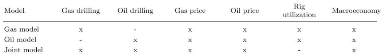
Table 2.1: Set of variables in the gas model, the oil model and the joint model
Model Gas drilling Oil drilling Gas price Oil price Rig
utilization Macroeconomy
Gas model x - x x x x
Oil model - x x x x x
Joint model x x x x - x
The “x” represents endogenous variables that are included in the respective model given in the left column. A “-”
means that a variable is not included in the model.
In order to provide robust results for the response of oil and gas drilling activity three models are specified. The first model focuses on the explanation of gas drilling activity ( gas model), the second model explains oil drilling activity (oil model ) and the third model aims at explaining both oil and gas drilling activity jointly (joint model). Moreover, the joint model is used to investigate how shocks in drilling activity affect oil and gas prices. Each model contains a different subset of the variables as shown in Table 2.1. Gas drilling and oil drilling is the number of onshore rigs actively drilling for oil and natural gas, respectively. Gas prices are real US natural gas wellhead prices and oil prices are real Western Texas Intermediate spot prices proxying expected future oil and gas prices.
The rig utilization rate is from the Guiberson-AESC data set and approximates drilling cost. The macroeconomy variable is the industrial activity index of the Federal Reserve Economic Data base and represents the overall economic situation in the US.
The gas and oil model include gas and oil drilling activity, respectively, as the dependent variables of
main interest. All three models proxy the expected revenues of gas and oil drilling, respectively, by
the oil and gas price as well as by the macroeconomy variable. In the gas model and the oil model
drilling costs are approximated by the rig utilitzation rate. In the joint model gas drilling activity is
used as a proxy for the cost of oil drilling and vice versa for the cost of gas drilling. With this latter
approach drilling costs can only be approximated roughly. Therefore, the joint model is only used
as a robustness check for the results on the drivers of oil and gas drilling obtained from estimating
the gas model and the oil model, respectively.
The joint model is primarily used to estimate how oil and gas drilling activity affect oil and gas prices. As oil and gas wells often produce both oil and gas, both oil and gas drilling are included in the joint model.
13Therefore, it is important to not only include variables representing oil and gas supply, but also variables representing oil and gas demand. Accordingly, the joint model contains oil and gas drilling as a measure of (expected future) supply of oil and gas. The macroeconomy variable as well as deterministic terms capturing seasonalities (explained below) serve as a rough measure of (expected future) oil and gas demand.
As several demand and supply side variables are missing in the joint model, it clearly cannot fully explain oil and gas price formation. Other supply side variables include net storage withdrawals as well as pipeline and overseas imports. The demand side is mainly determined by demand from electricity generation, transport, heating and industrial activity. However, these omitted demand and supply side variables are arguably not strongly correlated with oil or gas drilling activity in the short and medium term once macroeconomic activity and seasonality are accounted for in the joint model. Thus, the corresponding bias in the parameter estimates regarding price responses to shocks in drilling activity is arguably small.
The variables were tested for unit roots and cointegration.
14The unit root tests provide evidence that the variables are integrated of order one. Only the tests on the utilization rate are ambiguous.
Depending on the test specification utilization rates are sometimes positively sometimes negatively tested for unit roots. The full set and relevant subsets of the variables were tested for cointegra- tion. The tests were inconclusive about whether or not the variables are cointegrated. Gospodinov et al. (2013) discuss the advantages of alternative estimation approaches when there is uncertainty about the exact nature of (co-)integration. They conclude that unrestricted SVAR models that are estimated in levels and identified by short run restrictions are the most robust specification when tests are inconclusive about the magnitude of the largest roots and cointegration between the vari- ables. Moreover, any estimated cointegration relationships established with the variables at hand would lack a clear theoretical interpretability. Therefore a level SVAR model with restrictions on the instantaneous relationships between the variables is used as the basic specification.
The reduced form of all three models is specified with the help of maximum lag order selection as well as subset selection procedures and evaluated with diagnostic tests. Thereafter, a structural model is identified and estimated using restrictions on the instantaneous relationship between the
13 In contrast, the gas model and the oil model only contain gas drilling or oil drilling, respectively. Hence, these two models cannot take account of the fact that oil drilling activity may increase gas supply which in turn may affect gas prices. The same argument holds for gas drilling activity, its effect on oil supply and, eventually, oil prices.
14 The tests proposed by Elliott et al. (1996) and Kwiatkowski et al. (1992) were used to test for unit roots. The test proposed by Johansen (1988) and Johansen and Juselius (1990) was used to determine the cointegration rank.
Different lag orders and deterministic specifications were tested. The test results are left out here for brevity.
variables. All three models are based on a reduced form VAR model of order P that can be written as
y
t=
P
X
i=1
B
iy
t−i+ ΦD
t+ e
t(2.1)
where y
tis a N-dimensional vector of the endogenous variables presented in Table 2.1, the B
iare N × N coefficient matrices for the lags of y
t. Φ is a N × K matrix where K is the number of deterministic regressors. Further, e
tis a N-dimensional vector of reduced form errors which have a zero expected value E(e
t) = 0, have no autocorrelation E(e
te
0s) = 0 for all s 6= t but are allowed to be contemporaneously correlated E(e
te
0t) = Σ
e, that is, e
t∼ (0, Σ
e).
The capricious paths of drilling activity, utilization rates and natural gas prices (see Figures A.1, A.4 and A.2 in Appendix A) create problems with the normality of the residuals which leads to less precise estimates. Given our moderate sample size, influential outliers may distort the parameter estimates. To mitigate these problems, we include event dummy variables where there there are extreme residuals and where there is economic reason to do so. Hence, D
tis a vector of deterministic variables that includes impulse dummies for major events such as hurricanes and the downturn of the US economy during the financial crisis. Additionally, D
tcontains a time trend and seasonal dummies.
The time trend accounts for general technological progress. The seasonal dummies capture seasonal variations in oil and gas drilling as well as seasonal variations in oil and gas demand represented by oil prices, gas prices and the macroeconomy variable. To account for the trend shift after the economic crisis that is apparent in the drilling activity time series a trend shift variable is included that starts in May 2009.
15This point of time roughly corresponds with the time when the US shale revolution starts to gain momentum. Hence, by including a trend shift variable we take account of technological change associated with the US shale revolution. The trend shift dummy is put where the strongest downturns of the financial crisis have ended and where visual inspection of the oil drilling data strongly suggests a trend shift. Table A.3 in Appendix A gives a detailed overview over the deterministic regressors in the models.
First, for each of the three models the maximum lag order of the VAR system is determined using the Schwartz (SC) and Hannan-Quinn (HQ) information criteria.
16The SC and the HQ criteria point to a maximum lag length of two or three. A maximum lag length of three is choosen as specification tests detect no residual autocorrelation with this maximum lag order.
17Second, the large sets of
15 The trend shift variable is zero for all time periods before May 2009 and increases by one each month afterwards.
16 L¨utkepohl (2005) argues that the other alternatives for information criteria - namely the Akaike information criterion and the Final Prediction Error criterion - asymptotically overestimate the true VAR order, whereas the SC and HQ criteria offer consistent estimates of the true order.
17 Residual autocorrelation can be detected when a maximum lag length of only two is used.
regressors in the VAR models reduce the degrees of freedom for the estimation and would lead to too imprecise estimates when the full set of regressors was used. Therefore, the sequential elimination of regressors (SER) algorithm proposed by Br¨ uggemann and L¨ utkepohl (2000) is employed to further decrease the number of parameters in each of the three models by imposing subset restrictions on the reduced form VAR. The SER sequentially eliminates the lags of the explanatory variables that lead to the largest reduction of the selected information criterion until no further reduction is possible for the system of VAR equations. The remaining subset of regressors is deemed to include the most relevant regressors in statistical terms. In addition, Breitung et al. (2004) highlight that the asymptotics of SVAR estimates and the related impulse response functions are strongly improved when variables with a coefficient that is indeed zero are restricted to zero in the estimation. Third, the reduced forms of the three models are estimated with the SER subset restrictions in place using the feasible generalized least squares estimator (FGLS) outlined in L¨ utkepohl (2005).
18Diagnostic tests for residual autocorrelation and residual normality as well as tests for ARCH-effects are employed to evaluate the consistency and the efficiency of the estimates. Model checking results for all three models are shown in Table 2.2 (tests for residual autocorrelation) and in Table 2.3 (tests for residual normality and ARCH-effects).
Table 2.2: Tests for residual autocorrelation for the gas, the oil and the joint model
Test Qgas,16 LMgas,5 Qoil,16 LMoil,5 Qjoint,16 LMjoint,5
Test statistic 392.5 136.1 376.5 144.3 362.2 132.3
Appr. distrib. χ2(374) χ2(125) χ2(376) χ2(125) χ2(376) χ2(125)
p-value 0.24 0.23 0.48 0.11 0.68 0.30
Q16 and LM5 represent the Portmanteau and Breusch-Godfrey LM test for autocorrelation as described in L¨utkepohl (2004) for lag orders ofh = 16 and h = 5 for the gas, the oil and the joint model, respectively. In both cases the null hypothesis of no residual autocorrelation is tested against the alternative that at least in one residual series there is autocorrelation up to the specified lag order. The Brensch-Godfrey LM test has most power when testing for low orders of residual autocorrelation, whereas the Portmanteau test is preferable for large lag orders.
Most importantly, there is no evidence for autocorrelation in the residuals in all three models. There is some evidence for ARCH effects in some of the residuals in the oil and the joint model. Despite event dummy variables included there is still non-normality in some residuals of the oil and the joint model. Particularly, the residuals of the drilling and the utilization rate equations show ARCH effects and residual non-normality. The latter might be due to the fact that the sudden movements in drilling activity that produce extraordinarily high residuals cannot be fully captured by the event dummy variables. However, the inclusion of more event dummies is not considered as sensible as this would consume more degrees of freedom in the estimation and there is potentially too much arbitrariness involved when dummies are included for purely statistical reasons and without a strong
18 The reduced form estimates are not shown as they are of no interest in themselves due to their lack of economic interpretability.
Table 2.3: Tests for residual normality and ARCH-effects
Model JB Normality Gas
drilling
Oil
drilling Gas price Oil price Utilization rate
Macro- economy
Gas model Test statistic 21.8 - 3.79 6.74 59.9 2.04
p-value 0.00 - 0.15 0.03 0.00 0.36
Oil model Test statistic - 535.9 3.86 5.32 106.8 0.50
p-value - 0.00 0.14 0.06 0.00 0.77
Joint model Test statistic 5.14 150.2 6.16 3.20 - 0.31
p-value 0.07 0.00 0.04 0.20 - 0.85
Model ARCH-LM Gas
drilling
Oil
drilling Gas price Oil price Utilization rate
Macro- economy
Gas model Test statistic 14.6 - 15.8 15.1 13.8 11.8
p-value 0.26 - 0.19 0.23 0.31 0.45
Oil model Test statistic - 75.7 16.2 14.4 19.3 6.19
p-value - 0.00 0.17 0.27 0.08 0.90
Joint model Test statistic 12.4 78.3 16.4 14.6 - 13.8
p-value 0.40 0.00 0.17 0.26 - 0.31
Results for univariate Jarque-Bera (JB) residual normality tests and univariate ARCH-LM tests as described in L¨utkepohl (2004) are presented. The JB tests the null hypothesis of residual normality for one of the VAR equations.
The ARCH-LM test has the null hypothesis of no ARCH effects in any of the residual series up to the specified lag length. Here, ARCH effects are tested up to a lag order of twelve. The rows of the panel show the test statistic and the p-value for the gas model, the oil model and the joint model for the JB test in the upper part of the panel and for the ARCH-LM test in the lower part. The columns two to seven show the results for the residuals of the specific VAR equations.
economic argument. To summarize, the tests show that the model is not fully satisfactory in every regard. But despite some deficits in efficiency due to non-normality and ARCH effects the estimates can be still regarded as appropriate for the purpose of this study. As linear dependencies are analyzed in the form of impulse response functions and variance decompositions, the reduced form estimates can nevertheless be considered as an adequate basis for the subsequent estimation of the structural from of the VAR model.
The estimation of a reduced form model is already a statistically valid description of the data generating process. But a reduced form model can only be a starting point as it generally has no economic interpretation.
19To allow for an economic interpretation the corresponding structural form of the model has to be identified and estimated. In the structural representation instantaneous relations between some of the endogenous variables are allowed, but a sufficient amount of such relation has to be restricted based on economic intuition. That is, contemporaneous values of some endogenous variables are allowed as explanatory variables in some equations. The structural representation corresponding to equation 2.1 is given by
B
0y
t=
P
X
i=1
B
i∗y
t−i+ Φ
∗D
t+
t(2.2)
19 The reduced form VAR model particularly lacks economic interpretability when economic intuition or theory suggest instantaneous relations between the endogenous variables and when there is correlation between the reduced form errors.
where y
tis defined as in the reduced form versions of the three models. B
0is an invertible N × N coefficient matrix representing the instantaneous relations between the endogenous variables.
20The B
i∗are N × N matrices of structural coefficients where B
i∗= B
0B
i. Φ
∗is a N × K matrix of structural coefficients for determinstic regressors where Φ
∗= B
0Φ and
tis a N-dimensional vector of structural errors where
t= B
0e
t. A number of restrictions has to be imposed on the structural model to make the number of estimated structural parameters equal to the number of reduced form parameters. Ignoring deterministic terms in the reduced form model (N
2)P + 1/2[N
2− N ] param- eters are estimated. Again ignoring the determinstic terms and under the standard assumptions that structural errors are white noise and independently distributed and that the variances of the structural errors are normalized to one in the structural form (N
2− N) + N
2P parameters have to be estimated.
21Thus the difference in the number of parameters is 1/2(N
2− N). This is just equal to the number of additional restrictions that need to be imposed to identify the structural model.
In our case these restrictions are imposed as zero restrictions on the matrix of instantaneous rela- tions B
0. That means, using this identification scheme assumes that shocks may affect a subset of variables directly within the current time period, whereas another subset of variables reacts only after a time lag. An advantage of zero restrictions is that researchers can often find clear arguments for (not) imposing them based on economic intuition or theory. With arguably more responsive variables such as oil and gas prices on the one hand and presumably more laggard variables such as utilization rates, drilling and the macroeconomy variable on the other hand there should be enough pronounced differences in the (instantaneous) reaction patterns to make this identification scheme valid. Accordingly, with N = 5 endogenous variables for identification at least ten zero-restrictions have to be imposed on B
0.
22The identification schemes for the gas model, the oil model and the joint model are presented in the Tables 2.4, 2.5 and 2.6. Table 2.4 shows how the matrix of instantaneous impacts is restricted for the gas model which is mainly designed to explain the drivers of gas drilling activity. Drilling activity is allowed to instantaneously react to changes in all other variables. Even though large movements in drilling activity can only be expected in the medium term, i.e., with a lag of several weeks or months, drilling activity may still react very quickly to changes in its drivers. This can be due to idle drilling rigs that are already located in the large oil and gas regions in Texas and Louisiana and can be made operational in less than a month. This point is backed by Ringlund et al. (2008) who find an instantaneous reaction of drilling activity to price changes on a monthly basis. In contrast, prices
20 In its normalized version the diagonal ofB0 contains only ones. The matrix is normalized such that each row represents an equation where the variable with coefficient one is the dependent variable.
21 That is, the variance-covariance matrix of the structural errors is an identity matrix.
22 For just identification exactly 1/2(N2−N) = 1/2(52−5) = 10 restrictions have to be imposed. For over- identification more than ten restrictions have to be imposed. When more restrictions can be imposed than are necessary for just identification over-identification tests offer the possibility to test for the validity of the set of restrictions. This allows for potential statistical support for a certain choice of zero restrictions.
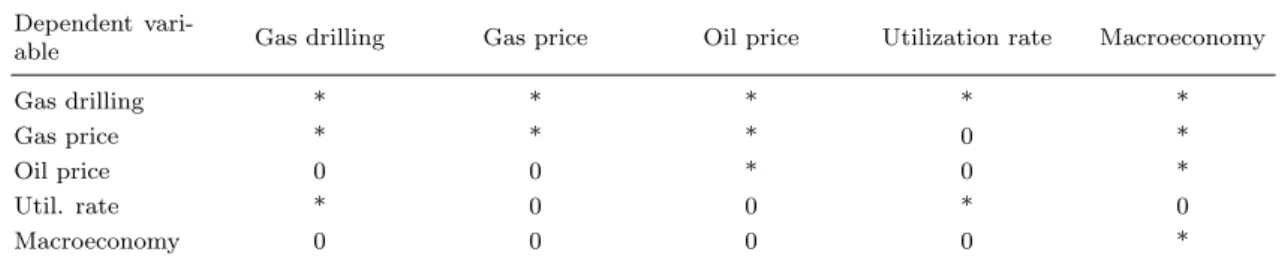
Table 2.4: Matrix B
0with identifying zero restrictions for the gas model
Dependent vari-
able Gas drilling Gas price Oil price Utilization rate Macroeconomy
Gas drilling * * * * *
Gas price * * * 0 *
Oil price 0 0 * 0 *
Util. rate * 0 0 * 0
Macroeconomy 0 0 0 0 *
Each row represents the coefficients of the instantaneous relationships between the endogenous variables of an equation in the system of VAR equations with the left column showing the dependent variable in that equation. An asterisk * means that the respective instantaneous relationship is estimated without restrictions. A zero means that a zero restriction is imposed on this instantaneous relationship.
are generally thought to have a fast reaction when new information about market fundamentals is available. Thus, gas prices are allowed to react instantaneously to gas drilling because drilling is perceived by market stakeholders as one of the most important and the most quickly available indicators of changes in future domestic US gas supply. Oil is a substitute for gas on the demand side in heating, the chemical industry and in electricity generation, hence, the gas price is allowed to instantaneously react to oil price changes. Similar to oil prices shocks to the US economy might also have a direct effect on gas prices because gas demand at least from electricity generation is strongly linked to overall output of an economy. Only the utilization rate is not allowed to have an instantaneous impact on the gas price. This is because almost any movement in the utilization rate that could have an instantaneous impact on the gas price is already captured by allowing for an instantaneous reaction of the gas price to shocks in gas drilling activity.
Oil prices are determined mainly by developments in the global market for crude oil of which the US economy is an important part. The impact of oil coming from gas wells and equally the impact of gas drilling activity on oil prices should be negligible in the very short run. The same is true for utilization rates proxying drilling cost which are most likely too remotely related to oil prices on a monthly basis. Hence, only the US macroeconomy is allow to influence oil prices instantaneously.
According to Ramberg and Parsons (2012) oil and gas prices are cointegrated, but whereas gas prices react to deviations from the long run relationship oil prices do not adjust to deviations. That is oil prices can be considered to “pull” the gas prices in the very short run, but not the other way around.
Due to this weak exogeneity property of oil prices gas prices are restricted to have no instantaneous impact on oil prices. Utilization rates naturally should react instantaneously only to drilling activity as the share of utilized rigs clearly changes with the number of rigs drilling for natural gas. However, the size of the rig fleet certainly cannot react to any influences in the short run.
Macroeconomic activity is assumed to feature no instantaneous reaction to any of the variables
which is supported by the fact that the energy sector constitutes only a small part of the overall
US economy. Any change in gas or oil prices - let alone rig utilization rates or gas drilling activity - should trickle down only slowly into the overall economic situation. The number of restrictions is therefore eleven.
23With eleven restrictions the model is overidentified by one restriction which offers the advantage that the validity of the identification scheme is testable. The LR Test as proposed in Breitung et al. (2004) for the validity of the overidentifying restriction uses a χ
2distribution with one degree of freedom and yields a test statistic of 0.0846 and a p-value of 0.77. Thus, the overidentification test does not reject the overidentifying restriction which can be seen as some additional statistical support for the identification scheme used here.
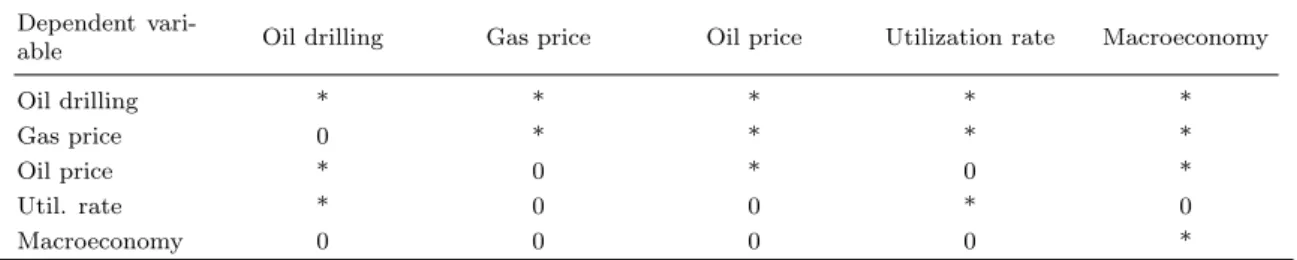
Table 2.5: Matrix B
0with identifying zero restrictions for the oil model
Dependent vari-
able Oil drilling Gas price Oil price Utilization rate Macroeconomy
Oil drilling * * * * *
Gas price 0 * * * *
Oil price * 0 * 0 *
Util. rate * 0 0 * 0
Macroeconomy 0 0 0 0 *
See notes for Table 2.4.
Table 2.5 shows the restrictions on the instantaneous relationships for the oil model. In the oil model drilling activity for crude oil is the variable of main interest. So, it is allowed to instantaneously react to all the other modeled variables. The gas price is allowed to instantaneously react to all variables, but oil drilling activity. This restriction is arguably valid as gas coming from oil wells is typically of minor importance for the overall US gas supply in the sample period. Further, as geological surveying is costly the amount of gas coming from oil fields and, thus, oil drilling is often not explored with equal precision as expected oil quantities. This uncertainty in how much additional oil drilling is contributing to gas supply and, eventually, gas prices might also decrease the instantaneous response of gas prices to oil drilling. Hence, it seems acceptable to restrict the instantaneous impact of changes in oil drilling activity on gas prices to zero. Oil price responses are restricted in the presented way for similar reasons as in the gas model. However, as the oil sector is the major focus of the oil model oil prices are allowed to react instantaneously to oil drilling activity.
As in the gas model utilization rates again only react to drilling activity and macroeconomic activity is considered exogenous within a one month time horizon.
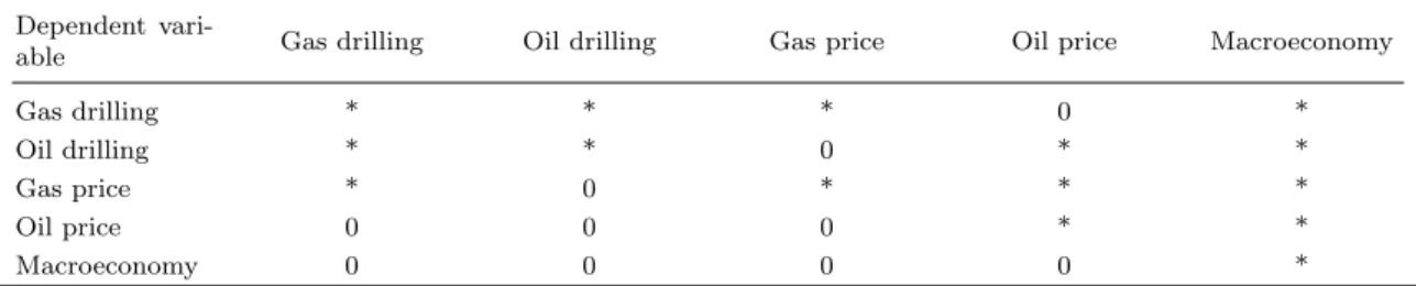
Table 2.6 shows the restrictions on the instantaneous relationships for the joint model. The joint model aims at incorporating the responses of both gas and oil drilling activity in one model and
23 Alternative just- and overidentified models were also estimated. The results in the most reasonable specifications were qualitatively the same. However, there was a small number of reasonable identification schemes where the estimation procedure - the scoring algorithm explained below - did not converge. The overidentifying restrictions used here are considered as the most credible restrictions among the models in which the algorithm converged.