Physics of Traffic on Ant Trails and Related Systems
I n a u g u r a l - D i s s e r t a t i o n zur
Erlangung des Doktorgrades
der Mathematisch-Naturwissenschaftlichen Fakult¨ at der Universit¨ at zu K¨ oln
vorgelegt von Alexander John
aus Leverkusen
K¨ oln 2006
Berichterstatter:
Prof. Dr. A. Schadschneider Prof. Dr. D. Stauffer
Tag der m¨undlichen Pr¨ufung:
8. Dezember 2006
Contents
1 Introduction. . . 1
1.1 Motivation . . . 1
1.2 Outline . . . 3
2 The ASEP and its Variants. . . 5
2.1 Definition . . . 5
2.1.1 Boundary Conditions . . . 6
2.1.2 Update Schemes . . . 7
2.2 The TASEP . . . 8
2.2.1 Models based on the TASEP . . . 13
2.3 The TASEP with Static Disorder . . . 18
2.3.1 Particlewise Disorder . . . 19
2.3.2 Latticewise Disorder . . . 22
3 The Unidirectional Model . . . 27
3.1 Definition . . . 27
3.1.1 Some Aspects Concerning Reality . . . 28
3.1.2 Exact Mapping to Other Models . . . 29
3.2 Properties of the Unidirectional ATM . . . 31
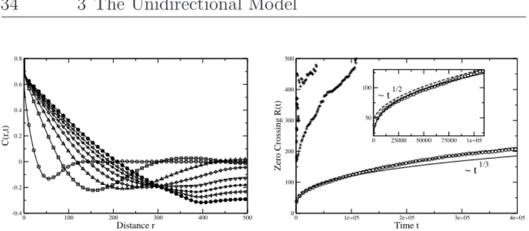
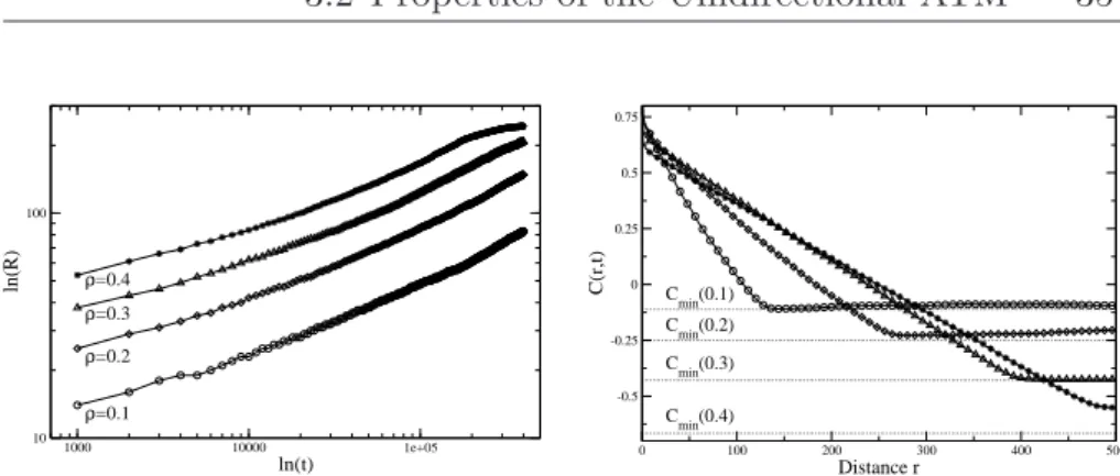
3.2.1 Observed Patterns . . . 31
3.2.2 Coarsening Behaviour . . . 32
3.2.3 The Stationary State . . . 35
3.3 Discussion . . . 38
4 The Bidirectional Models. . . 41
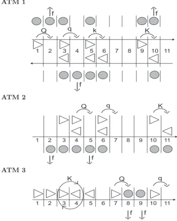
4.1 Definitions and Properties . . . 41
4.1.1 Bidirectional Trail with Separated Pheromone Lattices . . 43
4.1.2 Bidirectional Trail with Common Pheromone Lattice . . . 45
4.1.3 Single-lane Bidirectional Ant Trail Model . . . 47
4.2 Common Features . . . 51
4.2.1 Moving Clusters . . . 52
4.2.2 Localised Clusters . . . 52
4.3 Extending the Parameter Regime . . . 59
4.3.1 Different Hopping Rates . . . 59
4.3.2 Different Particle Numbers . . . 59
4.4 Discussion . . . 60
5 Empirical Results. . . 63
5.1 Experimental Scenario . . . 63
5.1.1 Observed Species . . . 64
5.1.2 Environment and Ecological Context . . . 64
5.1.3 Mapping the Model to Real Trails . . . 65
5.2 Methodology of Observations . . . 67
5.2.1 Qualitative Observations and Preliminary Results . . . 67
5.2.2 Quantitative Observations . . . 69
5.3 Results of Quantitative Observations . . . 74
5.3.1 The Simple Unidirectional Trail (Video 13) . . . 74
5.3.2 The Complex Unidirectional Trail (Video 19) . . . 79
5.3.3 The Bidirectional Trail (Videos 6a, b, c) . . . 84
5.4 Discussion . . . 90
5.4.1 The Simple Unidirectional Trail (Video 13) . . . 92
5.4.2 The Complex Unidirectional Trail (Video 19) . . . 92
5.4.3 The Bidirectional Trail (Videos 6a, b, c) . . . 93
5.4.4 Mechanisms of Platoon Formation . . . 94
6 Conclusions. . . 97
6.1 Summary and Discussion of Results . . . 97
6.1.1 Theoretical Results . . . 97
6.1.2 Empirical Results . . . 99
6.1.3 A Comparison between Theory and Empiricism . . . 100
6.2 Outlook . . . 102
6.2.1 Theoretical Studies . . . 102
6.2.2 Experiments . . . 103
A Appendix. . . 107
A.1 Error Correction . . . 107
A.1.1 Detectable Errors . . . 107
A.1.2 Correction of Detectable Errors . . . 108
A.1.3 Hidden Errors . . . 108
A.2 Statistical Errors . . . 109
A.2.1 Average Velocity . . . 109
A.2.2 Time- and Distance Headway . . . 109
A.3 Distance Headway Cut-Off . . . 110
A.4 Supplementary Data . . . 111
A.4.1 Video 13 . . . 111
A.4.2 Video 19 . . . 111
A.4.3 Video 6 (Parts A, B, C) . . . 113
1 Introduction
1.1 Motivation
Traffic or traffic related transport systems are ubiquitous in nearly any part of nature and everyday life. First systematic investigations of vehicular traf- fic were carried out at about the middle of the 20th century (following [60]).
In recent years studies are extended from the classical field of vehicular traf- fic [19, 34, 60] to pedestrians dynamics [48, 75], routing of different kinds of load like data, passengers, packages, [8] or even to transport within a living cell [20, 37, 59]. Like in vehicular traffic concepts known from statistical physics are applied to those systems. Especially microscopic models implemented as computer simulations (e.g. [3, 14, 18, 19]) have attracted a lot of interest. They allow to incorporate directly the microscopic rules of interaction between the agents of the modelled system [5,65,87]. If different choices for particular sets of parameters like the number of lanes on a highway or a speed limit are available these models can be simulated faster than realtime. With respect to practical application this is probably the most striking feature as it allows to adapt to a dynamically changing situation. Examples are emergency situations like evac- uation in pedestrian dynamics or the routing of vehicular- or data-traffic in a network. Nevertheless for gaining deeper insights the physics of the systems has to be explored. Unlike in pure physical systems a description based on first principles is hardly possible. For example the so-called social force between car drivers or pedestrians does not obey Newton’s third axiom (e.g. [48,75]). So the microscopic rules of interaction have to be included directly into the underly- ing description. Additionally modelling often has to incorporate some degree of stochasticity (e.g. [65]). This is done mainly for two reasons. First, the rules for interacting are only valid on average as not all microscopic details are known.
Therefore fluctuations have to be expected. But also systems might exhibit an intrinsic stochasticity [5, 6, 36]. In vehicular traffic for example different drivers might react differently in the same situation. Resulting collective phenomena due to these fluctuations likephantom jams are a widely known [19, 65]. Fluc- tuations have a different impact in different situations [22]. For high densities
of cars, e.g. caused by a bottleneck like construction works or an accident, the system is more susceptible tophantom jams as the average distance headway is decreased. From that point of view even phantom jams exhibit some deter- ministic components. Nevertheless they might also emerge without any directly visible cause [19].
Besides the wish to understand the physics or to improve the description the main aim still is the optimisation of the traffic systems. In recent years different kinds of biologically inspired approaches have been applied to various systems [6,7,7,21]. Especially thesocial insect metaphoris used quite frequently (e.g. [8,55]). One takes the aspects of the biological system resembling to those of the artificial system one seeks to optimise. Then one tries to adapt properties or strategies from the biological system. Basically one makes use of solutions to problems which have already been solved by nature.
From evolutionary and behavioural biology different kinds of optimisation are known. Prominent examples are found among the group of the so-called eusocial insects 1. Due to evolutionary pressure properties crucial for the sur- vival of a species can be assumed to be optimised. For example ant colonies are competing for limited food sources. Ineffective foraging strategies of one colony in comparison to the other competitors, namely other colonies, would very likely result in the death of that colony. As a solution all ants belonging to one colony cooperate to a very high degree. The employed behavioural patterns depend to a large extend [36] on the particular species. So the same mechanism from this example is also found in the competition between different species.
Optimisation in that context means to be better adapted to the problem than the other competitors.
Due to the cooperative nature of social insects (see Fig. 1.1, left) a sys- tem optimum can be expected. Especially in systems without living agents like package routing in networks this is reasonable. For a system composed out of self-conscious individuals also the user optimum plays a role. Here the more ego- istic interests of the agents have to be taken into account. In traffic engineering this is known as the level of service provided to the driver (e.g. minimisation of travel time) whereas the system optimum corresponds to an optimisation of capacity (maximisation of flow) [60].
The present work applies the formalism from traffic engineering and statisti- cal physics to a traffic system of social insects namely to those of ants. Belonging to the group of eusocial insects traffic flow at least for some particular species can be expected to exhibit some kind of optimisation [11,12,25,26,36]. From be- havioural biology different degrees of intrinsic stochasticity are known [36, 84].
This stochasticity is a crucial part e.g. of raiding or routing strategies [6, 7, 13].
Therefore microscopic stochastic cellular automaton models are well suited for simulating traffic flow on preexisting trails. Like in most traffic systems flow has only one direction. This is also reflected in the corresponding transition rates from one configuration of the system to another. The rates are such that for example all cars or ants move into the same direction. With respect to the
1truly social in a narrow sense
1.2 Outline 3
underlying master-equation, stationarity can not be realised by detailed bal- ance. Overall ant traffic as well as the corresponding models are generically stochastic and far from equilibrium systems.
1 bl
Fig. 1.1. The left photography shows cooperative transport of prey on a trail of Oecophylla smaragdina, a weaver ant species. On the right an ant belonging to the speciesLeptogenys processionalis is shown. Antennas touch the ground in search for pheromones. As this species is monomorphic the bodysize can be used as a natural scale.
1.2 Outline
Originally the present work was intended mainly to discuss the physics of stochastic cellular automaton models inspired by the traffic flow of real ants on their trails. Therefore the models incorporate only the most essential interac- tions [16,41,76]. So in contrast to high-fidelity models, e.g. in traffic engineering or behavioural biology, tractability of the mathematical description was given priority. For first investigations this approach has the advantage that the main features of the models emerge quite clearly. Once those have been understood the next step towards more realistic and thus more complex models is still pos- sible. But this is not always necessary. It is known from experience that not all the details of interaction contribute to the emergence of a particular collective pattern (e.g. [13]).
The employed models basically show some analogy to those of vehicular traffic [65] as well as to pedestrians dynamics [48]. Overall the main focus lies on the organisation of traffic flow rather than on the patterns exhibited by the trail system itself which have already been investigated extensively (e.g. [13]).
All models are based on the TASEP (Totally Asymmetric Simple Exclusion Process). Due to its paradigmatic status for non-equilibrium systems a huge amount of analytical and numerical results is available [23,38,70,72,73,78]. An overview of some results for a later comparison to the ant trail models will be given inchapter 2.
Inchapters 3 and 4 models for traffic flow on preexisting uni- and bidirec- tional ant trails are discussed. The unidirectional ant trail model is basically a direct extension of the TASEP [16, 66]. The incorporated means of interac- tion between the ants induce dynamical particlewise disorder. Analogies to the TASEP with static particlewise disorder are drawn. Inchapter 4 the unidirec- tional model is extended to the next step of complexity namely the multilane case [45, 76]. Unlike for example in models of vehicular traffic [3] an additional lane in counterdirection is added. Different variants are discussed and common and particular features are being identified [41, 43, 56]. Generally the models show some kind of dynamically induced latticewise disorder. Again the phys- ical properties in analogy to the TASEP are emphasised. In comparison to reality the models appear quite simple. One advantage of this simplicity is also flexibility. Like demonstrated for the TASEP also the ant trail models might be used in a different context like pedestrians dynamics or a network of bus stops [68, 69]. For application to non-biological systems it is also necessary to add some kind of artificial flavour up to a certain degree [46]. In this context modelling is not given priority. Instead the aim is to solve a problem in an artifi- cial system. Therefore some aspects of the biological system which are assumed not to be important are neglected.
Complementary to the theoretical investigations empirical field studies have been carried out. In chapter 5 an experimental setup for collecting ant-traffic data is discussed. Employing tools from traffic engineering [60,83] velocity- and distance headway distributions as well as fundamental diagrams are extracted for the uni- and the bidirectional case. Till now only few investigations of that kind have been carried out [10, 12, 47]. Besides data-collection a comparison between the properties of the ants on a real trail and the models is drawn. By preparing a strict experimental setup even the simple models can be applied to certain trail-scenarios. Concluding the discussion the empirical results are compared to the theoretical predictions of the models inchapter 6. The observed patterns will also be discussed from a more biological point of view. Finally the question concerning the assumed optimisation of flow in ant-traffic will be addressed for a particular group of species.
2 The ASEP and its Variants
The ASEP (Asymmetric Simple Exclusion Process) is a one-dimensional stochas- tic process of particle hopping. Originally it was intended as a simple model for the dynamics of biopolyermization [59] in 1968. Later in 1970, a more general version for mathematical studies of Markov processes [79] was introduced. Al- though quite simple the ASEP in its different variants exhibits a wide range of interesting physics. Like the Ising-chain in equilibrium physics the ASEP has reached a paradigmatic status for non-equilibrium physics [27, 78].
This chapter starts with a brief introduction to the ASEP. Different variants regarding dynamics and boundary conditions have been developed. Due to its simplicity the ASEP is quite flexible and has become the basis for many cellular automaton models. Some of them, like the Nagel-Schreckenberg model [65] for vehicular traffic and a model for surface growth [27, 78], are discussed in this chapter. Finally for practical application the more general case of disordered ASEP turns out to be very useful.
2.1 Definition
The name ASEP itself originates from the description of the underlying process.
Particles move along a one-dimensional lattice by hopping to one of the two next-neighboring sites (see Fig. 2.1) under time evolution (process). Each site can only be occupied by one particle. So hopping takes place to a site not already being occupied (simple exclusion). Hopping can be describes just by incorporating the occupation of two lattice sitesiandi+ 1:
(1|0) ⇄ (0|1) with probabilityp(right),q(left) (1|1) → (1|1) deterministic
(2.1) Hereby ”1” denotes an occupied site whereas ”0” means that the site is empty. Depending on direction two different hopping rates are used. Generally this induces an asymmetry (asymmetric) leading to an effective current in the
direction of the higher rate. In case of equal hopping rates for both directions the effective current vanishes and an equilibrium state is reached. Nevertheless also the general case can be described by an appropriate mapping of the master- equation to a stochastic Hamiltonian defining a time-evolution operator. For analytical calculations this technique has turned out to be very useful [23, 78].
The state of the system at a particular instance of time is thereby given by the occupation of the lattice. This is in analogy to a spin chain with si = 12 where each of the two possible states is associated with the spin direction at a particular lattice sitei. For implementing the ASEP different variants exist.
They basically differ in the choice of boundary conditions and update scheme.
Depending on the particular purpose of modelling boundary conditions and dynamics are chosen.
p b
1 2 3 4 5 6 L-3 L-2 L-1 L
a p q p
Fig. 2.1. Definition of the ASEP: In case of open boundary conditions particles are injected e.g. at the left and ejected at the right boundary. On the non-boundary sites of the lattice, particles move to the left with rateqand to the right with ratep. This can lead to ambiguities especially in case of time-parallel dynamics. The particles at sites 3 and 5 would attempt to hop to site 4 at the same time. Obviously additional rules are needed in order to preserve the simple exclusion principle.
2.1.1 Boundary Conditions
Particles occupying the non-boundary sites (sites i ∈ [2, L−1]) are treated according to the rules already described. The two ends (sitesi= 1 andi=L) have to be treated with an additional set of rules. Mainly two frequently used variants exist. The first is the use of so called periodic boundary conditions where both ends of the lattice are connected to a ring. So the two next nearest neighbouring sites of a particle at site 1 are sites 2 and L. Analogous a par- ticle at site Lhas the nearest neighbouring sites L−1 and 1. The local rules for hopping are applied to the corresponding sites, leading to an translational invariant lattice. Although similar with respect to translational invariance, a lattice with such a geometry is still different from an infinitely large one. For implementing the ASEP or an ASEP-based model finite-size effects have to be taken into account [38]. Due to the ring-like geometry particles in principle might effectively interact with themselves. Also in case of non-ring-like geome- tries effects arising from a finite system size are known. But if the lattice-size is large enough such effects can be neglected.
Nevertheless also the natural systems one seeks to describe are of finite size so those effects might be a generic part of the system. Quite frequently only the
2.1 Definition 7
bulk of the system is incorporated for which effects arising from the boundaries can often be neglected.
For practical application, especially for modelling traffic systems, so-called open boundary conditions are frequently used [71]. On one end of the lattice, e.g. the left one, a particle reservoir is placed, injecting particles to site 1 with rateαif this site is not already occupied. On the other end, e.g. the right one, a particle drain is placed. A particle at siteLwill hop into this drain with rateβ (see Fig. 2.1). Commonly one also finds an alternative formulation of these rules.
The hopping rules for the lattice (sitesi∈[1, L]) are also applied to the source (site 0) and the drain (siteL+1). For incorporating the injection or ejection rate one defines fixed densities for these sites. At the sourceρ+:=αandρ−:= 1−β at the drain will realise the corresponding ratesαandβ. Generally translational invariance is broken. As discussed later one still recovers the occupation known from periodic boundary conditions for an appropriate choice of parameters. But overall boundary conditions are well known to have a strong influence on the system. So a rich phase diagram with boundary-induced phase transitions is known [1, 23, 27, 52, 78].
2.1.2 Update Schemes
Besides boundary conditions also the choice of the update scheme is known to influence the physics [74] by inducing additional correlations. The rules defin- ing the ASEP only describe a process in time by setting some local rules for hopping. But the way e.g. the order of applying these rules to the sites of the lattice is not defined by that. Two quite extreme variants for implementing the update of the actual lattice-occupation are frequently used.
The first one is the so-called random-sequential dynamics. At each up- date, one lattice site is chosen at random. The local rules for particle hopping (e.g. (2.1)) are applied to that site and its neighbours. This happens sequen- tially for succeeding updates in random order. Nevertheless the same site might be selected at two immediately succeeding updates. With respect to the effi- ciency of implementation this appears to be quite ineffective as random num- bers have to be generated just for choosing a site. On average it takes T =L procedures to ensure that all sites have been updated. Random-sequential dy- namics describe a process in continuous time. Two updates are separated by
∆T = TL+1 −TL. For a system of infinite length time becomes continuous as
∆T −→ 0 for L −→ ∞. One additional property of random-sequential dy- namics is the missing of dynamically induced correlations in the ASEP (with periodic boundary conditions). As discussed later on this is also part of the modelling of particular systems.
Unlike for random-sequential dynamics it is also possible to apply the lo- cal rules for hopping to all lattice sites at one update step. So all sites are updated in parallel giving rise to the name(time-) parallel or synchronous up- date. With respect to practical implementation only Tp = 1 instead of T =L updates are needed on average for incorporating all lattice sites. Obviously the
stochastic element of choosing one site at random for updating is missing. As a result time-parallel updates in the (T)ASEP are known to induce particle- hole attraction [74]. Generally an analytical treatment becomes more difficult.
Nevertheless these correlations are part of the Nagel-Schreckenberg model for vehicular traffic [19, 65]. Here one makes use of the existence of a shortest pos- sible time-scale originating from the parallel update procedure. In comparison to the random-sequential update the parallel update is discrete in time with time scaleTp.
Between both update schemes a huge variety of combinations such as sub- lattice forward- or backward-sequential exists [74]. One recently proposed up- date does not fit into that scheme namely the so-called shuffled update [88].
For each update the order of sites being updated is set at random for one up- date of all sites. In contrast to the random-sequential update, the same site can not be updated at two succeeding updates of a single site. That new kind of update has been introduced in the context of simulating pedestrians dynam- ics [88]. For example the situation that two particles try to hop to the same site would not occurred due to the shuffled update (see Fig. 2.1). Nevertheless this ambiguity might also be part of the model. Models with time-parallel update are widely used. In order to resolve the ambiguity additional rules for decid- ing which particle namely which pedestrian is allowed to occupy the vacant site [48,75] are used. This is not only done for resolving the ambiguity but also for incorporating certain aspects of the observed behaviour of pedestrians.
2.2 The TASEP
One of the most commonly encountered variants of the ASEP is the special case q = 0. Now hopping takes place only in one direction giving rise to the Totally Asymmetric Simple Exclusion Process (see Fig. 2.2). The special case of equal hopping ratesp=qis no longer possible (except for the uninteresting case p= 0). So the TASEP can be expected to be far from equilibrium as a non-vanishing particle flow only exists for one particular direction. Although this is a restriction of the general case it is an quite important one, for example for describing traffic flow.
p b
1 2 3 4 5 L-3 L-2 L-1 L
a p
Fig. 2.2.Definition of the TASEP: Particles are still injected at the left and ejected at the right boundary. But on the non-boundary sites of the lattice, particles are only allowed to move in one direction with rate p. In contrast to the ASEP case, time-parallel updating causes no ambiguity.
2.2 The TASEP 9
For characterising the actual state of the lattice a binary variableci ∈ {0,1} with i ∈ {1, ..., N} describes the occupation of each site. An occupied site corresponds to ci = 1 whereas ci = 0 denotes an empty site which is also called ”hole”. Averaging over time-evolution with different histories leads to the occupation probabilityhci(t)ifor one particular sitei. Incorporating the local rules for hopping the ASEP in continuous time (random-sequential dynamics) is described by:
ci(t+dt) =
ci(t) with prob. (1−2p)·dt
ci(t) + [1−ci(t)]ci−1(t) with prob. p·dt ci(t)ci+1(t) with prob. p·dt
(2.2)
Hereby the time for updating one site is of infinitesimal lengthdt. Due to the structure of the equations the hopping probabilitypcan be absorbed into dt. Obviously the description of the process is not affected by rescaling time which turns out to be equivalent to changing the bulk hopping ratep. The first line of (2.2) describes the case in which the occupation of siteiis not changed by any of the other two possible cases. In the second line the coupling to site i−1 is incorporated. If siteiis not occupied a particle can hop from sitei−1 to siteithereby changing the occupation of sitei. The same might also happen from siteias described by the third line. If sitei+ 1 is not occupied a particle can hop from sitei to site i+ 1. As a result the occupation of sitei becomes zero. If site i+ 1 is occupied blocking takes place therefore the occupation of site i stays unchanged. Generally only the actual occupation of the two next neighboring sitesi−1 andi+ 1 needs to be incorporated.
Making use of the formal definition of the TASEP (2.2) one derives equations of motion for the occupation of each lattice site:
dhcii
dt =hci−1(1−ci)i − hci(1−ci+1)i Bulki∈ {1, ..., L} dhc1i
dt =hα(1−c1)i − hc1(1−c2)i Injection ati= 1 dhcLi
dt =hcL−1(1−cL)i − hcLβi Ejectioni=L
(2.3)
The first equation describes the time evolution of occupation for each bulk site. For incorporating particle injection and ejection, occupation probability is set to hc0i:=αandhcL+1i:= 1−β. So the second and third equation are just a special case of the first one. In the same way on defines hc0i:=hcL+1i for periodic boundary conditions. One observes that only correlations between nearest neighboring sitesi−1,iandi+ 1 are important for the time-evolution ofhcii. So flow in the stationary state is of the following structure:
Fin=hα(1−c1)i=...=hci(1−ci+1)i=...=Fout=hciβi (2.4)
For other update procedures flow is roughly of the same structure. But correlations like e.g. the particle-hole attraction for a time-parallel update have to be incorporated [19]. By definition density is constant in the stationary state forcing the flow to be the same at each sites.
If long-ranged correlations can be neglected mean-field descriptions are fre- quently used. Generally these descriptions are not exact but show a good agree- ment with simulations. They are especially used because usually an exact an- alytical treatment is quite difficult. As discussed later on the mean-field ap- proximation becomes exact for an appropriate choices of boundary conditions.
More sophisticated calculations [23] also justify this approach:
F=hci(1−ci+1)i ≈ hcii h1−ci+1i (2.5) Making use of the factorisation of expectation values one obtains a recursion relation for the occupation probabilities namely the density profile (hcii vs.i):
hci+1i= 1− F
hcii (2.6)
As already mentioned flowF is independent from the particular site idue to the continuity equation. In general hciiandhci+1i can be expected to have different values depending on the choice of the boundaries hc0i and hcL+1i. Nevertheless for α = 1−β a flat density profile < ci >=< ci+1 > ∀i ∈ [0, L+ 1] as for periodic boundary conditions is found. It can be shown that the mean-field treatment becomes exact for that particular choice of parameters [23].
From (2.6) one derives the density profile for each choice of boundary rates once flow is known. One way of determining flow is the so-called extremal principle [52, 72]. According to that principle the flow in the open system can be determined from the flow (F(ρ) = ρ(1−ρ)) of the system with periodic boundary conditions:
F= max
ρ∈[ρ−,ρ+]F(ρ) for ρ+> ρ− (2.7) F = min
ρ∈[ρ+,ρ−]F(ρ) for ρ+< ρ− (2.8) One obtains the current inside a system with open boundaries as the max- imum or minimum (depending on the choice of boundary rates ρ+ = α and ρ− = 1−β) of flow in the system with periodic boundary conditions. The principle is quite stable and has been proven to be valid for more complicated lattice-gas models [72]. Even if flow is known only numerically for periodic boundary conditions the flow for the open system can be obtained. Obviously the extrema of the periodic system (see (2.7) and (2.8)) determine the topology of the phase-diagram for the open system.
Overall the whole mean-field phase diagram of the TASEP has been derived.
With respect to flow three phases can be distinguished. Generally one finds a
2.2 The TASEP 11
flat density profile hcii = ρbulk within the bulk of the system for the high- and low density phase. In the maximal current phase even in the bulk no flat density-profile is found [23] due to the algebraic decay of hcii.
A. Low-density phase: (α < β,α < 12):
The input rateαcontrols the bulk density and also flow: Particles are ejected at a higher rate than they are injected.
F(ρ) =α(1−α) with ρbulk =α B. High-density phase: (α > β,β < 12):
The ejection rateβ controls the bulk density and also flow: Particles are injected at a higher rate than they are ejected.
F(ρ) = (1−β)β with ρbulk= 1−β C. Maximal current phase: (α≥12,β ≥12):
The flow reaches its maximal bulk value (see (2.5)) and becomes independent from the injection and ejection rate [78].
F(ρ) = 12(1−12) =14 with ρL
2 = 12
More sophisticated techniques reveal the division of phases A and B into two subphase AI/AII and BI/BII (see Fig. 2.3). Those phases can be distinguished by the asymptotic behaviour of the density profile.
It has been shown that the actual shape of the phase-diagram can be under- stood by the underlying shock dynamics [51, 72]. A jump in the density profile say from ρ− to ρ+ is called as a shock. It can be shown that for α= β < 12 the shock performs a random walk along the lattice with a vanishing effective velocity (see (2.12)). Any position of the density jump has the same probability finally leading to a linearly increasing density profile say fromρ− at sitei= 1 to ρ+ at sitei=L. For other values of ρ+ andρ− the effective shock velocity is non-zero and the shocks move to one of the boundaries an vanish.
One way of tracing the actual position of the shock are so-called second- class particles (e.g. [38, 39]). They move passively on the lattice and do not affect the original ”first-class” particles (“1“). By definition they (“2“) behave like holes (unoccupied sites) in exchange with particles and like particles in exchange with holes (“0“):
(1|2)−→(1|2) with probability p (2|0)−→(0|2) with probability p
(2.9)
0 0.2 0.4 0.6 0.8 1
α / p
0 0.2 0.4 0.6 0.8 1
β / p
0 0.2 0.4 0.6 0.8 1
0 0.2 0.4 0.6 0.8 1
AII
AI
BI
C
BII
Fig. 2.3.The left figure shows the time-evolution of the particle distribution forp= 1 andρ= 0.2. On average particles are distributed homogeneously on the lattice. On the right the phase-diagram is shown. The dashed lineα+β= 1 corresponds to the flat density-profile where the mean-field treatment becomes exact. On the coexistence line α=β < 12 the density profile shows a linear increase. Generally the transition point is found at p2 and a flat density profile emerges forα+β=p. Rescaling time is obviously equivalent to choosingp= 1.
In a high density region the second-class particle will predominantly move to the left as first-class particles exchange their position with the position of holes. When no first-class particles are around in a low-density area second-class particles are not blocked and move to the right. Generally they will move with a domain-wall separating the low- from the high-density area. The velocity of movement is just given by:
Vcoll= ∂F(ρ)
∂ρ =ρp−(1−ρ)p= (1−2ρ)p. (2.10) HerebyVcoll describes the velocity at which the centre of mass [51] of the first-class particles moves. Again the results can be understood in terms of a mean-field picture. Consider a second-class particle sitting at site i. In the TASEP case it will find a first-class particle to its right with probability ρ.
Both particle will exchange positions with probabilitypleading to one step to the left for the second-class particle. On the other hand an empty site is found with probability 1−ρon the right of the second-class particle. By definition it will hop to that site with probabilityp.
For further investigations it is useful to describe the movement of the second- class particle or equivalently that of the domain-wall in a more coarse-grained picture. It can be shown that some kind of homogeneous density regime exists near the boundaries. So one finds a flat density profile withρ+=αandρ− = 1−β at the corresponding ends of the lattice. Making use of the fact that the continuity equation
∂ρ
∂t +∂F
∂x = 0 with ρ=ρ(x−vt) (2.11)
2.2 The TASEP 13
has a travelling wave solution one obtains by integrating over the whole lattice:
vd= F−−F+
ρ−−ρ+
(2.12) HerebyF± =ρ±(1−ρ±) denotes the flow within each region. As (2.12) is quite general the same picture also applies for example in traffic engineering.
A slow car induces a domain-wall. Cars are accumulating behind it (ρ+) and only few (ρ−) are found ahead of it. The velocity of the domain-wall is positive as the position of the slow car is identical with the position of the domain wall. If the slow car is removed the traffic jam dissolves leading to a domain- wall travelling upstream1. As a result the effective velocity of the domain-wall becomes negative (changes sign).
Due to the stochasticity of the processvdis the effective velocity of a biased random walk performed by the domain-wall. Generally fluctuations are found leading to diffusion. For incorporating fluctuations (2.12) is decomposed into direction dependent diffusion constants:
D±= F±
ρ−−ρ+
and D= 1
2(D−+D+) (2.13) 2.2.1 Models based on the TASEP
Two examples for models based on the TASEP show its huge versatility. The first one is a mapping of the TASEP to a model for surface growth [61]. In the second part a model for vehicular traffic is discussed [65]. Although some extensions are necessary the TASEP-case is still recovered for an appropriate choice of parameters.
Surface Growth
Instead of modelling a stream of particles also an exact mapping to a model of surface growth exists. Although not discussed here the (T)ASEP has also been studied extensively in this context in connection with the KPZ-equation [27, 64, 78]. The configuration of particles on the one-dimensional lattice used for the (T)ASEP is mapped onto the slope of stacks of particles on a two- dimensional lattice (see Fig. 2.4). The presence of a particle at siteileads to a decrease of slope from one particle stack to another:
mi(t) =hi+1(t)−hi(t) = 1−2ci(t). (2.14) Asci(t)∈ {1,0}slopemi(t) might only change from +1 to−1 or vice versa.
Although height might locally increase by 2 the height difference between two neighboring sites only changes by one. In that sense the mapping leads to a
1opposite to driving direction
single-stepgrowth model [61, 78]. The boundary conditions from the (T)ASEP can be chosen accordingly to those of the surface.
As the mapping is exact some relations between quantities characterising the particle movement and the surface growth exist. A particle leaving an empty site always increases height hi by two as it has to decrease mi by one. This leads to
hi(t+ 1) =hi(t) + 2. (2.15) As the number of particles passing sitei in a time-interval∆T is given by
∆T·F, this relates the velocity of surface growth to the flowF in the TASEP:
∆h=vsf ·∆T = 2N = 2·∆T·F ⇒ vsf = 2F. (2.16) The particle numberN and the corresponding number of holesL−N (un- occupied sites) can be used to calculate the average slope of the surface:
M = (L−N)(+1) + (N)(−1)
L = 1−2N
L = 1−2̺. (2.17) Obviously the average slope is identical to the average velocity found for the second-class particles. By definition these particles sit at a domain-wall from a low- to a high-density region which corresponds to a local maximum of the surface. The domain-wall corresponding to a change in the density-profile from a high- to a low-density area is obviously equivalent to a local minimum. Making use of another kind of passive particle invented in the context of surface-growth models one is able to trace both kinds of domain-walls in the TASEP [64].
1 2 3 4 5 6 7 8 9 10 11
1 2 3 4 5 6 7 8 9 10 11 11 22 33 44 55 66 77 88 99 10 1110 11
Fig. 2.4.The TASEP mapped to surface growth: The left part of this figure shows the surface corresponding to a homogeneous distribution of particles on the (T)ASEP- lattice. As only local slopes of ±1 are possible, the surface is slightly rough. The hopping of two particles at succeeding updates results in the surface shown on the right.
The Nagel-Schreckenberg Model
One of the prominent examples for modelling based on an extended TASEP is the Nagel-Schreckenberg model of highway traffic [65]. Basically the model
2.2 The TASEP 15
consists of a one-dimensional TASEP with time-parallel update. In fact full equivalence is recovered for an appropriate choice of parameters.
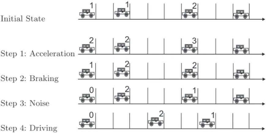
The model of Nagel and Schreckenberg belongs to the class of probabilis- tic cellular automaton models. N cars move along a one-dimensional lattice of length L (see Fig. 2.5). The state of each car is characterised by its po- sition xn ∈ {1, ..., L} and velocity vn ∈ {0, ..., vmax}. So obviously the state variables as well as the derived quantities like density ̺= NL or the distance dn=xn+1−xn−1 between two succeeding cars are discrete. Nearly all interac- tions are incorporated into determining the number of cellsvn(t+ 1) by which thenthcar is moved, during the next update step. Different rules are applied leading to a structure of substeps. As a parallel update is used, the rules are applied synchronously to all cars.
Step 1: Acceleration
Ifvn< vmax, increase velocity by one:
vn(t+14) = min{vn+ 1, vmax}
Step 2: Braking
Ifdn ≤vn, reduce velocity todn−1:
vn(t+24) = min{vn, dn−1}
Step 3: Noise
Ifvn>0, reduce velocity to vn−1 with probabilityp:
vn(t+34) = max{vn−1,0}with probabilityp
Step 4: Driving
Move car with velocityvn(t+ 1):
xn(t+ 1) =xn+vn(t+ 1)
The first step just increases velocity by one unit as long as the maximum velocityvmaxis not reached which is one of the models parameters. As this is the same for all cars, it corresponds to a speed limit rather than to the maximum of attainable speed which might be different for different vehicles. Overall this step reflects the wish of the drivers to move as fast as possible. The wish is of course restricted by the desire to avoid collisions. So in the second step, velocity is decreased such that collisions are avoided. For incorporating time latencies, only distancedn at timetis incorporated. It turns out, that this is already sufficient
for reproducing basic properties of real traffic flow [19]. The third step describes some randomness in the drivers’ behaviour by introducing a stochastic element namely the braking noise p. One reason is just that even on an uncrowded road where in principle driving is possible at an exactly constant speedvmax, small fluctuations are observed. But as density is low, the resulting effect will be small. The main effect of this step is the introduction of an asymmetry between acceleration and deceleration. Acceleration (if possible) takes place with probability 1−pwhereas deceleration occurs with probabilityp. This kind of asymmetry is also observed empirically (e.g. [34]). It originates just from the fact that braking leads to a stronger change in velocity than accelerating. So in the worst case a car brakes due to step 2 and slows down further due to step 3. The result might be the reduction of velocity by two units at one update whereas velocity can just increase by one unit per update. After applying the first three steps, velocity at timet+ 1 results in the movement of cars in step 4 byvn(t+ 1) sites.
Initial State
1 1 2
Step 1: Acceleration
2 2 3
Step 2: Braking
1 2 2
Step 3: Noise
0 2 1
Step 4: Driving
0 2 1
Fig. 2.5.Nagel-Schreckenberg model: The figures show the update procedure which basically consists of the application of the hopping rules to all cars at the same time.
For this particular example the maximum velocity was set to vmax = 3. In case of vmax = 1 the model turns out to be equivalent to the TASEP with time-parallel dynamics.
In comparison to theTASEP hopping now is allowed by more than one cell in a particular direction at one update. The number of cells for hopping is set according to the rules incorporating the drivers’ behaviour. As the cars ability to accelerate (and decelerate) is limited by inertia velocity can only increase by one unit per update. This induces some kind of memory to the process as the actual velocity depends on the velocity before the last update att−1. Also velocity itself is limited byvmax. With respect to reality a time-parallel update appears most realistic. It has been shown that some of the main features like
2.2 The TASEP 17
the occurrence of phantom jams [19, 65] depend on the use of that particular update procedure and also on the choice ofvmax>1.
For simulating real traffic flow parameters have to be chosen in accordance with the traffic system. A size of 7.5 meters for each cell is widely used. Although this is not the actual length of a normal car also larger vehicles like trucks are incorporated. Using that cell size leads to a density of one for (non-moving) vehicles forming a traffic jam. Typically vehicles are not waiting ”bumper to bumper” so the cell size also incorporates some kind of minimal distance.
As already mentioned velocity is limited to vmax for example by a speed limit. Also here a finer discretisation of velocity steps would be possible. For a German freeway the maximal velocity is frequently assumed to be 120kmh . So one identifies vmax = 5 with 120kmh . The randomisation parameter p is frequently set to p= 0.5. Overall the length of one timestep using the latter set of parameters is given by:
7.5m
cell ×[5−(0.5×1)]cell
time−step ×3.6sec
120m ≈1 sec
time−step (2.18) For calculating the time-scale the maximum velocity reduced by one unit through randomisation has been used. In comparison to reality the duration of one time-step is of the same order of magnitude as the typical reaction time of a driver. So this is in good agreement with the interpretation of the time-parallel update for incorporating time-latencies.
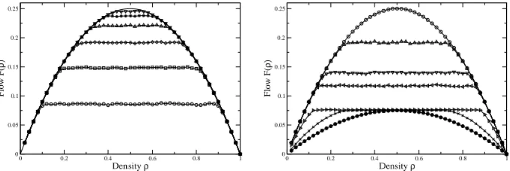
Simulation results from the Nagel-Schreckenberg model show some resem- blance to real traffic data [19]. The fundamental diagram forvmax= 5 exhibits features like the freeflow and the jammed state (see Fig. 2.7). At low densities flow shows a linear increase. Cars in principle can move at their desired velocity vmax. In the deterministic case of vanishing braking noisep= 0 no fluctuations in the drivers behaviour occur2. Due to the model’s rules cars will distribute homogeneously on the road (lattice). As long as the distance to the precededing car is large enough (dn≥vmax) cars are able to move constantly atvmax. The density at which cars begin to block each other therefore depends onvmax:
ρmax=N
L = N
N(vmax+ 1) = 1
vmax+ 1. (2.19)
Forρ > ρmaxthe average distance per car is given by ¯d=1ρ−1 = ¯v and is equal to the average velocity ¯v. Overall flow in both regimes is given by:
F(ρ) =
vmaxρ for ρ < ρmax
1−ρ else (2.20)
For 0< p <1 roughly the same behaviour is observed. One finds that due to fluctuations the transition to the jammed state occurs for ρ < ρmax. The corresponding spatial pattern of the jammed state is shown at (see Fig. 2.7).
2In case ofp= 1 a car is not able to increase velocity oncevn= 0 has been reached.
High density areas namely jams caused by fluctuations emerge and start trav- elling against the driving direction. But also due to fluctuations they dissolve again.
Fig. 2.6. Space-time plot and fundamental diagram: The space-time plot shows the lattice configuration for ρ= 0.2,p= 0.25 andvmax= 5. The fundamental diagram shows flow for different values ofvmax andp= 0.25. Forvmax= 1 the TASEP with time-parallel update is recovered (taken from [18]).
As shown above the distance between cars is a crucial quantity for char- acterising traffic states. So additionally distance headway distributions are of interest. In case ofvmax= 1 basically theTASEP is recovered (see Fig. 2.6). At low densities distances show a quite broad distribution. With increasing den- sity or equivalently decreasing available space the distribution gets less broad.
The probability fordn = 0 obviously corresponds to mutual blocking leading to vn= 0. So the probability fordn = 0 increases with increasing density. Us- ing analytical results originating from investigations of the TASEP with time- parallel update the probability fordnis exactly known (e.g. [19]). Fordn>0 one observes a monotonic decrease. For large velocities in case ofvmax= 5 roughly the same behaviour is found. A local maximum of probability at vmax = 5 reflects the fact that cars try to attaindn≤5.
Besides distance headways also time headways and single-car velocity dis- tributions are used for a microscopic characterisation of traffic flow [34, 50].
Each of the latter quantities has a corresponding macroscopic one [60]. Dis- tance headways correspond to density, time headways to flow and single-car velocities contribute to the average velocity. Some of them will be used for the investigations of ant-traffic in chapter 5.
2.3 The TASEP with Static Disorder
Another way of extending the TASEP for describing real systems is to incor- porate different kinds of quenched disorder. Two choices appear to be natural.
2.3 The TASEP with Static Disorder 19
Fig. 2.7. Distance headway distribution: For different values of ρ and vmax = 1(lef t),5(right) atp= 0.5 the distribution of distance headways has been measured.
On the left basically the distribution for theT ASEPcase is shown. For a larger range of attainable velocities maximums are shifted to higher densities (taken from [18]).
First one can introduce hopping rates depending on the particle i itself (par- ticlewise disorder). So one sets hopping rates according to p = pi which are independent of the particles’ position or time evolution. Complementary the second kind of disorder assigns hopping rates depending on the particles’ posi- tionxi(latticewise disorder). So hopping rates are set according top=p(xi). In this case the modified hopping rate of each particle is time independent in the sense that ponly depends on the positionxi itself. Generally all particles are affected in the same way. As a common feature of both types of disorder phase separation depending on the global particle density is observed. The emerging high- and low-density areas are in analogy to the shocks already known from plain TASEP with open boundaries. Basically the time evolution towards sta- tionarity as well as the stationary state itself are of interest. The formation of these high-density regions the so-called coarsening, during time evolution from a random initial distribution, has been studied in great detail [15, 38, 39, 53].
In the stationary state one is interested in the spatial distribution of particles depending on the global density.
Both kinds of disorder are encountered quite frequently. For example in vehicular traffic vehicles are generally not identical (e.g. different drivers, cars, trucks), leading to different driving characteristics. The resulting distribution of velocities can be used to assign different hopping rates. But also latticewise disorder is found quite frequently. Accidents or construction works, different local slopes of the road but also other inhomogeneities like different speed limits or on- and off-ramps might change the behaviour of the vehicles depending on the environment (e.g. [49]).
2.3.1 Particlewise Disorder
The TASEP with particlewise disorder has been studied in great detail. This was done for a random distribution of hopping rates [53,54]. Also a mapping to
thezero-range process [54, 78] and models of coalescence [27] has been shown.
Basically the formation of phase-separation as well as the dependence on the global density have been investigated. For a later comparison to the ant trail models a brief summary of the properties of the stationary state will be given.
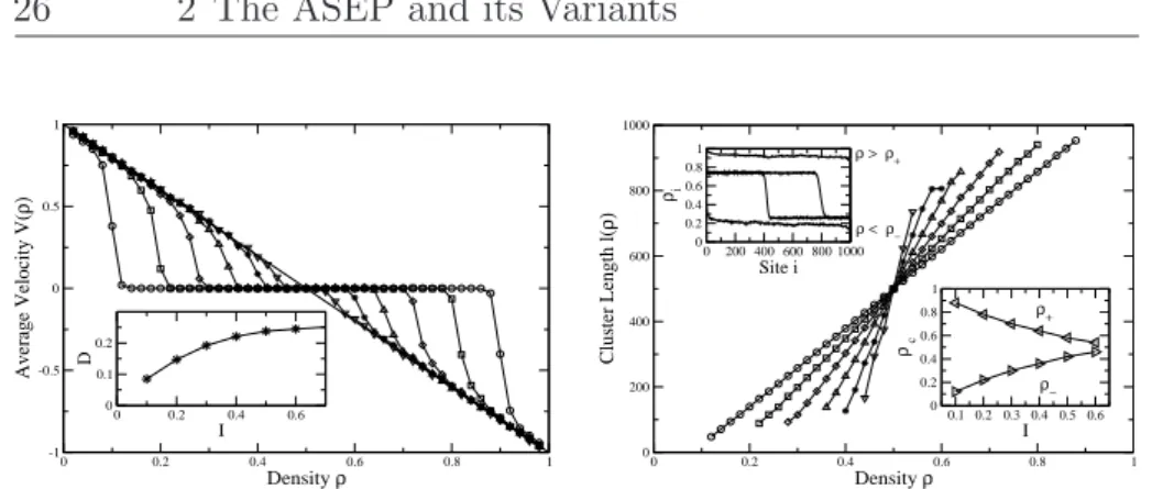
Generally the particles tend to move with an average velocity vi = pi if they are not blocked by another one. Due to the simple exclusion principle the ”faster” particles accumulate behind the slower ones which determine the average velocity of all other particles:
v= min
i∈[1,N]{pi} forρ < ρc. (2.21) In the stationary state a platoon moving with velocity v is formed (see Fig. 2.8). Like in the TASEP a characterisation using the density profile is possible. But the system is still translational invariant so phase-separations will not be localised. Therefore densities have to be measured relative to the moving system. Otherwise one just obtains a flat density profile as the platoon moves along the lattice with constant average velocity. By definition a second- class particle will follow the left end of the moving high-density area namely the platoon as this is just a domain-wall from ρ− = 0 to ρ+ >0. Measuring densities seen from that position will be used for characterising the structure of the particle distribution.
Fig. 2.8. Space-time plot: On the left the coarsening process out of a homogeneous distribution of particles in the initial state is shown. In the stationary state particles have accumulated behind the slowest one, forming a platoon. For that particular example only one ”slow” particle withp1= 0.1 and ” fast” particles withpi= 1∀i∈ {2, ..., N}have been used.
The densityhcii:=ρiat the site in front of theithparticle now defines the density profile. So densities are measured with respect to the moving particles.
Under the assumption that a mean-field description is still reasonable one finds
2.3 The TASEP with Static Disorder 21
(1−ρi)pi=v=const. ∀i∈[1, N] (2.22) as all particles within the platoon have to move with the same average velocity v. As long as the global density ρ is low enough this regime exists.
For a later comparison to the ant trail models it is sufficient to restrict to pi =: p > I ∀i ∈ {2, ..., N} and p1 := I = v. In case of ρ = 1− Ip = ρc
obviously no difference between the high- and low-density area can be made.
The first particle leading the platoon is also blocked with probability ρ like all the other particles. The two different regimes can be distinguished using second-class particles (see Fig. 2.9, right). In the jammed phase the second-class particle moves with the velocity of the platoon. As ρ− = 0 there is only drift and no diffusion. At high densities particles are distributed homogeneously.
The velocity of the second-class particle now depends on the global density according to (2.10).
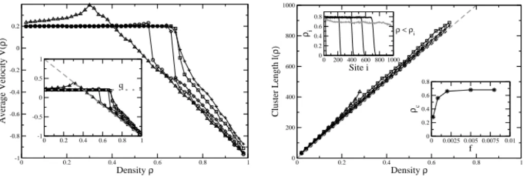
The density profile seen from the moving system can also be used for mea- suring the cluster length. By definition the cluster is the number of consecutive sites (particles) withρi> ρthus belonging to the high-density area:
l:= max
i∈[1,N]#
sites i |(ρi, ρi+1)> ρ= N L
(2.23) In the stationary state only one cluster exists comprising all particles of the system. Depending on the impurity hopping rateIa linear increase is observed (see Fig. 2.9, left). From (2.22) one also would have expected that kind of behaviour as the mean-field platoon length is given by:
ρi= 1− I pi
= N
l leading to l=L ρ 1−Ip
!
for pi=:p (2.24) From (2.24) one observes that the densityρi is independent of the particle numberN. So an increase of the global density is compensated by an increase of the cluster length and thus does not lead to an increase of ρi. The platoon length increases until the global densityρreaches the density within the moving platoonρi. As a result no difference between the densitiesρi andρ=NL can be made anymore asρi = 1−Ip =ρ. The cluster length reaches the system size.
Now also the leading particle becomes blocked and flow recovers the TASEP case. Nevertheless also the limitations of the mean-field picture become visible.
From (2.24) the cluster dissolves forl=L. But one observes that depending on Ithe cluster dissolves even forρ < ρc(see Fig. 2.9, left) beforel=Lis reached.
With increasing defect hopping rate obviously fluctuations also increase which are not incorporated by the mean-field approximation.
It has been pointed out that the transition from particles distributed homo- geneously on the latticeρ > ρc to the platoonρ < ρc exhibits some analogy to the Bose-Einstein condensation [54]. The unoccupied sites, namely the holes, are considered as bosons and the particles as states. For ρ > ρc most holes are distributed homogeneously. Each state is occupied with probability (1−ρ)
0 0.2 0.4 0.6 0.8 1
Density ρ
0 200 400 600 800 1000
Cluster Length l(ρ)
0 0.2 0.4 0.6 0.8 1
I
0 0.2 0.4 0.6 0.8 1
ρc
0 0.2 0.4 0.6 0.8 1
Density ρ
-1 -0.75 -0.5 -0.25 0 0.25 0.5 0.75 1
Average Velocity V(ρ)
Fig. 2.9.Cluster length and velocity of the second-class particle: (Q= 1,I= 0.1 (◦), 0.2(△), 0.3(▽), 0.4(⊳), 0.5(⊲), 0.6(×), 0.7(⋄), 0.8(∗), 0.9(•)). On the left the increase of the platoon length with increasing global densityρis shown. At a sufficiently high density ρc = 1−I (inset) the platoon vanishes. On the right the velocity of the second-class particle is shown. For ρ < ρc the particle performs drift following the platoon. Atρ > ρcthe TASEP is recovered.
at least for the TASEP with random-sequential dynamics. By reducing global density below ρc platoon formation takes place. Holes are distributed within the platoon with probability (1−ρi) = pIi. Depending on the platoon length the leading particle or equivalently the ground state has an occupation number of N1=L−l. In comparison to the others the leading particle has the largest num- ber of holes in front of it. Bosons obviously are condensed in the corresponding state. This has also been found in case of time-parallel update [27]. Never- theless this analogy is of a formal nature as bosons within an ideal Bose gas are non-interacting. They also condensate in real-space instead of momentum- space. But as particles in theTASEP are interacting this is also true for holes.
Even the choice of the update-procedure can induce interaction. A time-parallel update induces particle-hole attraction or equivalently hole-hole repulsion.
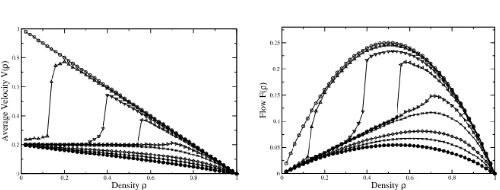
The stationary state is characterised using fundamental diagrams. Accord- ing to the already observed behaviour the average velocity stays constant for ρ∈[0, ρc(I)]. Flow shows a linear increase. For ρ∈[ρc(I),1] all particles have the same probability of being blocked. Obviously the TASEP case is recovered as mutual blocking dominates over different hopping rates.
2.3.2 Latticewise Disorder
Also the TASEP with quenched latticewise disorder has been studied in great detail [38, 39, 81, 82]. In comparison to particlewise disorder a larger number of variations has been introduced. With respect to a comparison to the features of the ant trail model we will focus here only on two of them. The most simple case is just one defect sitei0. Particles hopping fromi0toi0+ 1 have a reduced hopping rate I < p. At all other sites hopping takes place with rate p. With respect to reality also the case of extended defects p(xi) =I ∀i∈ {i1, ..., i2}
2.3 The TASEP with Static Disorder 23
0 0.2 0.4 0.6 0.8 1
Density ρ
0 0.2 0.4 0.6 0.8 1
Average Velocity V(ρ)
0 0.2 0.4 0.6 0.8 1
Density ρ
0 0.05 0.1 0.15 0.2 0.25
Flow F(ρ)
Fig. 2.10.Fundamental diagrams: (Q= 1,I= 0.1 (◦), 0.2(△), 0.3(▽), 0.4(⊳), 0.5(⊲), 0.6(×), 0.7(⋄), 0.8(∗), 0.9(•)). Forρ < ρcthe average velocity stays constant and flow increases linearly. At sufficiently high densities finally the TASEP case is recovered.
will be of interest. Other variants not being discussed here are for example a random distribution of defect sites [81, 82].
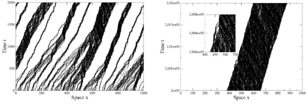
Starting from the spatial pattern exhibited by a system with one defect site one again observes a separation into a high- and low-density phase. Unlike in the case of particlewise disorder the areas are localised (see Fig. 2.11).
Fig. 2.11. Space-time plot: The left figure shows the formation of high- and low- density areas. On the right the stationary state has been reached. On the left of the defect sitexi0= 500 a high density area has formed.
As the density areas are static besides fluctuations at the boundaries [38,39]
this should also be visible in the second-class particles velocity (see Fig. 2.13, left). Depending on the global density one observes three regimes. Fluctuations obviously increase with increasing defect rateI(see Fig. 2.13, left, inset). Like in the case of particlewise disorder phase separation takes places starting at a density ρ− and ending atρ+(see Fig. 2.13, right, lower inset). One observes a particle-hole symmetry ρ− = 1−ρ+. This can also be seen in measuring
the length of the localised particle cluster namely the high-density regime. The cluster length obviously increases linearly with the global density (see Fig. 2.13, right). Investigating the density profile directly shows that this linear increase compensates additional particles originating from increasing the global density in such a way that the density in the high-density area stays constant (see Fig. 2.13, right, upper inset). This is possible until the cluster length reaches a critical value. Then an increase of the particle number can no longer be compensated. As a result the global density exceeds the density inside the high- density areaρ+ which obviously ceases to exist. In a similar way the existence of a lower bound ρ− for the regime can be explained. As long as the global density is belowρ− the system obviously is not able to segregate into a high- and a low-density area.
The fundamental diagrams also exhibit the three regimes already identified.
The average velocity shows a strict monotonic decrease. But flow exhibits a characteristic feature (see Fig. 2.12 left). Depending on the defect rate I flow becomes independent from density. The so-called plateau regime extends from ρ− to ρ+. For densities smaller than ρ− and larger than ρ+ the behaviour known from TASEP is recovered.
0 0.2 0.4 0.6 0.8 1
Density ρ
0 0.05 0.1 0.15 0.2 0.25
Flow F(ρ)
0 0.2 0.4 0.6 0.8 1
Density ρ
0 0.05 0.1 0.15 0.2 0.25
Flow F(ρ)
Fig. 2.12.Fundamental diagrams: On the left for one defect site withQ= 1,I= 0.1 (◦), 0.2(), 0.3(⋄), 0.4(△), 0.5(∗), 0.6(▽), 1 (solid line). The right figure shows flow for sitewise defects (Q= 1, I= 0.3) extending over lLd = 1(•), 0.5(×), 0.1(⊲), 0.0003 (⊳) 0.0001 (△) , 0 (◦). As a common features plateaus in flow exist.
Incorporating the described mechanisms a phenomenological approach has been developed for the case of random-sequential dynamics. Assuming a flat density profile within the macroscopic high- and low-density area flow is given by:
F−(ρ−) =ρ−(1−ρ−)p and F+(ρ+) =ρ+(1−ρ+)p (2.25) In accordance to the previous observations (see Fig. 2.13 right, upper inset) the particles can be assumed to be distributed homogeneously within the high-
2.3 The TASEP with Static Disorder 25
and low-density region. As the global density stays constant in time by defi- nition flow must be conserved due to the continuity equation:F− =F+. This leads to the already observed property of the density profile:ρ+= 1−ρ−.
Assuming that the region of decrease from ρ+ to ρ− at the defect site is negligible, the flow trough the defect is given by:
Fd(ρ−, ρ+) =ρ+(1−ρ−)I=ρ2+I= (1−ρ−)2I (2.26) As discussed the homogeneous distribution of particles namely the TASEP case is recovered forρ < ρ− and ρ > ρ+. The corresponding flow is then given by (2.25). For densities ρ− < ρ < ρ+ flow stays constant. Incorporating the flow through the defect site, the conservation of particles leads to:
ρ+= p
I+p and ρ− = I
I+p (2.27)
So overall the boundaries of the density regimes as well as the constant value of flow within the plateau regime (e.g. F = ρ+(I, p) [1−ρ+(I, p)]) are given by the two hopping ratesIand p.
Making use of the latter results the lengthl of the high-density regime can be calculated. For a total number ofN particles one finds:
N =lρ++ (L−l)ρ− leading to l(ρ) =L
ρ−ρ−
ρ+−ρ−
(2.28) Forρ < ρ−the cluster length becomes negative. It reaches the system length for ρ = ρ+. This is in analogy to a system with particlewise disorder where the leading particle becomes blocked as the platoon length reaches the system size. Overall the cluster-regime extends from l(ρ−) = 0 toρ+ =L. Again the mean-field picture fails to incorporate fluctuations (see Fig. 2.13 right). With increasing defect rate I the measured cluster length at the boundaries of the cluster-regime is above zero and below the system sizeL.
As an extension also multiple impurity-sites can be treated. One also finds the same basic properties like particle-hole symmetry as in the previously dis- cussed case (see Fig. 2.12 right). With increasing number of defect sites or defect-length in case of consecutive defects the plateau value decreases. A lower bound is given by the flow for a system with homogeneous hopping rate equiv- alent to the defect rate. Finally the plateau breaks down as approximately the TASEP case with hopping rateI is recovered.
Applying the same approach to multiple sites [81, 82] is also in good agree- ment with the simulations. As multiple shocks fromρ− toρ+exist the approx- imation is not as good as in the discussed case where only the increase for one shock has been neglected.