Scanning Tunneling Spectroscopy on Graphene Nanostructures

Scanning Tunneling Spectroscopy on Graphene Nanostructures

I n a u g u r a l - D i s s e r t a t i o n zur

Erlangung des Doktorgrades

der Mathematisch-Naturwissenschaftlichen Fakultät der Universität zu Köln

vorgelegt von

Diplom-Physiker Fabian Craes

aus Werl

Köln 2014

Erster Berichterstatter: Priv.-Doz. Dr. Carsten Busse Zweiter Berichterstatter: Prof. Dr. Achim Rosch

Vorsitz Prüfungskommission: Prof. Dr. Ladislav Bohatý

Tag der mündlichen Prüfung: 08.04.2014

Abstract

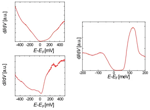
This thesis describes investigations on graphene nanostructures by the means of scanning tunneling microscopy (STM) and spectroscopy (STS) in ultra high vacuum at low temper- ature (5.5 K), focused on their electronic structure on the local scale. The experiments are based on structurally highly perfect epitaxial graphene on Ir(111) [gr/Ir(111)], but extend the range towards new graphene based nanomaterials.

The first topic comprises the development of new nanomaterials which keep the structural coherency of epitaxial graphene on Ir(111) at a reduced electronic substrate interaction, in particular concerning graphene’s quasi-relativistic Dirac particles. Therefor, we present the first study on graphene quantum dots (GQDs) on silver (gr/Ag). In STS, we observe the Ag(111) surface state on 15 ML of Ag on Ir(111), study its behavior in the presence of graphene, and discuss its role in the observation of Dirac electron confinement on GQDs.

We find the surface state suppressed in 1 ML of Ag on Ir(111).

In a next step we present an experimental advancement towards a system, where the metallic surface states are completely absent, namely oxygen covered Ir(111) [O/Ir(111)].

In an STS study, we discover new oxygen superstructures on iridium under graphene and two types of charge effects in the GQDs’ local density of states (LDOS). We present the first unambiguous experimental observation of Dirac electron confinement on GQDs [1]. We calculate the Dirac dispersion relation on the basis of our experimental data and confirm the efficient decoupling by DFT calculations and the direct observation of a Dirac feature in point spectroscopy and characteristic electron scattering processes. In addition to the benefit for the observation of Dirac confinement, our findings gain universal insight into the decoupling of graphene’s electronic system from the metallic substrate by oxygen intercalation.

The studies are extended towards the unoccupied surface state spectrum at high energies

in form of image potential states (IPSs). For the first time we experimentally prove the

size dependence of IPSs due to confinement on GQDs acting as a quantum well [2]. We

explain the occurrence of a strongly pronounced state, which is not the ground state, by

an interplay of the LDOS and momentum conservation during tunneling. The positions

of the IPSs can be tuned by chemical gating, which means the experimental realization

of a quantum well tunable in both width and depth. We discuss the benefit of a direct

measurement of the local workfunction for the determination of the local doping level in graphene intercalation compounds.

In a next step we propose a route how to experimentally access the binding situation at the boundaries of GQDs on Ir(111), using the advanced technique of Inelastic Electron Tunneling Spectroscopy (IETS).

Finally, we observe metallic features in the LDOS which are related to one dimensional

defects in an extended monolayer of epitaxial graphene on Ir(111).

Frequently used Symbols and Abbreviations

ARPES - Angle Resolved Photo-Emission Spectroscopy BZ - Brillouin zone

CVD - Chemical Vapor Deposition DFT - Density Functional Theory (L)DOS - (Local) Density of States fcc - face centered cubic

FWHM - Full Width at Half Maximum FT - Fourier Transformation GQD - Graphene Quantum Dot

gr - Graphene

IETS - Inelastic Electron Tunneling Spectroscopy

L - Langmuir, 1 L “ 1 ˆ 10

Torr ¨ s « 1 . 33 ˆ 10

mbar ¨ s LEED - Low-Energy Electron Diffraction [3]

LT-STM - Low Temperature Scanning Tunneling Microscope

ML - Monolayer

QMS - Quadrupole Mass Spectrometer

STS/STS - Scanning Tunneling Microscopy/Spectroscopy TPG - Temperature Programmed Growth

UHV - Ultra High Vacuum

XPS - X-Ray Photoemission Spectroscopy

XSW - X-Ray Standing Wave

Contents

I Introduction 1

1 Fundamentals 7

1.1 Scanning Tunneling Microscopy and Spectroscopy . . . . 8

1.2 Angle-Resolved Photoelectron Spectroscopy . . . 13

1.3 Freestanding Graphene . . . 14

1.4 Interacting Graphene . . . 16

1.5 Weakly Interacting Graphene . . . 19

1.6 Surface States . . . 22

1.7 Quantum Confinement of Electrons . . . 26

1.8 Electron Scattering Processes Observed by STM . . . 30

1.9 Imaging Graphene in STM . . . 33

2 Experimental Setup 37 2.1 Ultra High Vacuum . . . 39

2.2 Low Temperature . . . 40

2.3 Damping of External Excitations . . . 41

2.4 Scanning Tunneling Microscope . . . 41

3 Experimental Procedures 43 3.1 Sample Preparation . . . 44

3.2 Data Acquisition and Analysis . . . 49

II Results 51 4 Graphene Quantum Dots on Silver 53 4.1 Morphology . . . 54

4.2 The Ag(111) Surface State . . . 58

4.3 Dirac Feature of Graphene on Silver . . . 62

4.4 Confinement on Graphene Quantum Dots on Silver . . . 64

4.5 Suppressing the Silver Surface State . . . 68

4.6 Conclusion . . . 70

5 Charge Effects on Oxygen Intercalated Graphene Nanostructures on

Ir(111) 73

5.1 Morphology . . . 75

5.2 Observation of Charge Effects . . . 79

5.3 Conclusion . . . 92

6 Dirac Electron Confinement on Graphene Quantum Dots 93 6.1 Morphology . . . 97

6.2 Suppressing the Iridium Surface State . . . 99

6.3 Density Functional Theory . . . 102

6.4 Scanning Tunneling Spectroscopy . . . 103

6.5 Conclusion . . . 107

7 A Quantum Corral without a Fence 109 7.1 Size Dependent Shift of Image Potential States . . . 113

7.2 Preferred State in the Tunneling Process . . . 116

7.3 Mapping Confined Image Potential States . . . 118

7.4 Tuning the Depth of the Quantum Well . . . 122

7.5 Conclusion . . . 126

8 Inelastic Electron Tunneling Spectroscopy on Graphene Quantum Dots127 8.1 Probing the Edge . . . 128

8.2 Conclusion . . . 130

9 Metallic State at 1D Defects in Epitaxial Graphene on Ir(111) 133 9.1 Step Edge . . . 134

9.2 Structural Phase Boundary . . . 139

9.3 Conclusion . . . 140

10 Summary and Outlook 143 10.1 Summary . . . 144

10.2 Outlook . . . 146

III Appendix 147 A Details on Results 149 A.1 Fundamentals . . . 150

A.2 Dirac Electron Confinement on Graphene Quantum Dots . . . 153

A.3 A Quantum Corral Without a Fence . . . 153

B Technical Details on Scanning Tunneling Spectroscopy 155

B.1 Preparing a Spectroscopy Measurement . . . 156

B.2 Point Spectroscopy . . . 157

B.3 Constant Energy d I /d V Mapping . . . 160

B.4 Tip Forming with Vertical Manipulation . . . 162

B.5 d I /d V Energy Resolution . . . 162

B.6 Problems and Solutions . . . 163

C Acknowledgments 165

D Bibliography 169

IV Formal Addenda 195

E Deutsche Kurzzusammenfassung (German Abstract) 197 F Liste der Teilpublikationen (List of Publications) 199

G Offizielle Erklärung 201

PART I

Introduction

Layered and two dimensional materials provide access to exciting new physics as reduced dimensionality both offers a playground for testing important models in solid state physics and is of high relevance for technological applications. Two-dimensional materials differ significantly in their electronic, optical, mechanical and chemical properties from three dimensional bulk systems [4]. Very influential discoveries connected to reduced dimensionality include the quantum Hall effect [5], high temperature superconductivity [6, 7], topologically protected surface states [8], the Dirac electron systems of graphene [9, 10].

In recent years the two dimensional material graphene has become one of the most studied topics in solid state physics. Being the thinnest material in the world, graphene features a variety of stunning properties, ranging from outstanding structural to electronic properties, providing better electrical conductivity than silicon [11], better heat conductivity than copper [12], optical transparency [13, 14] and extreme mechanical robustness while being flexible at the same time [15].

The most striking properties of graphene are covered by its unique bandstructure, providing a usable energy range, where electrons move with a propagation speed independent of their energy, which is a behavior expected for massless particles [9, 16, 17]. Due to their mathematical description in a certain linear approximation, these charge carriers are called Dirac electrons [9]. For the first time revealing these striking features, in 2010 Andre Geim and Konstantin Novoselov were awarded the Nobel Prize in Physics “for groundbreaking experiments regarding the two-dimensional material graphene” [18]. Graphene evokes totally new physics, ranging from a high charge carrier mobility [19], easy doping [20], long spin coherence time [21] and the emergence of chiral edge states [22] to a half-integer quantum hall effect [16] and Klein-tunneling [23].

Two-dimensional materials are produced either directly by in-situ growth processes like the catalytic decomposition of a precursor on a substrate surface or molecular beam epitaxy, or by mechanical or chemical exfoliation from layered bulk crystals [24]. For the preparation of graphene all of these techniques have successfully been used. While actually the first detailed investigations have been performed on mechanically exfoliated layers of graphite [10, 24], an up-scalable process is predestined by liquid exfoliation [25, 26].

The preparation of graphene by in-situ growth processes on a substrate is obtained by

either thermally induced surface segregation from a carbon containing bulk substrate

like ruthenium or carbides (e.g. SiC) [27, 28] or by catalytic decomposition of organic

molecules on a metal surface [29]. These methods are successfully used for obtaining

samples with a high structural coherency [30, 31]. A further method of growing graphene

on metal surfaces is provided by ethylene cracking with an ion source and subsequent

thermally activated decomposition [32], directing the beam of ethylene fractions even to catalytically inactive noble metal surfaces [e.g. Cu(111), Au(111)]. With some of these methods graphene production can already reach the industrial scale with an implication for industrial applications [33, 34]. Potential applications for example include electromechanical devices [35], gas sensors [36, 37], photovoltaics [38], supercapacitors [39], and high frequency transistors [40].

Despite this promising perspective, there are of course obstacles in turning the new physics into applications. These are mainly based on the fact that on the one hand the in-situ growth of graphene on a substrate provides superior structural quality but on the other hand alters its electronic properties which are closely connected to a perfect energetic equivalence of all carbon atoms [41, 42]. Another fact is that in order to use graphene in semiconductor applications [43–45], it has to rest on an insulating substrate [30, 46]. However, playing the game of controlled graphene disturbance can also be a key to exciting new physics as well as applications on its own, since the presence of a tailored substrate enables the tuning of graphene with respect to its electronic and morphological structure, as well as its chemical properties [47–50]. Thus a tailored substrate aims either at quasi-freestanding graphene or tuned properties.

A very flexible way of obtaining such substrates is the intercalation of foreign species between epitaxial graphene and the supporting substrate. Here progress has been made concerning numerous different intercalants yielding a variety of new properties, including the species of oxygen [47, 51], silver [52], caesium [53], europium [49, 50], hydrogen [54], potassium [55], and bromine [56].

This work addresses the ambivalence of the substrate influence on graphene directly, playing with both structural and chemical degrees of freedom in highly tunable graphene systems. The regime of the 2 D material restricted even down to 1 D or 0 D extents reveals new physics, using the combination of scanning tunneling spectroscopy and electron confinement for addressing the electronic properties of the material in a nutshell:

We explore new graphene based nanomaterials with simultaneous structural coherency of

the carbon layer and maximum decoupling from the substrate, reporting on both silver

(Chap. 4) and oxygen intercalated graphene quantum dots (Chap. 5 and Chap. 6). Our

criterion for decoupling is the absence of covalent bonds to the substrate, still allowing

interaction in form of such an amount of charge transfer (doping) that the Fermi level still

resides in the energy range where the charge carriers are Dirac-like. We answer associated

questions referring to the critical parameters for observing Dirac electron features in these

systems and describe a route to suppress disturbing contributions of metallic surface

states to the local density of states. Several new aspects of the local electronic structure

of graphene quantum dots are discovered, namely inducing a shift of the silver surface

state (Chap. 4), new oxygen superstructures on Ir(111) (Chap. 5), charge effects (Chap. 5)

and the confinement of both Dirac (Chap. 6,[1]) and high energy free-electron surface

states (Chap. 7,[2]). Finally, we propose a way how to address the binding character at

the boundaries of graphene quantum dots (Chap. 8) and prove the existence of metallic

wires in one dimensional defects in extended graphene on Ir(111) (Chap. 9). Details on

the electronic structure of graphene, the most relevant aspects on surface electrons and

the envolved experimental techniques are provided in Chap. 1. The sample preparation

routines are discussed in very detail in Chap. 3 and a brief introduction to our experimental

setup appears in Chap. 2.

CHAPTER 1

Fundamentals

In this chapter a dense introduction to the most relevant aspects affecting

this work is given. Starting with the experimental techniques which have

been employed for this work we continue with an introduction into the field

of graphene. We provide an overview on the aspects of electronic behavior in

systems with reduced dimensionality, especially covering the topics of electron

scattering on surfaces and 2D confinement with a graphene bias. Finally, the

latter aspects are discussed from an STM point of view.

1 Fundamentals

1.1 Scanning Tunneling Microscopy and Spectroscopy

The topic of this section will be a brief introduction into the techniques of STM and STS as excellent tools for addressing alterations of the LDOS. Detailed descriptions of the STM principles are presented in Ref. [57].

Scanning Tunneling Microscopy

The scanning tunneling microscope (STM) has been developed in 1982 by G. Binnig and H.

Rohrer [58]. In 1986 they were awarded the Nobel Prize in Physics for this work. Based on the quantum mechanical tunneling effect, the microscope uses a very sharp - in the ideal case atomically sharp - conductive tip above a conductive sample surface in a distance of 5 .. 10 Å , forming two electrodes. In such a small distance the electronic wavefunctions of the closest atom of the tip and the sample overlap. Once applying a bias voltage V

between them, a tunneling current I sets in. The value of I depends on the LDOS of the tip and the sample, their distance z and the tunneling matrix element (i.e. the coupling of the initial and the final states). The exponential dependence of I on the distance z yields the extremely high vertical resolution of STM: A change in z of 1 Å results in a change in I of approximately one order of magnitude [59]. For imaging, the tip is moved along the surface, using piezo actuators. During this scanning process the distance z is controlled by a feedback loop circuit to a setpoint value of I (in constant current mode). Therefore, STM imaging is mainly determined by five parameters: The bias voltage V

, the tunneling current I and the spatial parameters z , x , y . According to Bardeen [60], I is given by

I 9 ż

´8

|M p E q |

ρ

p E ´ eV

q ρ

p E qr f p E ´ eV

q ´ f p E qsd E (1.1) with |M pE q| the tunneling matrix element, ρ

pE ´ eV

q and ρ

pEq the density of states of the tip and the sample at an applied bias voltage V

and fpEq the Fermi function.

A simple theory of STM is derived from (1.1) by Tersoff and Hamann [61], assuming a metallic s-orbital as the tip electrode and a bias voltage V

which is small compared to the workfunction of the sample Φ

( eV

ăă Φ

):

I 9 V

¨ ρ

p E

q ρ

p R

,E

q , (1.2)

with ρ

pR

,E

q the density of states of the sample surface at the center of the s-orbital

of the STM-tip R

. Since the DOS in first approximation decays exponentially into the

vacuum, one obtains an I depending inversely exponential on the distance z :

1.1 Scanning Tunneling Microscopy and Spectroscopy

Ipzq9e

. (1.3)

For the example of semiconductors eV

! Φ

does not hold anymore, therefore the description of I has to be modified. Especially deviating from the simple picture used above (Tersoff-Hamann), a finite energy range defined by V has to be taken into account by integration. A transmission probability (compare to Wentzel-Kramers Brillouin (WKB) approximation) T p V,W q is introduced, depending on V

and on the workfunction Φ

of the sample surface. With this one obtains I9

ż

EF

|T pV

, Φ

q|ρ

pEqρ

pR

,Eqd E. (1.4) The STM can be operated in different modes, depending on how the parameters V , I , and x,y,z are varied. For topographic imaging, all measurement in this work were performed using the constant current mode. This means keeping I and V

constant while varying the tip sample distance with a z feedback-loop in order to compensate for a varying sample LDOS while scanning the surface in the x and y directions. In this case the voltage which is used to elongate and shrink the z -piezo actuator for the distance variation on each surface coordinate ( x,y ) is recorded as the measurement quantity. Data recording is performed in an assignment of the modus operandi dependent measurement quantity to a matrix of N rows and M columns of discrete ( x,y ) surface coordinate tuples (STM image pixels).

Scanning Tunneling Spectroscopy

Scanning Tunneling Spectroscopy comprises all modes providing access to the LDOS of the surface. The most widely used modes are d I /d V ( E ´ E

) point spectroscopy and spatial constant energy mapping. Performing d I /d V ( E ´ E

) point spectroscopy requires fixing the tip-sample distance z at a certain coordinate ( x,y ) on the surface by choosing an appropriate setpoint of a bias voltage V

and a tunneling current I with closed feedback-loop and performing a subsequent onsite voltage sweep with open feedback-loop.

The latter means that the variation in the tunneling current as the measurement quantity

during the voltage sweep is not influenced by a varying orbital overlap of the tip and the

sample states by varying the tip-sample distance. Thus, the measurement signal is IpV q

depending on the sample LDOS at energies defined by eV “ E ´ E

. Decisive aspects are

the stability of the tip-surface distance (and also lateral position) regarding thermal drift,

the suppression of diffusion processes at the tip and the sample, and an improved energy

resolution (see below). Therefore, STS measurements are generally performed at low

1 Fundamentals

temperature (5.5K). According to Tersoff and Hamann the DOS at a surface coordinate is proportional to the differential conductivity d I /d V at fixed V

[61, 62]:

d I

d V 9|T |

ρ

pE

qρ

pE

q. (1.5) Since the transmission probability is difficult to access, |T | is often approximated by the total conductivity of the tunneling junction I {V [62]. The approximation works well for higher energies (several hundreds of meV to eV) and is problematical close to zero voltage since I p V “ 0q vanishes and thus I { V diverges.

Experimentally these values can be accessed by a direct measurement of

using the lock-in technique [61]. Therefor a weak AC voltage V

cosp ω tq is added to V

:

V “ V

` V

cospω tq.

The resulting tunneling current I is used as an input signal to a lock-in amplifier. This filters the ω AC fraction of the tunneling current via an integration of the product of I with a reference signal with the same frequency ω . As obtained by a Taylor expansion at V

in first order, the amplitude of the AC current fraction is proportional to d I /d V , and in second order proportional to the second derivative [63]:

IpV

` V

cospω tq “ IpV

` ∆ V q

» I p V

q ` dI p V q

dV p∆ V q ` d

I p V q dV

1

2 p∆ V q

` ...

» IpV

q ` dIpV q

dV pV

cospω tqq ` d

IpVq dV

1

2 pV

cospω tqq

` ...

» IpV

q ` dIpV q

dV pV

cospω tqq ` d

IpVq dV

1

4 V

p1 ` cosp2 ω tqq ` ...

The output signal of the lock-in amplifier can therefore be used for direct spectroscopic representation [64], either in d I /d V point spectra or in d I /d V spatial mapping at constant energy. In case of the latter one, a constant current topograph (integrated density of states) and a spatial map of the lock-in signal d I /d V at a fixed bias voltage V

are recorded simultaneously. One obtains a spatial distribution of the LDOS at an energy E “ E

` eV . STS provides the most local technique for spectroscopic investigations on a surface.

Difficulties include the facts that in reality the tip is not featureless in the sense of a free

electron gas as assumed in many calculations that due to vanishing tunneling transmission

probability it is impossible to measure sample states that do not overlap with states of the

tip and that it lacks chemical sensitivity. Controlling the microscopical shape of the tip

and thus the orbital which is involved in the tunneling process remains though, although

1.1 Scanning Tunneling Microscopy and Spectroscopy there are numerous efforts reported in literature for certain tip-sample combinations, e.g.

by adding molecules to the tip [65] or in spin-polarized STM [66].

The energy resolution depends on the temperature and the bias modulation used for the lock-in technique. According to [67] it amounts to:

∆ E “ ˘ 1 2

b

p3 . 3 k

T q

` p1 . 8 eV

q

.

Details of the lock-in preferences and parameters used for this work are described in Chap. B.

Inelastic Electron Tunneling Spectroscopy

As mentioned above, the second derivative is proportional to the second harmonic lock-in signal. Now I would like to draw a connection to the associated phenomenon of inelastic electron tunneling.

Inelastic Electron Tunneling Spectroscopy (IETS) in a simple picture is based on the fact that the charge transfer occurring with tunneling is able to cause a temporary charge redistribution in the object under investigation on the sample surface (e.g. a molecule) which is related to a change in molecular bond length. Since this redistribution might relax by exchanging charge with the substrate, a vibrational mode (phonon) is created and therefore directly connected to the tunneling current [68]. The tunneling process thus becomes inelastic via the relaxation process. Inelastic processes might also include the emission of light. The tunneling process mentioned is only possible if the connected phonon energy is allowed in the system. Thus, in the d I /d V spectrum this process will appear as a second tunneling channel in addition to the standard tunneling process generally assumed to be elastic. It shows a sudden step-like increase in the signal at a certain threshold energy (the phonon excitation energy ~ ν ) for both positive and negative bias voltages. The steps in d I /d V of course correspond to peaks in d

I /d V

, which is therefore a suitable quantity in IETS (see Fig. 1.1). Due to this mechanism, the most important criterion for identifying peaks in the second derivative of the I pV q characteristics as signatures of inelastic tunneling is their ˘~ ν mirror antisymmetry in energy with respect to 0 V ( E

):

Of course the direction of current does not induce any change to the excitation process.

The principles of charge redistribution and relaxation remain the same.

IETS is widely used to study molecular excitations on the local scale, requiring not more

than just one single molecule, making it the most sensitive technique for vibrational

excitation studies (e.g. [63, 69–71]). Another advantage is that, compared to infrared

(IR) and Raman spectroscopy [72], also optically forbidden excitations can be observed.

1 Fundamentals

Figure 1.1: (a) Schematic representation of elastic a and inelastic b tunneling processes between two electrodes (e.g. STM-tip and sample) at an applied bias voltage. (b) Conductivity IpV q (top) and its second derivative (bottom), indicating the features of the curves associated with elastic a and inelastic b tunneling processes. Reproduced from [69] with permission of The Royal Society of Chemistry.

Having its roots in metal/oxide/metal tunneling junctions (e.g. [73, 74]), it can be also realized in fixed-point STS as well as in STS spatial mapping [68, 75–78]. In the framework of this work it is therefore referred to as STM-IETS. This measurement technique has been extensively developed and used by the group of Wilson Ho [75, 79]. Via molecular excitations, STM-IETS provides chemical sensitivity in an indirect way which is lacking in elastic STM and STS.

In general STM-IETS requires the use of two lock-in amplifiers with a synchronized

reference signal, since this combination enables the simultaneous measurement of d I /d V

and d

I /d V

. In the framework of this thesis STM-IETS is applied for investigations on

the boundaries of GQDs presented in Chap. 8.

1.2 Angle-Resolved Photoelectron Spectroscopy

1.2 Angle-Resolved Photoelectron Spectroscopy

Angle-Resolved Photoelectron Spectroscopy (ARPES) is an experimental technique pri- marily aiming at the investigation of the occupied electronic structure in the reciprocal space of a solid’s surface and near-surface region. It also yields information on the lifetimes of excited states. ARPES is based on the photoelectric effect, measuring the kinetic energy of electrons emitted from the surface of an initial state with binding energy E

in the solid after absorption of a photon with energy ~ ν [59]. In the framework of this work photons were created with a helium discharge lamp (ultraviolet photoelectron spectroscopy). The kinetic energy of the photoelectrons leaving the surface is measured with an electron energy analyzer.

Often, the process is treated as a three-step process : The ‘optical excitation between the initial and final bulk Bloch eigenstates, travel of the excited electron to the surface, and escape of the photoelectron into vacuum after transmission through the surface potential barrier’ [80].

For the energy the process yields

E

“ ~ ν ´ Φ ´ E

(1.6)

with Φ the workfunction and E

the binding energy. If the translational symmetry of the sample surface is conserved, the in-plane component of the initial state momentum is also conserved:

~ k

“ ~ k

“ ~

a 2 mE

sin θ (1.7)

with θ the polar angle. Since the translational symmetry is not conserved in normal direction to the surface, k

is also not conserved. Details on ARPES are described in Refs. [80, 81].

The unoccupied spectrum can be probed using a more complex process called two-photon photoemission. Here, using a pulsed laser, a photon is used to excite an electron into an intermediate state in the unoccupied spectrum, a second one is used to probe the excited state in a photoemission process [82, 83].

In this thesis ARPES measurements are involved in the investigations on quantum con-

finement of Dirac electrons (see Chap. 6).

1 Fundamentals

1.3 Freestanding Graphene

Figure 1.2: Honeycomb lattice and its Brillouin zone. Top left: hon- eycomb lattice structure of graphene, made out of two interpenetrating triangular lattices (a

and a

are the lattice unit vectors, and δ

, i “ 1,2,3 are the nearest-neighbor vectors). Top right: corresponding first Brillouin zone in reciprocal space with unit vectors b

and b

, K and K

points.

The Dirac cones are located at the K and K

points. Bottom: energy spectrum in the units of the hopping parameter t as obtained from a tight binding calculation [9, 84]. Reprinted figures with permission from [9]. Copyright 2009 by the American Physical Society.

Freestanding graphene provides the basis for understanding the electronic structure in

absence of the complications induced by interactions with a substrate. The following

section gives a brief overview on the most important electronic properties of freestanding

graphene. For a more detailed introduction the reader is referred to literature, e.g. the

reviews of A. H. Castro Neto [9] and A. K. Geim [10].

1.3 Freestanding Graphene Graphene is formed by one monolayer of sp

hybridized carbon atoms in a honeycomb lattice, thus providing in total three sp

and one p

orbital at each of the two identical atoms in a unit cell. The structure can also be viewed as a superposition of two displaced triangular sublattices [9]. In the honeycomb lattice structure each atom is bound to three neighbors with a nearest-neighbor-distance of a

“1 . 42 Å

, resulting in three orbitals forming interconnecting σ bonds in-plane and leaving one p

-orbital out-of-plane. The neighboring, half-filled p

orbitals also overlap and form graphene’s π -system, giving rise to a delocalized electron system.

The unique electronic properties of graphene are intimately connected to the bandstructure at the K and K

points in the Brillouin Zone (BZ) (Dirac points, see Fig. 1.2) where the bonding and anti-bonding π bands touch at an energy E

“ E

with E

the Dirac energy and E

the Fermi energy (see Fig. 1.2). The band structure can be calculated with a tight-binding calculation [9, 26, 84], leading to

Epqq “ ˘t d

3 ` 2 cos ´ ? 3 k

a

¯

` 4 cos ˆ ?

3 2 k

a

˙ cos

ˆ 3 2 k

a

˙

with t the nearest neighbor hopping energy, the - sign for the occupied π -band, + for the unoccupied π *, a

the nearest neighbor distance, and q “ k ´ K the wavevector measured with respect to the K point.

At the Dirac points the bandstructure can be described in a linear approximation, using two-component wave functions and the 2 D relativistic Dirac-Weyl equation for massless quasiparticles [9, 10] with the Hamiltonian

H “ v

σq.

The two-component wave functions resemble properties of a spinor wavefunction and give rise to a pseudospin variable [9].

In this model, graphene’s electrons at the K points feature an energy-independent propa- gation speed with a (Fermi) velocity of v

“ 1 ˆ 10

m/s [85]. The character of graphene as a zero bandgap semiconductor is closely related to the perfect sublattice symmetry in freestanding graphene, with two identical C atoms in the unit cell. Unique properties like e.g. the anomalous integer quantum Hall effect [86], Klein tunneling [23] and 1D edge states [9] and Zitterbewegung [87] are related to the exceptional electronic features. Note that due to the low density of states in the vicinity of E

doping of graphene is highly effective and is achieved even by backgating [20].

1

the lattice constant results to a “1.42 ň ?

3=2.46 Å [84]

1 Fundamentals

A new class of Dirac electron systems is given by Topological Insulators (TIs). These 3(2)-dimensional bulk materials show 2(1)-dimensional surface states at their surface, which also behave like massless Dirac particles driven by a combination of strong spin-orbit coupling (SOC) and certain symmetries, e.g. connected to time reversal invariance (TRI) [8] or mirror symmetry [88, 89] of their bandstructure. Both classes of Dirac electron systems (graphene and TI) are distinguished by different topological invariants [ ν “ 0 (graphene), ν “ 1 (TI)] which experimentally e.g. lead to different quantization in the

fractional quantum hall effect [90].

Since it is the main issue of this section I would like to emphasize the importance of the sublattice symmetry of freestanding graphene. Since the two carbon atoms in the unit cell A and B are identical, ‘there are thus two zero-energy states: one in which the electron resides on atom A, the other in which the electron resides on atom B. Both the electron and hole states exist at exactly zero energy, hence zero band gap and zero mass’ [41]. This in turn means that massless dirac particles gain mass once the perfect sublattice symmetry is broken, the two C atoms in each unit cell are not at the same energy anymore [41]. Mass gain in graphene was recently shown for van der Waals heterostructures [42]. Sublattice asymmetry is basically also present for the systems discussed in the following sections together with hints how to restore it.

1.4 Interacting Graphene

Up to now large graphene areas can only be prepared by epitaxial growth on a substrate.

The best structural quality of graphene films is obtained by the decomposition of carbon

containing precursors on catalytically active metal surfaces, e.g. Pt(111) or Ir(111). The

presence of a substrate always influences the electronic properties of the graphene layer,

the deviation thus depends on the specific binding character to the substrate which in

general may vary spatially between a dominating physisorbed and chemisorbed character

[17, 26]. Due to a lattice mismatch with the respective substrate, epitaxial graphene shows

characteristic moiré superstructures as for example reported for the metal substrates

Ir(111) [91, 92], Cu(111) [93], Rh(111) [94], Pt(111) [95] and Ru(0001) [27]. The presence of

a substrate and the associated disturbance of graphene’s electronic system may be viewed

as a tradeoff for structural quality on a large scale. But it also opens new possibilities

of specifically tuning the electronic properties. Interesting comments on the pros and

cons of disturbing graphene are provided by Hasegawa et al. in Ref. [48] (references

adapted to the list of this work): ‘Electronic properties of this pristine nanostructure

1.4 Interacting Graphene

are easily modified by mechanical strains, deformations, metal contacts, adsorption of foreign atoms or molecules, external fields, and other physical contacts with environment.

These influences are unavoidable in most experiments as well as possible applications and easily impair intrinsic, novel properties of graphene. However, we can also make use of these effects to modulate electronic properties, thereby extending a range of technological applications. One of these examples is a bandgap opening, which is essential for graphene to be used for semiconductor devices. A substantial bandgap can be induced in several ways. Early examples are bandgap openings in epitaxial graphene on SiC (Refs.[96] and [97]) and graphene on hexagonal boron nitride (h-BN) [98]. A bandgap is also induced by electron confinement (nanoribbon) [99, 100], biasing [101, 102] or doping [103] bilayer graphene, patterning graphene with periodic holes (nanomesh or antidote lattice) [104, 105], or moiré-patterned hydrogen adsorption [106], and so on. These bandgap openings

can be interpreted in terms of either the hybridization of electronic states at K and K’

points in the Brillouin zone or the symmetry breaking of A and B sublattices by external or internal perturbations [96].’

This work uses gr/Ir(111) as a basis system for all experiments. Therefore, the next section provides an overview on the altering of graphene’s properties by the presence of the Ir(111) surface underneath.

Graphene on Ir(111)

The mismatch between the lattice constants of freestanding graphene a

“ 2 . 46 Å and Ir(111) a

“ 2 . 72 Å leads to a moiré superstructure with a lattice constant of a

“ 25 . 24 Å [17, 26]. The experimentally easily accessible moiré lattice constant together with the precisely known lattice constant of Ir(111) yields a lattice constant of gr/Ir(111) of a

“ 2 . 452p5q Å [17, 26]. Though providing superior structural quality and yielding a weak substrate interaction from the structural point of view [17], gr/Ir(111) shows significant signs of a substrate influence when it comes to the phononic and electronic properties. First, the typical Raman features of freestanding graphene are absent in gr/Ir(111) [107]. Second, altering of the electronic properties includes a band gap opening at the K point by about 70 meV [26], a doping of E

« 100 meV, the emergence of replica cones and minigaps caused by the moiré potential [108], the absence of defect states [109], the absence of characteristic p ?

3 ˆ ?

3qR 30

intervalley scattering patterns on extended

areas and the unclear observations of Dirac electron confinement on GQDs on Ir(111)

[110–113]. Further on, one of the two IPS series expected for freestanding graphene is

absent [114] (unlike e.g. in gr on SiC [115, 116]), indicating that the graphene surface

1 Fundamentals

Figure 1.3: DFT calculation of the moiré unit cell of gr/Ir(111). Top view (a) of the moiré unit cell with high symmetry regions (hcp, fcc, top) indicated by circles.

Side view (b) along the dashed line in (a) showing the first three layers of iridium atoms (white, red, and green spheres) and the carbon atoms (yellow) in same colour code as (a). Visualisation of the nonlocal-correlation binding-energy density (c) due to adsorption. Charge transfer (d) induced by adsorption, with magnification of the red box in (e). The range of the colour scale is -0.0138 Å

(blue) for a reduced electron density to +0.013 Å

(red) for an enhanced one, while green indicates the average electron density. Reprinted figure with permission from [17]. Copyright 2011 by the American Physical Society.

facing the substrate is definitely different from that one facing the vacuum side. Mostly this disturbance of graphene’s electronic structure can be viewed as a local instability of the predominating van der Waals bonding towards a more chemical character as mentioned above [17, 26], see Fig. 1.3.

In more detail, all the local electronic effects mentioned before face the fact that Ir(111) presumably provides two different types of surface states: First there is a typical Shockley- type surface state dispersing in the way of free electrons (parabolic dispersion) which was observed in several ARPES studies [92, 108, 114]. Second, there is a very local type of surface state, presumably originating from the localized, out-of-plane Ir(111) d

-orbitals, providing a flat dispersing surface state with high effective mass which hybridizes with graphene’s π -system [107]. The Shockley type surface state S

is known to be Rashba-split [1, 117]. It changes its properties when graphene is located on the surface [117]: The unperturbed Rashba-split band, evolving from E

“ ´0 . 34eV with negative effective mass, shifts upwards to E

“ ´0 . 19eV when graphene is on the surface.

Whereas the argument of missing intervalley scattering might be challenged by the fact that

the observation requires a certain value of defect concentration on the substrate providing a

sufficient amount of scatterers which is not present in gr/Ir(111) due to its high structural

1.5 Weakly Interacting Graphene quality, especially graphene’s behavior at defects [109] and edges of nanostructures like quantum dots [110] shows an even enhanced favored chemical binding of graphene to the substrate [118].

1.5 Weakly Interacting Graphene

Graphene Intercalation Compounds

One possible way of tuning the graphene-substrate interaction is the intercalation of species between the carbon layer and the substrate. Intercalation opens the window to a broad range of interesting topics as the presence of intercalants tunes the chemical character of the graphene sheet e.g. in the sense of adsorption sites for clusters [51] or ionic adsorbates [50] as well as the bonding character towards the substrate, depending on the specific intercalant with dramatic effects on the charge transfer occurring between graphene and the substrate. This immediately leads to the possibility of tuning the occupied density of states at E

by doping epitaxial graphene via intercalation [47]. Also structural changes in the graphene layer are closely connected to the changes in the binding character, e.g.

reduced moiré corrugation due to a reduced substrate interaction. One can even envision that intercalation processes can be used to tailor electronically structured graphene with neighboring regions of different doping levels [50] by using self-organized structures as observed in europium intercalation [49]. Aiming at freestanding graphene, by choosing an appropriate intercalant decoupling of the carbon layer in both a structural and an electronic sense is achievable. Intercalation can even be used for the exfoliation of an epitaxial graphene layer [56].

Oxygen Intercalated Graphene

Oxygen intercalation of gr/Ir(111) is achieved by exposing gr/Ir(111) to a dosage of molecular oxygen at an intercalation temperature where etching processes are absent [51].

The molecular oxygen dissociates on the uncovered Ir(111) surface. This necessary step

in the intercalation process limits the procedure to non closed graphene layers. Recent

publications comprising XPS and STM experiments report on the need for constant

oxygen pressure to make it favorable for the graphene edges to unbind from the substrate

[51]. This mechanism implies that the probability of a graphene area to be successfully

intercalated depends on the edge length. This leads to the fact that small islands with

short boundaries tend to resist intercalation. Vice versa the required temperature for

1 Fundamentals

successful intercalation also depends on the average size of the graphene structures. Results for small nanostructures, namely GQDs, are presented in Chap. 5. We show the first real space observations of the intercalation temperature influence on the oxygen superstructure realized underneath the GQDs. High temperatures (448 K) result in a dominating (2 ˆ 1) intercalation superstructure with respect to Ir(111). Those iridium areas which are not covered by graphene show the (2 ˆ 1) superstructure well known from the oxygen covered pristine iridium surface [51, 119]. Comparing pristine Ir covered by the (2 ˆ 1) oxygen superstructure with the situation of gr/O/Ir(111), XPS experiments report no difference in the Ir surface atoms binding energies [51]. In addition, no splitting of the C1s binding energies due to a hypothetical existence of C-O bonds is observed. In total, this indicates a situation where the oxygen is bound to the iridium. Especially the observed superstructures are expected to be with respect to Ir(111), yielding a weak interaction with the carbon layer. These findings are well supported by the results of XSW measurements on graphene intercalation compounds performed by Sven Runte [120], stating for oxygen intercalated graphene a closer distance of the oxygen atoms to the iridium substrate compared with the distance to the carbon layer. DFT calculations by Nicolae Atodiresei and Vasile Caciuc support the experimental findings by yielding the emergence of an oxygen-iridium hybrid state at the surface but absent binding between the oxygen and the carbon layers in contrast to the situation without an intercalant [1, 26]. Therefore oxygen is a decent intercalant to achieve decoupling of the carbon layer from the metal substrate. Oxygen intercalation alters the graphene bandstructure significantly by inducing a p-doping of about 600 meV [47].

Silver Intercalated Graphene

Like noble metals in general, also silver is expected to act as a weakly interacting substrate

for graphene. In theoretical studies graphene is expected to be physisorbed on the Ag(111)

surface and the Dirac cone is expected not to show a bandgap at all [48, 121]. Due to

the lack of catalytic activity, the method of choice for the growth of structurally highly

perfect graphene on metal substrates, the catalytic decomposition of ethylene, cannot be

used in this case. A possible way of obtaining graphene on silver is to use the standard

grown gr/Ir(111) and add a layer of silver by evaporation. Afterwards the sample is

heated, yielding an intercalation of the silver layer and resulting in the desired monolayer

graphene on silver configuration. The decoupling from the Ir(111) substrate can be tuned

by choosing the appropriate silver interlayer thickness. Silver intercalation of epitaxial

graphene is also proposed for the decoupling of graphene on Ni [48, 121]. An alternative

1.5 Weakly Interacting Graphene approach in preparation is presented in Ref. [122], using direct C evaporation from a graphite carbon source. This process also leads to gr/Ag which is experimentally found to be weakly interacting.

Like Ir(111) the Ag(111) surface shows a Shockley-type surface state. It has an onset energy of E

“ ´75 meV and is known to persist under 1 ML of several noble gases like Ar, Kr or Xe [123].

In a numerical study graphene on silver is discussed as a substrate in biosensor applications

[124].

1 Fundamentals

1.6 Surface States

After having reviewed some fundamental aspects of the 2D electron system of graphene, we turn to another 2D electron system, namely surface states of bulk solids. The presence of a surface has dramatic influence on the electronic states of a solid [59, 125, 126]. In contrast to the choice of periodic boundary conditions leading to Bloch waves with a real momentum k , the Schrödinger equation has to be solved with the boundary condition of a free surface. On the one hand the presence of a surface means an interface to the vacuum side, meaning a broken periodicity of the lattice potential in a 3D solid. On the other hand it also means an altering of the remaining periodic lattice potential close to the surface. This is especially valid for broken covalent bonds e.g. in semiconductors.

Connected to the high surface potential, all electronic wavefunctions have to decay exponentially into the vacuum. Since at the solid-vacuum interface the continuity of the wavefunction is postulated as a connection condition, also solutions of the Schrödinger equation which do not describe a meaningful physical behavior within the bulk region are recognized: Now also solutions with imaginary k momentum values become meaningful, which grow exponentially inside the bulk towards the surface but are now connected to the exponential decay at the interface, see Fig. 1.4. This situation corresponds to a locally enhanced probability density at the surface. In the framework of the nearly free electron approximation these states are referred to as (Shockley-)surface states, appearing predominantly in metals and small bandgap semiconductors. Surface states which are mathematically obtained by a pure tight-binding model with strongly perturbed surface potential (e.g. in d-electrons of transition metals, semiconductors, insulators) are referred to as Tamm-states [125]. Both types of surface states form two dimensional electron gases (parabolic dispersion) at the surface:

Epkq “ E

` ~

k

2 m

(1.8)

with m

the effective mass.

It can be shown that in the case of semiconductors and insulators these states are

energetically always located within the bandgap [126], in the case of metals in the projected

bulk band gap [59]. Therefore, at appropriate population surface states can basically act as

conducting states at the surface of bulk semiconductors or insulators, sometimes appearing

in rare combinations of physical properties like the spin-polarized surface state in the

ferromagnetic semiconductor EuO observed by our group [128]. However, their existence is

fragile with respect to the specific structure of the surface in the sense of local potentials.

1.6 Surface States

Figure 1.4: Solution of the Schrödinger equation for states localized at the surface:

The real part Ψ exponentially decays both into the bulk and the vacuum. The value z “ 0 determines the surface [127].

Adsorbates at the surface might cause a saturation of unsaturated bonds and therefore a bandgap in the surface state spectrum or even a vanishing of the surface states, killing a surface conductivity. Surface states which are degenerate with bulk states are called surface resonances. In sum, at the solid vacuum interface three types of electronic states in the occupied spectrum exist [57]:

• Bloch-bulk states which are delimited by the surface and therefore decay exponentially into the vacuum.

• Pure surface states, which decay exponentially into both the bulk and the vacuum and are located at the surface only.

• Surface resonances with a high amplitude at the surface and a reduced amplitude within the bulk as a Bloch-wave.

Image Potential States

In contrast to the occupied spectrum of surface states discussed before, image potential

states describe the unoccupied high energy spectrum of surface states, existing in an

attractive image charge Coulomb potential between the Fermi level E

and the vacuum

level E

` Φ (with Φ the local work function), as depicted in Fig.1.5. Perpendicular to

the surface they feature a hydrogen-like spectrum (characterized by a quantum number

n ) which converges to E

` Φ [130], parallel to it a two dimensional electron gas (2DEG)

forms with a continuous distribution of parallel momentum k for the case of extended

systems. States Ψ

pkq with energies E

pkq result. In STM, IPSs appear as peaks in

the local density of states (LDOS) measured while retracting the tip from the surface.

1 Fundamentals

Figure 1.5: Schematic depiction of the n “ 1 and n “ 2 IPS wavefunctions, energetically residing in the projected bulk band gap. With increasing n, the weight of the wavefunction moves further away from the surface (see z scale). Reprinted from [129].

As they are Stark-shifted due to the electric field between the tip and the sample [131]

they are often referred to as field emission resonances. Fig.1.6 depicts the influence of the

z z z

f

f

f

f

f

f

V V V

sample sample

sample tip

tip tip

Figure 1.6: Compensating the Stark shift within one voltage sweep in constant current mode: Comparison of the effective tunneling barrier for different bias voltage and tip-sample distance. See text for detailed discussion.

constant current mode on measuring IPS in d I /d V point spectroscopy: From left to right

the sketch depicts the potentials of the tip and the sample (gray boxes) which are spatially

separated by a distance z . Adding the workfunctions of the tip and the sample Φ

and

Φ

, one obtains the triangular tunneling barrier which area can be controlled by the bias

voltage (potential difference). The effective tunneling barrier is colored dark blue, the area

is relevant for the tunneling probability. For the case of IPS, a Coulomb potential is added

(dashed line). The IPS spectrum is sketched by red lines in the Coulomb potential. In the

1.6 Surface States center image, the same situation is plotted for the case of an increased bias voltage (in this example by lowering the sample potential). The area of the effective tunneling barrier is reduced, increasing the tunneling probability and thus the tunneling current. At the same time the potential for the IPS is broadened, changing the IPS spectrum by reducing the energetic distance of neighboring states. In constant current mode the distance z is consequently increased in order to restore the initial area of the effective tunneling barrier (right picture). This is accompanied with restoring the initial width of the potential for the IPS, restoring the initial spectrum in the sense of energy splitting. The absolute positions in energy are not conserved. This process is important in the continuous increase of V

in a constant current point spectroscopy voltage ramp with active feedback as it is used in Chap. 7.

Surface states play an important role in the framework of this thesis as they compete

with Dirac electrons in the LDOS of epitaxial graphene systems and therefor affect our

investigations on quantum confinement on GQDs (see Chap. 4 and Chap. 6). Image

potential states on GQDs are investigated in Chap. 7.

1 Fundamentals

1.7 Quantum Confinement of Electrons

Quantum confinement of electrons describes the altering of a materials electronic system by reduced dimensionality in the order of the electronic wavelength. The most prominent experimental example is the real space imaging of the electrons of a 2D electron gas confined to a ring of iron atoms on Cu(111), imaged by scanning tunneling microscopy [132, 133]. Intensive investigations of the outstanding electronic and optical properties of 0D structures have been performed in the field of semiconductor quantum dots [134].

Low dimensional electron systems are supposed to have potential application in quantum computing [135] and opto-electrical applications (e.g. solar cells [136–138]) while being already available in upscalable processes [139].

Figure 1.7: Electron confinement pattern as observed on an oxygen intercalated GQD on Ir(111) by STS. Compare (1,1) in Fig. 1.8.

In most cases reduced spatial dimensionality is connected to a rise of the potential energy

at the boundary of a nanostructure, creating a local minimum inside which in this case

is commonly referred to as a quantum well. A direct consequence is the localization of

initially free electrons of a metallic band in a standing wave pattern risen by the scattering

of electronic waves on the opposing walls of the quantum well and subsequent quantum

mechanical interference as it is well known from the particle-in-a-box problem [140]. The

example of a cylindrical potential well is presented as an excerpt of the master thesis of

1.7 Quantum Confinement of Electrons Wouter Jolie [141] in Chap. A, a plot of the six lowest energy Bessel eigenstates in this geometry is presented in Fig. 1.8.

The confinement is accompanied by a lift of the states of a metallic band, giving rise to discrete atom-like states (characterized by a set of quantum numbers). This is due to the fact that at least for an infinite potential outside the well the wavefunction has to vanish at the boundary, implying that only discrete values for the momentum k are allowed. Therefore, the discretization in energy and momentum is a clear quantum size effect, providing two main parameters for tuning the confinement character of a quantum well, namely its width and the strength of the potential at its boundaries. Whereby the latter one is tuned by doping [142].

A quantitative description of electron confinement is given by mainly two different models:

At first the perturbation of the density of states by screening the presence of the potential well, which is referred to as the Friedel oscillation picture [143]. Second the more qualitative, but more simple single electron model, assuming a single electron wave being backscattered from a hard wall potential well and subsequent interference [132]. The latter model can be modified by adding the possibility of inelastic scattering (soft wall), leading to a more quantitative description [144].

(1,0) (1,1) (2,0)

(2,1) (2,2) (3,0)

Figure 1.8: The first six confined states (Bessel eigenstates) (m,l ) for an infinite cylindrical potential well. Compare Fig. 1.7, Fig. 4.8, Fig. 6.8, and Fig. 7.5.

For the case of graphene, ‘confinement can be produced either by etching, by the reduced

dimensions of the graphene crystallites or by the application of gate potentials (here Klein

tunneling poses strong limitations on the use of such a method)’ [145]. For confining Dirac

electrons on extended graphene, the use of inhomogeneous magnetic fields is proposed

1 Fundamentals

[146]. The experimental observation of quantum confinement on nanopatterned graphene was first reported in Ref. [147].

Confinement on GQDs on Ir(111) is described in Refs. [110–113]. However, aiming at a proof for the observation of a confinement of graphene’s linear dispersing Dirac electrons, these publications were challenged by [112], stating that the observations were mainly due to a confinement of Ir(111) surface states below the GQDs. In Chap. 6 we show that the problem of unclear assignment of the observed confinement structures on epitaxial GQDs is fixed by suppressing these surface states [1]. In Chap. 7 we demonstrate the first observation of confined high energy surface states in a tunable quantum well [2].

Though there are hints that confinement of Dirac particles differs from the one of Schroedinger electrons [148, 149], our system can be approached by a simple model [110, 111, 113]: For an analytical treatment and the determination of the wave vector k belonging to a state with specific E we approximate a GQD with an area A as an infinite cylindrical well with radius r “ a

A { π [150]. In this case, the eigenstates in polar coordinates pρ,φq are given by

Ψ

9J

pk

ρqe

, (1.9)

where J

is the spherical Bessel function of the first kind with order l [132]. Details on the Bessel functions are provided in A.3. The continuous distribution of k breaks down into discrete values k

. Due to the confinement, Ψ

must have a node for ρ “ r , leading to the condition

k

r “ z

(1.10)

with z

the m -th zero of J

, i.e., the eigenstates can be characterized by quantum numbers m and l , hence Ψ

or pm,lq in shortened notation. The momentum k

of a given state pm,lq observed at an energy E can thus be calculated via

k

“ z

{r “ z

a

π{A. (1.11)

The energies of the eigenstates are given by

E

“ E

` p ~

π{2q ¨ z

{pA ¨ m

q, (1.12) with E

the energy of the state on extended graphene and m

the effective electron mass.

For r Ñ 8, this equation converges to the dispersion relation of free electrons, see Sec. A.1.

1.7 Quantum Confinement of Electrons Due to the long spin coherence time in graphene, a discussion of a potential use of GQDs in quantum computing was started by Trauzettel et al. [21]. Recently it has been shown that also plasmons can be confined in graphene nanostructures [151, 152].

Quantum confinement is the basic concept for most of the results presented in this thesis,

see Chap. 4, Chap. 5, Chap. 6 and Chap. 7.

1 Fundamentals

1.8 Electron Scattering Processes Observed by STM

In everyday life we are surrounded by many macroscopic examples of particle scattering, like light scattering at dust particles or photons scattering at the edge of a slit, showing diffraction and interference effects. In normal direction to a scatterer the translational symmetry is broken while it is conserved in the parallel direction. Here, scattering processes are closely related to Noether’s theorem. It implies that the momentum is only conserved in the parallel direction (e.g. to a slit) while it is not conserved in the normal direction, requiring a momentum transfer.

Thinking about scattering of electrons at atomic size point defects or nanostructures like a surface step, of course quantum mechanics in solid state systems comes into play. The setting should be described by scatterers as perturbations of the density of states (DOS), since the DOS involves all necessary concepts for a realistic picture of the material’s electronic structure. Therefore the picture of a single electron wave scattering at a defect and forming a standing wave by interfering with a reflected version of itself is often an oversimplified one. It does not take into account the presence of the bulk electrons, nor that there is a pronounced difference between LDOS and d I /d V in the vicinity of perturbations:

This issue becomes of vital importance when deriving a surface state dispersion from STS measurements, like in the pioneering work of Crommie et al. on Cu and of Hasegawa and Avouris on Au [153, 154]. Here a significant deviation from the dispersion relations measured by PES showed up, due to the oscillations in the total density of states connected to a screening of the impurity, which are commonly referred to as Friedel oscillations [143]. In STS data analysis these Friedel oscillations are considered by either adding an oscillating surface potential term [153] or considering an oscillating background in the d I /d V signal like in the detailed description by Hörmandinger [155].

In terms of scattering observations, d I /d V is found to reproduce the LDOS oscillations best in constant height mode and far away from a scattering site [155]. This means some contradiction to the experimental reality since at least the latter collides with the fact that the oscillations experience a quite strong damping (e.g. by electron phonon coupling).

The Friedel contribution becomes more severe the larger the energy range E ´ E

gets,

but is still present in spectroscopic constant energy mapping since the Lock-in technique

also involves the energy range provided by voltage modulation. In the latter case and in

case of using very low voltage (few mV) STM topographs, the observed oscillations are

sometimes referred to as energy resolved Friedel oscillations, e.g. in Ref. [156].