Parallel Computing
Peter Bastian
email: peter.bastian@iwr.uni-heidelberg.de Olaf Ippisch
email: olaf.ippisch@iwr.uni-heidelberg.de November 9, 2009
Contents
1 Parallel Computing 3
1.1 Introduction . . . 3
1.1.1 Why Parallel Computing ? . . . 3
1.1.2 (Very Short) History of Supercomputers . . . 4
1.2 Single Processor Architecture . . . 6
1.2.1 Von Neumann Architecture . . . 6
1.2.2 Pipelining . . . 7
1.2.3 Superscalar Architecture . . . 8
1.2.4 Caches . . . 9
1.3 Parallel Architectures . . . 12
1.3.1 Classifications . . . 12
1.3.2 Uniform Memory Access Architecture . . . 13
1.3.3 Nonuniform Memory Access Architecture . . . 14
1.3.4 Private Memory Architecture . . . 17
1.4 Things to Remember . . . 19
2 Parallel Programming 20 2.1 A Simple Notation for Parallel Programs . . . 20
2.2 First Parallel Programm . . . 20
2.3 Mutual Exclusion . . . 22
2.4 Single Program Multiple Data . . . 23
2.5 Condition Synchronisation . . . 24
2.6 Barriers . . . 25
2.6.1 Things to Remember . . . 26
3 OpenMP 27 4 Basics of Parallel Algorithms 32 4.1 Data Decomposition . . . 33
4.2 Agglomeration . . . 35
4.3 Mapping of Processes to Processors . . . 36
4.4 Load Balancing . . . 36
4.5 Data Decomposition of Vectors and Matrices . . . 37
4.6 Matrix-Vector Multiplication . . . 40
4.6.1 Things to Remember . . . 41
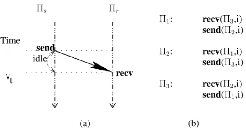
5 Introduction Message Passing 41 5.1 Synchronous Communication . . . 43
5.2 Asynchronous Communication . . . 45
6 Debugging of Parallel Programs 45 7 The Message Passing Interface 47 7.1 Simple Example . . . 47
7.2 Communicators and Topologies . . . 50
7.3 Blocking Communication . . . 51
7.4 Non-blocking communication . . . 53
7.5 Global Communication . . . 54
7.6 Avoiding Deadlocks: Coloring . . . 55
8 Things to Remember 57 9 Analysis of Parallel Algorithms 58 9.1 Examples . . . 60
9.1.1 Scalar Product . . . 60
9.1.2 Gaussian Elimination . . . 61
9.1.3 Grid Algorithm . . . 62
9.2 Scalability . . . 64
9.2.1 Fixed Size . . . 64
9.2.2 Scaled Size . . . 65
9.3 Things to Remember . . . 67
10 Programming with CUDA 67 10.1 Introduction . . . 67
10.2 Hardware Implementation . . . 70
10.3 CUDA examples . . . 72
1 Parallel Computing 1.1 Introduction
This set of lectures gives a basic introduction to the subject.
At the end you should have acquired:
• A basic understanding of different parallel computer architectures.
• Know how to write programs using OpenMP.
• Know how to write programs using message passing.
• Know how to write parallel programs using the CUDA environment.
• Know how to evaluate the quality of a parallel algorithm and its implementation.
1.1.1 Why Parallel Computing ? Parallel Computing is Ubiquitous
• Multi-Tasking
– Several independent computations (“threads of control”) can be run quasi-simultaneously on a single processor (time slicing).
– Developed since 1960s to increase throughput.
– Interactive applications require “to do many things in parallel”.
– All relevant coordination problems are already present (That is why we can “simu- late” parallel programming on a single PC”.
– “Hyperthreading” does the simulation in hardware.
– Most processors today offer execution in parallel (“multi-core”).
• Distributed Computing
– Computation is inherently distributed because the information is distributed.
– Example: Running a world-wide company or a bank.
– Issues are: Communication across platforms, portability and security.
• High-Performance Computing
– HPC is the driving force behind the development of computers.
– All techniques implemented in today’s desktop machines have been developed in supercomputers many years ago.
– Applications run on supercomputers are mostly numerical simulations.
– Grand Challenges: Cosmology, protein folding, prediction of earth-quakes, climate and ocean flows, . . .
– but also: nuclear weapon simulation
– ASCI (Advanced Simulation and Computing) Program funding: $ 300 million in 2004.
– Earth simulator (largest computer in the world from 2002 to 2004) cost about$500 million.
1.1.2 (Very Short) History of Supercomputers What is a Supercomputer?
• A computer that costs more than$10 million
Computer Year $ MHz MBytes MFLOP/s
CDC 6600 1964 7M$ 10 0.5 3.3
Cray 1A 1976 8M$ 80 8 20
Cray X-MP/48 1986 15M$ 118 64 220
C90 1996 250 2048 5000
ASCI Red 1997 220 1.2·106 2.4·106
Pentium 4 2002 1500 2400 1000 4800
Intel QX 9770 2008 1200 3200 >4000 106
• Speed is measured in floating point operations per second (FLOP/s).
• Current supercomputers are large collections of microprocessors
• Today’s desktop PC is yesterdays supercomputer.
• www.top500.orgcompiles list of supercomputers every six months.
Development of Microprocessors
Microprocessors outperform conventional supercomputers in the mid 90s (from Culler et al.).
Development of Multiprocessors
Massively parallel machines outperform vector parallel machines in the early 90s (fromCuller et al.).
TOP 500 November 2007
3. BlueGene/P “JUGENE” at FZ J¨ulich: 294912 processors(cores), 825.5 TFLOP/s
Terascale Simulation Facility
BlueGene/L prototype at Lawrence Livermore National Laboratory outperforms Earth Simu- lator in late 2004: 65536 processors, 136 TFLOP/s,
Final version at LLNL in 2006: 212992 processors, 478 TFLOP/s Efficient Algorithms are Important!
• Computation time for solving (certain) systems of linear equations on a computer with 1 GFLOP/s.
N Gauss (23N3) Multigrid (100N) 1.000 0.66 s 10−4 s 10.000 660 s 10−3 s
100.000 7.6 d 10−2 s
1·106 21 y 0.1 s
1·107 21.000 y 1 s
• Parallelisation does not help an inefficient algorithm.
• We must parallelise algorithms with good sequential complexity.
1.2 Single Processor Architecture 1.2.1 Von Neumann Architecture Von Neumann Computer
instructions
Memory CPU
controls
IU
PC Registers
ALU
data
IU: Instruction unit PC: Program counter ALU: Arithmetic logic unit CPU: Central processing unit Single cycle architecture 1.2.2 Pipelining
Pipelining: General Principle
....
....
....
.... ....
τ 2τ 3τ 4τ
x1
x1
x1
x1
x2
x2
x2
x2
x3
x3
x3
x3 x4
x4
x4
T1
T2
T3
T4
time
• TaskT can be subdivided intom subtasksT1, . . . , Tm.
• Every subtask can be processed in thesame timeτ.
• All subtasks areindependent.
• Time for processingN tasks:
TS(N) =Nmτ TP(N) = (m+N−1)τ.
• Speedup S(N) = TTS(N)
P(N) =mm+NN−1. Arithmetic Pipelining
• Apply pipelining principle to floating point operations.
• Especially suited for “vector operations” likes=x·yorx=y+zbecause of independence property.
• Hence the name “vector processor”.
• Allows at mostm= 10. . .20.
• Vector processors typically have a very high memory bandwith.
• This is achieved with interleaved memory, which is pipelining applied to the memory subsystem.
Instruction Pipelining
• Apply pipelining principle to the processing of machine instructions.
• Aim: Process one instruction per cycle.
• Typical subtasks are (m=5):
– Instruction fetch.
– Instruction decode.
– Instruction execute.
– Memory access.
– Write back results to register file.
• Reduced instruction set computer (RISC): Use simple and homogeneous set of instruc- tions to enable pipelining (e. g. load/store architecture).
• Conditional jumps pose problems and require some effort such as branch prediction units.
• Optimising compilers are also essential (instruction reordering, loop unrolling, etc.).
1.2.3 Superscalar Architecture Superscalar Architecture
• Consider the statements (1) a = b+c;
(2) d = e*f;
(3) g = a-d;
(4) h = i*j;
• Statements 1, 2 and 4 can be executed in parallel because they are independent.
• This requires
– Ability to issue several instructions in one cycle.
– Multiple functional units.
– Out of order execution.
– Speculative execution.
• A processor executing more than one instruction per cycle is called superscalar.
• Multiple issue is possible through:
– A wide memory access reading two instructions.
– Very long instruction words.
• Multiple functional units with out of order execution were implemented in the CDC 6600 in 1964.
• A degree of parallelism of 3. . . 5 can be achieved.
1.2.4 Caches Caches I
While the processing power increases with parallisation, the memory bandwidth usually does not
• Reading a 64-bit word from DRAM memory can cost up to 50 cycles.
• Building fast memory is possible but too expensive per bit for large memories.
• Hierarchical cache: Check if data is in the levell cache, if not ask the next higher level.
• Repeat until main memory is asked.
• Data is transferred incache lines of 32 . . . 128 bytes (4 to 16 words).
0000 0000 1111 1111
00 00 0 11 11 1 0000 0000 0000 1111 1111 1111
greater slower
Processor Registers
Level 1 cache
Level 2 cache
Main memory
Caches II
• Caches rely onspatial and temporal locality.
• There are four issues to be discussed in cache design:
– Placement: Where does a block from main memory go in the cache? Direct mapped cache, associative cache.
– Identification: How to find out if a block is already in cache?
– Replacement: Which block is removed from a full cache?
– Write strategy: How is write access handled? Write-through and write-back caches.
• Caches require to make code cache-aware. This is usually non-trivial and not done automatically.
• Caches can lead to a slow-down if data is accessed randomly and not reused.
Cache Use in Matrix Multiplication
• Compute product of two matricesC=AB, i.e. Cij =PN
k=1AikBkj
• Assume cache lines containing four numbers. C layout:
A B
A0,0
A15,0
A0,15
Matrix Multiplication Performance
BLAS1 Performance
Laplace Performance
1.3 Parallel Architectures 1.3.1 Classifications
Flynn’s Classification (1972)
Single data stream Multiple data streams (One ALU) (Several ALUs)
Single instruction SISD SIMD
stream, (One IU)
Multiple instruction — MIMD
streams (Several IUs)
• SIMDmachines allow the synchronous execution of one instruction on multiple ALUs.
Important machines: ILLIAC IV, CM-2, MasPar. And now CUDA!
• MIMD is the leading concept since the early 90s. All current supercomputers are of this type.
Classification by Memory Access
• Flynn’s classification does not statehow the individual components exchange data.
• There are only two basic concepts.
• Communication via shared memory. This means that all processors share aglobal address space. These machines are also calledmultiprocessors.
• Communication via message exchange. In this model every processor has its own local address space. These machines are also calledmulticomputers.
1.3.2 Uniform Memory Access Architecture Uniform Memory Access Architecture
P P
P
C C
C
Connection network
Memory
• UMA: Access to every memory location from every processor takes the same amount of time.
• This is achieved through adynamic network.
• Simplest “network”: bus.
• Caches serve two reasons: Provide fast memory access (migration) and remove traffic from network (replication).
• Cache coherence problem: Suppose one memory block is in two or more caches and is written by a processor. What to do now?
Bus Snooping, MESI-Protocol
remote read miss
hit read read hit
remote read miss
I
M S
E
read miss invalidate write hit
read miss
invalidate write hit hit
read/write
write miss invalidate (write back)
remote read miss (write back)
• Assume that network is a bus.
• All cacheslisten on the bus whether one of their blocks is affected.
• MESI-Protocol: Every block in a cache is in one of four states: Modified, exclusive, shared, invalid.
• Write-invalidate, write-back protocol.
• State transition diagram is given on the left.
• Used e.g. in the Pentium.
1.3.3 Nonuniform Memory Access Architecture Nonuniform Memory Access Architecture
P
P C C
Connection network
Memory Memory
• Memories are associated with processors but address space is global.
• Access to local memory is fast.
• Access to remote memories is via the network and slow.
• Including caches there are at least three different access times.
• Solving the cache-coherence problem requires expensive hardware (ccNUMA).
• Machines up to 1024 processors have been built.
AMD Hammer Architecture Generation 8, introduced 2001
Barcelona QuadCore, Generation 10h, 2007
Barcelona Core
Barcelona Details
• L1 Cache
– 64K instructions, 64K data.
– Cache line 64 Bytes.
– 2 way associative, write-allocate, writeback, least-recently-used.
– MOESI (MESI extended by “owned”).
• L2 Cache
– Victim cache: contains only blocks moved out of L1.
– Size implementation dependent.
• L3 Cache
– non-inclusive: data either in L1or L3.
– Victim Cache for L2 blocks.
– Heuristics for determining blocks shared by some cores.
• Superscalarity
– Instruction decode, Integer units, FP units, address generation 3-fold (3 OPS per cycle).
– Out of order execution, branch prediction.
• Pipelining: 12 stages integer, 17 stages floating-point (Hammer).
• Integrated memory controller, 128 bit wide.
• HyperTransport: coherent access to remote memory.
1.3.4 Private Memory Architecture
P
P C C
Connection network
Memory Memory
• Processors can only access their local memory.
• Processors, caches and main memory are standard components: Cheap, Moore’s law can be fully utilised.
• Network can be anything from fast ethernet to specialised networks.
• Most scalable architecture. Current supercomputers already have more than 105 proces- sors.
Network Topologies
e) binary tree
d) Hypercube, 3D-array c) 2D-array, 2D-torus
b) 1D-array, ring
a) fully connected
• There are many different types of topologies used for packet-switched networks.
• 1-,2-,3-D arrays and tori.
• Fully connected graph.
• Binary tree.
• Hypercube: HC of dimension d ≥ 0 has 2d nodes. Nodes x, y are connected if their bit-wise representations differs in one bit.
• k-dimensional arrays can be embedded in hypercubes.
• Topologies are useful in algorithms as well.
Comparison of Architectures by Example
• Given vectorsx, y∈RN, compute scalar products=PN−1 i=0 xiyi: (1) Subdivide index set into P pieces.
(2) Computesp =P(p+1)N/P−1
i=pN/P xiyi in parallel.
(3) Computes=PP−1
i=0 si. This is treated later.
• Uniform memory access architecture: Store vectors as in sequential program:
x y M
• Nonuniform memory access architecture: Distribute data to the local memories:
x1 y1 M1 x2 y2 M2 xP yP MP
• Message passing architecture: Same as for NUMA!
• Distributing data structures is hard and not automatic in general.
• Parallelisation effort for NUMA and MP is almost the same.
1.4 Things to Remember What you should remember
• Modern microprocessors combine all the features of yesterdays supercomputers.
• Today parallel machines have arrived on the desktop.
• MIMD is the dominant design.
• There are UMA, NUMA and MP architectures.
• Only machines with local memory are scalable.
• Algorithms have to be designed carefully with respect to the memory hierarchy.
References
[1] ASC (former ASCI) program website. http://www.sandia.gov/NNSA/ASC/
[2] Achievements of Seymour Cray. http://research.microsoft.com/users/gbell/craytalk/
[3] TOP 500 Supercomputer Sites. http://www.top500.org/
[4] D. E. Culler, J. P. Singh and A. Gupta (1999). Parallel Computer Architecture. Morgan Kaufmann.
2 Parallel Programming
2.1 A Simple Notation for Parallel Programs Communicating Sequential Processes
Sequential Program
Sequence of statements. Statements are processed one after another.
(Sequential) Process
A sequential program in execution. The state of a process consists of the values of all variables and the next statement to be executed.
Parallel Computation
A set of interacting sequential processes. Processes can be executed on a single processor (time slicing) or on a separate processor each.
Parallel Program
Specifies a parallel computation.
A Simple Parallel Language parallel<program name>{
const intP = 8; //define a global constant intflag[P] ={1[P]}; //global array with initialization //The next line defines a process
process<process name 1>[<copy arguments>] {
//put (pseudo-) code here }
...
process<process namen>[<copy arguments>] { . . . }
}
• First all global variables are initialized, then processes are started.
• Computation ends when all processes terminated.
• Processes share global address space (also called threads).
2.2 First Parallel Programm
Example: Scalar Product with Two Processes
• We neglect input/output of the vectors.
• Local variables are private to each process.
• Decomposition of the computation is on thefor-loop.
paralleltwo-process-scalar-product{
const intN=8; //problem size doublex[N], y[N], s=0; //vectors, result processΠ1
{
inti;doubless=0;
for(i= 0;i < N/2;i++)ss+=x[i]*y[i];
s=s+ss; //danger!
}
processΠ2 {
inti;doubless=0;
for(i=N/2;i < N;i++)ss+=x[i]*y[i];
s=s+ss; //danger!
} }
Critical Section
• Statements=s+ss is not atomic:
process Π1 process Π2
1 load sin R1 3 loads in R1
load ssin R2 loadss in R2
add R1, R2, store in R3 add R1, R2, store in R3 2 store R3 in s 4 store R3 in s
• The order of execution of statements of different processes relative to each other is not specified
• This results in an exponentially growing number of possible orders of execution.
Possible Execution Orders
@
@
@@ 1
3
@
@@
@
@@ 2
3 1
4
@
@@ 3 2 4 2 4 1
4 4 2 4 2 2
Result of computation s=ssΠ1 +ssΠ2
s=ssΠ2
s=ssΠ1
s=ssΠ2
s=ssΠ1
s=ssΠ1 +ssΠ2
Only some orders yield the correct result!
First Obervations
• Work has to be distributed to processes
• Often Synchronisation of processes necessary
2.3 Mutual Exclusion Mutual Exclusion
• Additional synchronisation is needed to exclude possible execution orders that do not give the correct result.
• Critical sections have to be processed undermutual exclusion.
• Mutual exclusion requires:
– At most one process enters a critical section.
– No deadlocks.
– No process waits for a free critical section.
– If a process wants to enter, it will finally succeed.
• By [s=s+ss] we denote that all statements between “[” and “]” are executed only by one process at a time. If two processes attempt to execute “[” at the same time, one of them is delayed.
Machine Instructions for Mutual Exclusion
• In practice mutual exclusion is implemented with special machine instructions to avoid problems with consistency and performance.
• Atomic-swap: Exchange contents of a register and a memory location atomically.
• Test-and-set: Check if contents of a memory location is 0, if yes, set it to 1 atomically.
• Fetch-and-increment: Load memory location to register and increment the contents of the memory location by oneatomically.
• Load-locked/store-conditional: Load-locked loads a memory location to a register,store- conditional writes a register to a memory location only if this memory location has not been written since the preceeding load-locked. This requires interaction with the cache hardware.
• The first three operations consist of an atomic read-modify-write.
• The last one is more flexible and suited for load/store architectures.
Improved Spin Lock
• Idea: Useatomic−swap only if it has been found true:
parallelimproved–spin–lock{
const intP = 8; // number of processes intlock=0; // the lock variable processΠ [intp∈ {0, ..., P −1}]{
. . .
while(1){ if (lock==0)
if (atomic−swap(& lock,1)==0 ) break;
}
. . . // critical section
lock = 0;
. . . } }
• GettingP processors through the lock requires O(P2) time.
2.4 Single Program Multiple Data Parametrisation of Processes
• We want to write programs for a variable number of processes:
parallelmany-process-scalar-product{ const intN; // problem size
const intP; // number of processors doublex[N], y[N]; // vectors
doubles= 0; // result processΠ [intp∈ {0, ..., P −1}] {
inti;doubless= 0;
for(i=N∗p/P;i < N∗(p+ 1)/P;i++) ss+=x[i]*y[i];
[s=s+ss]; // sequential execution } }
• Single Program Multiple Data: Every process has the same code but works on different data depending onp.
Scalar Product on NUMA Architecture
• Every process stores part of the vector as local variables.
• Indices are renumbered from 0 in each process.
parallellocal-data-scalar-product{ const intP, N;
doubles= 0;
processΠ [intp∈ {0, . . . , P −1}] {
doublex[N/P + 1],y[N/P + 1];
// local part of the vectors inti;doubless=0;
for(i= 0,i <(p+ 1)∗N/P −p∗N/P;i++)ss=ss+x[i]∗y[i];
[s=s+ss; ] } }
2.5 Condition Synchronisation Parallelisation of the Sum
• Computation of the global sum of the local scalar products with [s = s+ss] is not parallel.
• It can be done in parallel as follows (P = 8):
s=s0+s1
| {z }
s01
+s2+s3
| {z }
s23
| {z }
s0123
+s4+s5
| {z }
s45
+s6+s7
| {z }
s67
| {z }
s4567
| {z }
s
• This reduces the execution time fromO(P) toO(log2P).
Tree Combine
Using a binary representation of process numbers, the communication structure forms a binary tree:
s0
000
s1
@001
@ I
s2
010
s3
@011
@ I
s4
100
s5
@101
@ I
s6
110
s7
@111
@ I s0000+s1
*
s2H010+s3 H HH Y
s4100+s5 *
s6H110+s7 H HH Y s0+s1000+s2+s3
:
s4+s5X100+s6+s7 XX
XX XX y P000si
Implementation of Tree Combine
parallelparallel-sum-scalar-product{
const intN = 100; // problem size const intd= 4,P = 2d; // number of processes doublex[N], y[N]; // vectors
doubles[P] ={0[P]}; // results are global now intflag[P] ={0[P]}; // flags, must be initialized!
processΠ [intp∈ {0, ..., P −1}]{ inti,m,k;
for(i= 0;i < d;i++){
m= 2i; // biti is 1
if(p&m){flag[m]=1; break;} // I am ready
while (!flag[p|m]); // condition synchronisation s[p] =s[p] +s[p|m];
} } }
Condition Synchronisation
• A process waits for a condition (boolean expression) to become true. The condition is made true by another process.
• Here some processes wait for the flags to become true.
• Correct initialization of the flag variables is important.
• We implemented this synchronisation usingbusy wait.
• This might not be a good idea in multiprocessing.
• The flags are also calledcondition variables.
• When condition variables are used repeatedly (e.g. when computing several sums in a row) the following rules should be obeyed:
– A process that waits on a condition variable also resets it.
– A condition variable may only be set to true again if it is sure that it has been reset before.
2.6 Barriers Barriers
• At a barrier a process stops until all processes have reached the barrier.
• This is necessary, if e.g. all processes need the result of a parallel computation to go on.
• Sometimes it is called global synchronisation.
• A barrier is typically executed repeatedly as in the following code fragment:
while(1){
compute something;
Barrier();
}
Barrier for Two Processes
• First we consider two processes Πi and Πj only:
Πi: Πj:
while (arrived[i]) ; while(arrived[j]) ; arrived[i]=1; arrived[j]=1;
while (¬arrived[j]) ; while(¬arrived[i]) ; arrived[j]=0; arrived[i]=0;
• arrived[i] that is true if process Πi has arrived.
• Line 3 is the actual busy wait for the other process.
• A process immediately resets the flag it has waited for (lines 2,4).
• Lines 1,2 ensure that the flag has been reset before a process waits on it.
Barrier with Recursive Doubling II parallelrecursive-doubling-barrier{
const intd= 4; const intP = 2d;
intarrived[d][P]={0[P·d]}; // flag variables processΠ [intp∈ {0, ..., P −1}]{
inti,q; while(1){
Computation;
for(i= 0; i < d; i++){ // all stages q=p⊕2i; // flip biti while(arrived[i][p]) ;
arrived[i][p]=1;
while(¬arrived[i][q]) ; arrived[i][q]=0;
} } } }
2.6.1 Things to Remember What you should remember
• A parallel computation consists of a set of interacting sequential processes.
• Apart from the distribution of the work the synchronisation of the processes is also important
• Typical synchronisation mechanisms are: Mutual exclusion, condition synchronisation and barriers.
3 OpenMP
• OpenMP is a special implementation of multithreading
• current version 3.0 released in May 2008
• available for Fortran and C/C++
• works for different operating systems (e.g. Linux, Windows, Solaris)
• integrated in various compilers (e.g. Intel icc >8.0, gcc >4.2, Visual Studio >= 2005, Sun Studio,. . .)
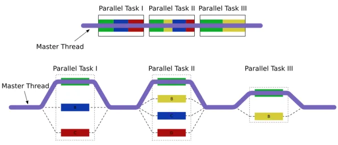
Thread Model of OpenMP
figure from Wikipedia: “OpenMP”
OpenMP directives OpenMP directives
• are an extension of the language
• are created by writting special pre-processor commands into the source code, which are interpreted by a suitable compiler
• start with \#pragma omp followed by a keyword and optionally some arguments
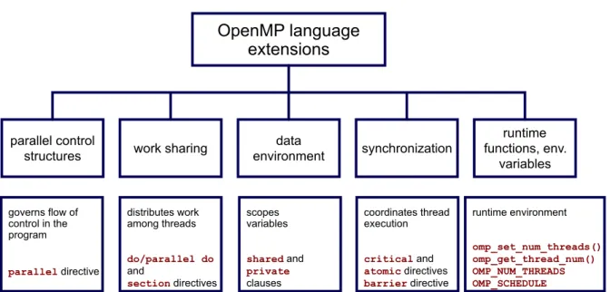
OpenMP Constructs
figure from Wikipedia: “OpenMP”
Scalar Product with OpenMP
# i f d e f _ O P E N M P
2 # include< omp . h >
# e n d i f
4
d o u b l e S c a l a r P r o d u c t ( std :: vector <double> a ,
6 std :: vector <double> b )
{
8 c o n s t int N = a . s i z e () ; int i ;
10 d o u b l e sum = 0 . 0 ;
# p r a g m a omp p a r a l l e l for
12 for ( i =0; i < N ;++ i ) sum += a [ i ] * b [ i ];
14 r e t u r n( sum ) ; }
Thread Initialisation
parallel starts a block which is run in parallel
for the iterations are distributed among the threads (often combined with parallel to one line\#pragma omp parallel for.
sections inside asectionsblock there are several independentsection blocks which can be executed independently.
if if an if is introduced in the thread initialisation command, the block is only executed in parallel if the condition afterif is true.
Synchronisation
critical mutual exclusion: the block is only executed by one thread at a time.
atomic same ascritical but tries to use hardware instructions
single the part inside thesingleblock is only executed by one thread. The other threads are waiting at the end of the block.
master the part inside themasterblock is only executed by the master thread. It is skipped by all other threads.
barrier each thread waits till all threads have reached the barrier
nowait usually threads wait at the end of a block. Ifnowaitis used they continue immediately Accessibility of Variables
shared All threads are accessing the same (shared) data.
private Each thread has its own copy of the data.
default is used to specify what’s the default behaviour for variables. Can beshared,private ornone.
reduction If reduction(operator,variable) is specified, each thread uses a local copy of variable but all local copies are combined with the operator operator at the end.
Possible operators are+ * - / & ^ | Scheduling of Parallel For-Loops
The distribution of the total number of iterations to the individual threads can be influenced by the argumentscheduleof the pragmafor. scheduleis followed in brackets by one of five parameters and optionally after a comma the chunk size. The chunk size has to be an integer value known at compile time. The default schedule is implementation dependent.
static chunks are distributed at the beginning of the loop to the different threads.
dynamic each time a thread finishes its chunk it gets a new chunk.
guided the chunk size is proportional to the number of unassigned iterations divided by the number threads (i.e. chunk size is getting smaller with time).
runtime scheduling is controlled by the runtime variableOMP_SCHEDULE. It is illegal to specify a chunk size.
auto scheduling is done by the compiler and/or runtime environment.
# d e f i n e C H U N K _ S I Z E 10
2 # p r a g m a omp p a r a l l e l for s c h e d u l e ( dynamic , C H U N K _ S I Z E )
Better Scalar Product with OpenMP
# i f d e f _ O P E N M P
2 # include< omp . h >
# e n d i f
4
d o u b l e S c a l a r P r o d u c t ( std :: vector <double> a ,
6 std :: vector <double> b )
{
8 c o n s t int N = a . s i z e () ; int i ;
10 d o u b l e sum = 0.0 , t e m p ;
# p r a g m a omp p a r a l l e l for s h a r e d ( a , b , sum ) p r i v a t e( t e m p )
12 for ( i =0; i < N ;++ i ) {
14 t e m p = a [ i ] * b [ i ];
# p r a g m a omp a t o m i c
16 sum += t e m p ;
}
18 r e t u r n( sum ) ; }
Improved Scalar Product with OpenMP
1 # i f d e f _ O P E N M P
# include< omp . h >
3 # e n d i f
5 d o u b l e S c a l a r P r o d u c t ( std :: vector <double> a , std :: vector <double> b )
7 {
c o n s t int N = a . s i z e () ;
9 int i ;
d o u b l e sum = 0 . 0 ;
11 # p r a g m a omp p a r a l l e l for s h a r e d ( a , b ) r e d u c t i o n (+: sum ) for ( i =0; i < N ;++ i )
13 sum += a [ i ] * b [ i ];
r e t u r n( sum ) ;
15 }
Parallel Execution of different Functions
1 # p r a g m a omp p a r a l l e l s e c t i o n s {
3 # p r a g m a omp s e c t i o n {
5 A () ;
B () ;
7 }
# p r a g m a omp s e c t i o n
9 {
C () ;
11 D () ;
}
13 # p r a g m a omp s e c t i o n {
15 E () ;
F () ;
17 }
}
Special OpenMP Functions
There is a number of special functions which are defined inomp.h, e.g.
• int omp_get_num_procs();returns number of available processors
• int omp_get_num_threads();returns number of started threads
• int omp_get_thread_num(); returns number of this thread
• void omp_set_num_threads(int i);set the number of threads to be used
# i f d e f _ O P E N M P
2 # i f d e f _ O P E N M P
# include< omp . h >
4 # e n d i f
# include< i o s t r e a m >
6 c o n s t int C H U N K _ S I Z E =3;
8 int m a i n (v o i d) {
10 int id ;
std :: c o u t < < " T h i s c o m p u t e r has " < < o m p _ g e t _ n u m _ p r o c s () < < " p r o c e s s o r s " < <
std :: e n d l ;
12 std :: c o u t < < " A l l o w i n g two t h r e a d s per p r o c e s s o r " < < std :: e n d l ; o m p _ s e t _ n u m _ t h r e a d s (2* o m p _ g e t _ n u m _ p r o c s () ) ;
14
# p r a g m a omp p a r a l l e l d e f a u l t( s h a r e d ) p r i v a t e( id )
16 {
# p r a g m a omp for s c h e d u l e (static, C H U N K _ S I Z E )
18 for (int i = 0; i < 7; ++ i )
{
20 id = o m p _ g e t _ t h r e a d _ n u m () ;
std :: c o u t < < " H e l l o W o r l d f r o m t h r e a d " < < id < < std :: e n d l ;
22 }
# p r a g m a omp m a s t e r
24 std :: c o u t < < " T h e r e are " < < o m p _ g e t _ n u m _ t h r e a d s () < < " t h r e a d s " < < std :: e n d l ; }
26 std :: c o u t < < " T h e r e are " < < o m p _ g e t _ n u m _ t h r e a d s () < < " t h r e a d s " < < std :: e n d l ;
28 r e t u r n 0;
}
Output
1 T h i s c o m p u t e r has 2 p r o c e s s o r s A l l o w i n g two t h r e a d s per p r o c e s s o r
3 H e l l o W o r l d f r o m t h r e a d 1
H e l l o W o r l d f r o m t h r e a d H e l l o W o r l d f r o m t h r e a d 0
5 H e l l o W o r l d f r o m t h r e a d 0 H e l l o W o r l d f r o m t h r e a d 0
7 2 H e l l o W o r l d f r o m t h r e a d
1
9 H e l l o W o r l d f r o m t h r e a d 1 T h e r e are 4 t h r e a d s
11 T h e r e are 1 t h r e a d s
Compiling and Environment Variables
OpenMP is activated with special compiler options. If they are not used, the #pragma statements are ignored and a sequential program is created. For icc the option is -openmp, forgccit is -fopenmp
The environment variableOMP_NUM_THREADS specifies the maximal number of threads. The call of the functionomp_set_num_threadsin the program has precedence over the environment variable.
Example (with gcc and bash under linux):
gcc - O2 - f o p e n m p - o s c a l a r _ p r o d u c t s c a l a r p r o d u c t . cc
2 e x p o r t O M P _ N U M _ T H R E A D S =3 ./ s c a l a r _ p r o d u c t
References
[1] OpenMP Specification http://openmp.org/wp/openmp-specifications/
[2] OpenMP Tutorial in four parts http://www.embedded.com/design/multicore/201803777 (this is part four with links to part one to three)
[3] Very complete OpenMP Tutorial/Reference https://computing.llnl.gov/tutorials/openMP [4] Intel Compiler (free for non-commercial use) http://www.intel.com/cd/software/products/asmo-
na/eng/340679.htm
4 Basics of Parallel Algorithms Basic Approach to Parallelisation
We want to have a look at three steps of the design of a parallel algorithm:
Decomposition of the problem into independent subtasks to identify maximal possible paral- lelism.
Control of Granularity to balance the expense for computation and communication.
Mapping of Processes to Processors to get an optimal adjustment of logical communication structure and hardware.
4.1 Data Decomposition
Algorithms are often tied to a special data structure. Certain operations have to be done for each data object.
Example: Matrix addition C = A + B, Triangulation
aij
j
i
Matrix
tj
Triangulation
Data Interdependence
Often the operations for all data objects can’t be done simultaneously.
Example: Gauß-Seidel/SOR-Iteration with lexicographic numbering.
Calculations are done on a grid, where the calculation at grid point (i, j) depends on the gridpoints (i−1, j) and (i, j−1). Grid point (0,0) can be calculated without prerequisites. Only grid points on the diagonali+j=const can be calculated simultaneously.
Data interdependence complicates the data decomposition considerably.
00 11
00 11
0 1
0 1
0 1
00 11
00 11
00 11
00 11
00 11
00 11
00 11
00 11
00
0 1 2 3
11
4 i0 1 2 3 4 j
Increasing possible Parallelism
Sometimes the algorithm can be modified to allow for a higher data Independence.
With a different numbering of the unknowns the possible degree of parallelism for the Gauß- Seidel/SOR-iteration scheme can be increased:
Every point in the domain gets a colour such that two neighbours never have the same colour. For structured grids two colours are enough (usually red and black are used). The unknowns of the same colour are numbered first, then the next colour. . ..
Red-Black-Ordering
The equations for all unknowns with the same colour are then independent of each other.
For structured grids we get a matrix of the form A=
DR F E DB
However, while such a matrix transformation does not affect the convergence of solvers like Steepest-Descent or CG (as they only depend on the matrix condition) it can affect the convergence rate of relaxation methods.
Functional Decomposition
Functional decomposition can be done, if different operations have to be done on the same data set.
Example: Compiler A compiler consists of
• lexical analysis
• parser
• code generation
• optimisation
• assembling
Each of these steps can be assigned to a separate process. The data can run through this steps in portions. This is also called “Macro pipelining”.
Irregular Problems
For some problems the decomposition cannot be determined a priory.
Example: Adaptive Quadrature of a functionf(x)
The choice of the intervals depends on the functionf and results from an evaluation of error predictors during the calculation.
f (x)
4.2 Agglomeration
Agglomeration and Granularity
The decomposition yields the maximal degree of parallelism, but it does not always make sense to really use this (e.g. one data object for each process) as the communication overhead can get too large.
Several subtasks are therefore assigned to each process and the communication necessary for each subtask is combined in as few messages as possible. This is called “agglomeration”. This reduces the number of messages.
The granularity of a parallel algorithm is given by the ratio granularity= number of messages
computation time Agglomeration reduces the granularity.
Example: Gridbased Calculations
Each process is assigned a number of grid points. Initerative calculations usually the value at each node and it’s neighbours is needed. If there is no interdependence all calculations can be done in parallel. A process withN grid points has to do O(N) operations. With the partition it only needs to communicate 4√
N boundary nodes. The ratio of communication to computation costs is therefore O(N−1/2) and can be made arbitrarily small by increasingN. This is calledsurface-to-volume-effect.
ProcessΠ
4.3 Mapping of Processes to Processors Optimal Mapping of Processes to Processors
The set of all process Π forms a undirected graphGΠ= (Π, K). Two processes are connected if they communicate.
The set of processors P together with the communication network (e.g. hypercube, field, . . .) also forms a graph GP = (P, N).
If we assume |Π| = |P|, we have to choose which process is executed on which processor.
In general we want to find a mapping, such that processes which communicate are mapped to proximate processors. This optimisation problem is a variant of thegraph partitioning problem and is unfortunatelyN P-complete.
As the transmission time in cut-through networks of state-of-the-art parallel computers is nearly independent of the distance, the problem of optimal process to processor mapping has lost a bit of it’s importance. If many processes have to communicate simultaneously (which is often the case!), a good positioning of processes is still relevant.
4.4 Load Balancing
Load Balancing: Static Distribution
Bin Packing At beginning all processors are empty. Nodes are successively packed to the processor with the least work. This also works dynamically.
Recursive Bisection We make the additional assumption, that the nodes have a position in space. The domain is split into parts with an equal amount of work. This is repeated recursively on the subspaces.
same
amount of work
4.5 Data Decomposition of Vectors and Matrices Decomposition of Vectors
A vectorx∈RN is a ordered list of numbers where each indexi∈I={0, . . . , N −1} is associated with a real numberxi.
Data decomposition is equivalent with a segmentation of the index seti in I= [
p∈P
Ip, withp6=q⇒Ip∩Iq =∅,
whereP denotes the set of processes. For a good load balancing the subsetsIp,p∈P should contain equal amounts of elements.
To get a coherent index set ˜Ip={0, . . . ,|Ip| −1} we define the mappings p: I→P and
µ: I→N
which reversibly associate each indexi ∈ I with a process p(i)∈P and a local indexµ(i) ∈I˜p(i): I3i7→(p(i), µ(i)).
The inverse mapping µ−1(p, i) provides a global index to each local indexi∈I˜p and process p∈P i.e. p(µ−1(p, i)) =pandµ(µ−1(p, i)) =i.
Common Decompositions: Cyclic
p(i) = i%P µ(i) = i÷P
÷denotes an integer division and % the modulo function.
I: 0 1 2 3 4 5 6 7 8 9 10 11 12 p(i) : 0 1 2 3 0 1 2 3 0 1 2 3 0 µ(i) : 0 0 0 0 1 1 1 1 2 2 2 2 3 e.g. I1= {1,5,9},
I˜1= {0,1,2}.
Common Decompositions: Blockwise
p(i) =
i÷(B+ 1) ifi < R(B+ 1) R+ (i−R(B+ 1))÷B else
µ(i) =
i%(B+ 1) ifi < R(B+ 1) (i−R(B+ 1)) %B else
with B=N÷P and R=N%P
I: 0 1 2 3 4 5 6 7 8 9 10 11 12 p(i) : 0 0 0 0 1 1 1 2 2 2 3 3 3 µ(i) : 0 1 2 3 0 1 2 0 1 2 0 1 2 e.g. I1= {4,5,6},
I˜1= {0,1,2}.
Decomposition of Matrices I
With a matrix A ∈ RN×M a real number aij is associated with each tupel (i, j) ∈ I ×J, withI ={0, . . . , N−1} andJ ={0, . . . , M −1}.
To be able to represent the decomposed data on each processor again as a matrix, we limit the decomposition to the one-dimensional index setsI and J.
We assume processes are organised as a two-dimensional field:
(p, q)∈ {0, . . . , P−1} × {0, . . . , Q−1}.
The index setsI,J are decomposed to I =
P−1
[
p=0
Ip and J =
Q−1
[
q=0
Jq
Decomposition of Matrices II
Each process (p, q) is responsible for the indices Ip×Jq and stores it’s elements locally as R( ˜Ip×J˜q)-matrix.
Formally the decompositions ofI and J are described as mappingsp and µplus q and ν: Ip={i∈I|p(i) =p}, I˜p={n∈N| ∃i∈I:p(i) =p ∧µ(i) =n}
Jq={j∈J |q(j) =q}, J˜q ={m∈N| ∃j∈J :q(j) =q ∧ ν(j) =m}
Decomposition of a 6×9 Matrix to 4 Processors
P= 1,Q= 4 (columns),J: cyclic:
0 1 2 3 4 5 6 7 8 J
0 1 2 3 0 1 2 3 0 q
0 0 0 0 1 1 1 1 2 ν
. . . . . . . . . . . . . . . . . . . . . . . . . . .
. . . . . . . . . . . . . . . . . . . . . . . . . . .
. . . . . . . . . . . . . . . . . . . . . . . . . . .
. . . . . . . . . . . . . . . . . . . . . . . . . . .
. . . . . . . . . . . . . . . . . . . . . . . . . . .
. . . . . . . . . . . . . . . . . . . . . . . . . . .
P= 4,Q= 1 (rows),I: blockwise:
0 0 0 . . . . . . . . . . . . . . . . . . . . . . . . . . .
1 0 1 . . . . . . . . . . . . . . . . . . . . . . . . . . .
2 1 0 . . . . . . . . . . . . . . . . . . . . . . . . . . .
3 1 1 . . . . . . . . . . . . . . . . . . . . . . . . . . .
4 2 0 . . . . . . . . . . . . . . . . . . . . . . . . . . .
5 3 0 . . . . . . . . . . . . . . . . . . . . . . . . . . .
I p µ
P= 2,Q= 2 (field),I: cyclic,J: blockwise:
0 1 2 3 4 5 6 7 8 J
0 0 0 0 0 1 1 1 1 q
0 1 2 3 4 0 1 2 3 ν
0 0 0 . . . . . . . . . . . . . . . . . . . . . . . . . . .
1 1 0 . . . . . . . . . . . . . . . . . . . . . . . . . . .
2 0 1 . . . . . . . . . . . . . . . . . . . . . . . . . . .
3 1 1 . . . . . . . . . . . . . . . . . . . . . . . . . . .
4 0 2 . . . . . . . . . . . . . . . . . . . . . . . . . . .
5 1 2 . . . . . . . . . . . . . . . . . . . . . . . . . . .
I p µ
Optimal Decomposition
There is no overall best solution for the decomposition of matrices and vectors!
• In general a good load balancing is achieved if the subsets of the matrix are more or less quadratic.