High statistics lattice study of stress tensor correlators in pure SU( 3 ) gauge theory
Sz. Borsányi,1Z. Fodor,1,2,3M. Giordano,3S. D. Katz,3A. Pásztor,1C. Ratti,4A. Schäfer,5K. K. Szabó,1,2and B. C. Tóth1
1University of Wuppertal, Department of Physics, Wuppertal D-42097, Germany
2Jülich Supercomputing Centre, Jülich D-52425, Germany
3Eötvös University, Budapest 1117, Hungary
4Department of Physics, University of Houston, Houston, Texas 77204, USA
5University of Regensburg, Regensburg D-93053, Germany
(Received 19 March 2018; published 27 July 2018)
We compute the Euclidean correlators of the stress tensor in pureSUð3ÞYang-Mills theory at finite temperature at zero and finite spatial momenta with lattice simulations. We perform continuum extrapolations usingNτ¼10, 12, 16, 20 lattices with renormalized anisotropy 2. We use these correlators to estimate the shear viscosity of the gluon plasma in the deconfined phase. ForT¼1.5Tc, we estimate η=s¼0.17ð2Þusing an ansatz motivated by hydrodynamics.
DOI:10.1103/PhysRevD.98.014512
I. INTRODUCTION
Since relativistic hydrodynamics is quite successful in the interpretation of heavy ion experiments[1–5], it would be of great interest to calculate the shear viscosity of the quark gluon plasma from first principles.
In classical transport theory, the shear viscosity to entropy density ratio for a dilute gas at temperature T is η=s∼Tlmfpv¯∼Tnσv¯, wherelmfpis the mean free path,v¯ is the mean speed,nis the particle number density andσthe cross section. For a weakly interacting system,σis small, andη=s is expected to be large. In particular, for a free gas,η=sis infinite. On the other hand, for a strongly interacting system, η=s is expected to be small [6]. As heavy ion phenomenology points to a rather small viscosity[1–5], a nonperturbative calculation of the shear viscosity would be a great success.
One possible route to determine the viscosity is through the Kubo formula, relating transport coefficients to the zero-frequency behavior of spectral functions. The relevant Kubo formula for the shear viscosity is
ηðTÞ ¼πlim
ω→0lim
k→0
ρijijðω;k; TÞ
ω ; ð1Þ
whereρijijðω;k; TÞis the spectral function corresponding to the energy momentum tensor at the specified spatial
indices i≠j. The direction of the momentum is j. In this paper, we will assume without any loss of generality, that the external momentum is in the 3rd direction, while the zeroth direction is the (Euclidean) time. By choosing a matchingiindex we will consider the compo- nentρ1313ðω;k; TÞ.
In general, the correlator of the energy momentum tensor Tμν is given in Euclidean spacetime as
Cμν;ρσðτ;x⃗ Þ ¼ Z
hTμνðτ0;x⃗0ÞTρσðτ0þτ;x⃗0þx⃗ Þidτ0dx⃗0; ð2Þ
which is a direct observable on the lattice. Its Fourier transform is related to the spectral function by an integral transform
Cμν;ρσðτ;qÞ ¼ Z ∞
0 dωρμν;ρσðω;q; TÞKðω;τ;TÞ; ð3Þ with the kernel
Kðω;τ;TÞ ¼coshðωðτ−1=ð2TÞÞÞ
sinhðω=ð2TÞÞ : ð4Þ Both early [7–9]and more recent[10]lattice studies of the viscosity used the Kubo formula(1). In this approach the integral transform(3)has to be inverted. ForT ≫ωthe kernel behaves likee−ωτ, i.e., our task is similar to inverting a Laplace transform numerically. It is well known that such an approach is bound to face great difficulties. There are two interrelated problems:
(1) Equation(3)is a Fredholm equation of the first kind, which for most kernels very ill-posed. The difficulty Published by the American Physical Society under the terms of
the Creative Commons Attribution 4.0 International license.
Further distribution of this work must maintain attribution to the author(s) and the published article’s title, journal citation, and DOI. Funded by SCOAP3.
can intuitively be compared to the process of de- blurring an image. Also, in particular, both the Laplace kernel, and our kernelKðω;τ;TÞare known to lead to a very ill-conditioned inverse problem[11].
(2) For the particular case of the viscosity, the signal in the stress-energy tensor is strongly dominated by the high frequency part of the spectral function [12].
This makes reconstruction even harder as the blur- ring character of the integral transform (point 1) mixes the contributions from the high and lowωpart of the spectral function in the measured Euclidean correlator.
To see how bad a particular inversion problem is, it is very instructive to look at the spectral function for the free theory, as this will correspond to the asymptotic behavior of the spectral function in the continuum theory, because of asymptotic freedom. To get the asymptotic behavior up to a constant, one only has to perform simple dimensional analysis. Forρ1313this leads to an asymptoticω4behavior, making the UV contamination especially severe.
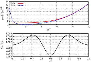
To see an honest illustration of these problems for ρ1313∼ω4, look at Fig. 1, where we illustrate how insensitive the Euclidean correlator is to the IR features of the spectral function. There we show two different spectral functions, with a factor of 10 difference in the viscosity, that nevertheless lead to subpercent differences in the corresponding Euclidean correlators. The two mock spectral functions in Fig. 1 are actually both physically motivated. The featureless spectral function (#1 in Fig.1) is reminiscent of the one obtained from calculations inN ¼4 SYM theory, with AdS=CFT methods [13], while the spectral function exhibiting a Lorentzian peak at ω¼0 is reminiscent of the kind of results one obtains from
leading log kinetic theory calculations in QCD itself[14].
Since the AdS=CFT calculation is a strong coupling calculation in the wrong theory, while the kinetic theory calculation is a calculation in the wrong regime of QCD, we do not knowa prioriwhich type of spectral function we can expect for QCD in the phenomenologically relevant tem- perature range, so a fully controlled calculation of the viscosity from the Kubo formula would necessarily need to distinguish between these two scenarios.
Note that for Fig. 1 we assumed that the asymptotic behavior of the spectral function is known completely accurately and there are no features of the spectral function at intermediate frequencies (e.g., no glueballs or remnants of melted glueballs). Though there has been progress in perturbative calculations of the UV part of the spectral functions[15–17], these assumptions are optimistic. Still, the fact that under these assumptions an order of magnitude difference in the viscosity leads to less than 1% difference in the Euclidean correlators nicely illustrates our point.
The bottom line of this discussion is that, for a credible lattice estimate of the viscosity, a high level of precision is necessary for the Euclidean correlators, especially if we want to use Eq.(1), as was done in Refs.[7–10,18].
The situation is much better for the correlators of conserved charges, appearing in the electric conductivity[19–22]and heavy quark diffusion[23–26]calculations. In those cases, the spectral function at largeωonly grows likeω2, making the UV contamination problem less severe. It was an important realization of Refs. [11,27] that even for the case of the shear viscosity, the asymptotic ω4 behavior can be made better, onlyω2, by utilizing the following Ward identity,
−ω2ρ0101¼q2ρ1313; ð5Þ and using the ρ0101 correlator, instead of the ρ1313. This would make the asymptotic behavior of the shear viscosity spectral function only as bad as that of the electric conduc- tivity. But there are crucial differences as well. In the continuum, we have the thermodynamic identity [28]
hT01T01iðτ;q¼0Þ=T5¼s=T3. This means that we need nonzero momenta to obtain information about the viscosity from this correlator.
Even with this knowledge, the calculation of the vis- cosity is still much more difficult than that of the electric conductivity. The source of the difficulty is the fact that the stress-energy tensor correlators CðτÞ have a quickly degrading signal as τ is increased beyond a few lattice spacings. Usually, the width of the distribution for these observables in a Monte Carlo simulation is much larger than the value, at least near the middle pointτT¼1=2, the very point where the correlator has its highest sensitivity to transport. Thus, the physically most relevant quantity is evaluated as an average of wildly fluctuating contributions (with fluctuating sign), which is typically the characteristic of a sign problem.
0 2 4 6 8 10 12 14
0 2 4 6 8 10
ρ(ω) / (ω T3)
ω/T SF #1
SF #2
0.992 0.994 0.996 0.998 1 1.002 1.004 1.006 1.008
0.1 0.2 0.3 0.4 0.5 0.6 0.7 0.8 0.9
C1 / C2
τT
FIG. 1. The Euclidean correlator corresponding to the spectral function appearing in Eq.(1)is very insensitive to its IR features.
To illustrate this, we show two different spectral functions, with the same UV, but different IR features (top) and the ratio of the corresponding Euclidean correlators (bottom). The viscosities are different by a factor of 10, but the Euclidean correlators differ by less than 1%.
For the quenched case this problem can be ameliorated by using the multilevel algorithm [29,30]. This algorithm depends crucially on the locality of the action, and therefore it proved to be hard to generalize for dynamical fermions.
Some progress in this regard has been made recently in [31,32]. Nevertheless, at least in the quenched case, high statistical precision can be achieved via the multilevel algorithm.
The study of cutoff effects of these correlators is rather limited in the literature. The tree level improvement coefficients for the plaquette action and two different discretizations of Tμν where calculated in [33]. So far, no calculations of these correlators are available with three lattice spacings in the scaling regime.
In this paper, we take steps towards achieving the high precision necessary for the calculation of the shear viscos- ity, by investigating several technical aspects of such a calculation, namely,
(i) Utilizing a different gauge action, the tree level Symanzik-improved action, as opposed to the pla- quette action used in previous studies.
(ii) Studing the continuum limit behavior by simulating at different values of the lattice spacingNt¼10, 12, 16 and 20.
(iii) Calculating the w0 scale with high precision.
(iv) Using the Wilson flow for anisotropy tuning, as advertised in [34].
(v) Using shifted boundary conditions for the renorm- alization of the energy momentum tensor, a tech- nique that was worked out for the isotropic case in [35]. Here, we utilize it for an anisotropic lattice.
(vi) Calculating the tree-level improvement coefficients for the Symanzik-improved gauge action.
Throughout this paper, we will mostly focus on the calculation of the energy-momentum tensor, and not the inversion method for reconstructing the spectral function.
We believe this to be an important first step. Before the inversion can be done, one needs to have reliable results for the correlator itself. Nevertheless, in the end we give an estimate of the viscosity, using a similar hydrodynamics motivated fit ansatz as some previous studies [11].
II. LATTICE CALCULATION OF THE CORRELATORS
Our calculation uses the tree-level Symanzik-improved gauge-action,
Stli¼βX
n
X
μ<ν
λμλν
λμ¯λν¯
1− 1
NcRe trUμνðnÞ
;
UμνðnÞ ¼c0Wμνðn;1;1Þ þc1Wμνðn;2;1Þ þc1Wμνðn;1;2Þ;
ð6Þ where β¼2Ng2c. μ¯ and ν¯ are the complementer indices forμandν, such thatμ¯ <ν¯ and the four indicesμ;ν;μ¯;ν¯
are a permutation of 0,1,2,3. HereWμνðn;a; bÞare Wilson loops around rectangulara×bpaths. Finally, c0¼53and c1¼−121.
The anisotropy parameters are λ1¼λ2¼λ3¼1, λ4¼ξ0, with ξ0 the bare anisotropy. For our study we use anisotropic lattices with renormalized anisotropy ξR¼2. For anisotropy tuning we use the Wilson flow technique introduced in[34]. The procedure for anisotropy tuning will be detailed later.
We use a multilevel algorithm (more precisely, a two- level algorithm[36]) to reduce errors near τT¼0.5.
We use the clover discretization of the energy momen- tum tensor, mainly because the center of the operator is always located on a site, therefore the separation of the operators is always an integer in lattice units. If one were to use the plaquette discretization, there would be a compo- nent that is defined for integer separations and one that is defined for half integer separations, and one would need an interpolation to add them together. This would lead to the appearance of a systematic error coming from the inter- polation, that we want to avoid.
Following the line of previous studies, we use the two- level algorithm, but now with a tree-level Symanzik improvement. [37] Thus we have thick layers (having a width of a full temporal lattice spacing) between the blocks in the inner update.
We have ensembles at two different temperatures,1.5Tc
and2Tc, and the following lattice geometries: Nz×N2y× Nt¼80×202×20, 64×162×16, 48×122×12, 40×102× 10. The long spatial direction is needed so that we can have small spatial momenta, to justify our hydrodynamics-moti- vated fit ansatz below.
A. Statistics
As was explained in the Introduction, the correlators are needed to a very high precision, if one wants to have useful information on transport. In the pureSUð3Þtheory this can be achieved by using a multilevel algorithm[29]and high statistics. Earlier lattice studies of the viscosity[7–10,18]
also use a multilevel algorithm.
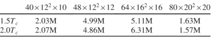
The main difference is—apart from the higher statistical precision—that we are working with four different lattice spacings, which allows us to study the correlators in the continuum limit. Our statistics are summarized in TableI.
TABLE I. Number of measurements (millions) of the energy- momentum tensor correlators at the simulation points. Between every measurement, there are 100 regular updates and 500 inner multilevel updates.
40×122×10 48×122×12 64×162×16 80×202×20
1.5Tc 2.03M 4.99M 5.11M 1.63M
2.0Tc 2.07M 4.86M 6.31M 1.57M
The relative statistical precision of our lattice data is shown in TableII.
B. Anisotropy tuning and scale setting
To fix the anisotropy we use the method introduced in [34]. The bare anisotropyξ0ðβÞis tuned so thatξR≡2. For the tuning, we define aspatial and a temporalw0 scale,
τ d
dττ2hEssðτÞi
τ¼w20;s ¼0.15; ð7Þ
τ d
dττ2hEtsðτÞi
τ¼w20;t ¼0.15; ð8Þ with
EssðτÞ ¼1 4
X
x;i≠j
F2ijðx;τÞ; ð9Þ
EstðτÞ ¼ξ2R
1 2
X
x;i
F2i4ðx;τÞ: ð10Þ To tune the anisotropy, we use the following procedure:
(1) We simulate theSUð3Þtheory at fixedβand several bare anisotropies around our estimate [34], target- ing ξR¼2.
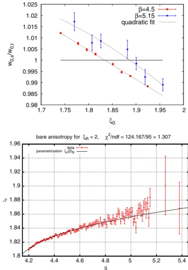
(2) We calculate the gradient flow using ξR¼2 and monitor w0;x=w0;t as a function of ξ0 (see Fig. 2).
The correct tuning of the anisotropy is achieved whenw0;x=w0;t¼1.
(3) Theξ0ðβÞdata set is fitted with a Pad´e formula. The fitted curve is plotted also in Fig. 2. Our para- metrization reads
ξ0ðβÞ ¼2.0
1þ6 β
−0.0578007þ0.2255046=β 1.0−3.94044=β
:
ð11Þ We likewise fit w0ðβÞ, with a parametrization that inter- polates smoothly between the two-loop running of the coupling and the lattice data,
w0ðβÞ ¼exp
− b1 2b20log
β 2Ncb0
þ β
4Ncb0
−3.51307817908059
− 1
−8.0963941698416þ2.36701001378353β
; ð12Þ
with b0¼11Nc=48π2, b1¼34N2c=768π4 and Nc ¼3. So far, we expressed the scale using w0. In order to be able to translate to the Tc scale, we have to determine the combination w0Tc in the continuum limit. We did this using four different (isotropic) actions (Wilson, tree-level Symanzik, Iwasaki and DBW2). With the exception of the last one, we found similar results using lattices up to Nτ ¼12 and a continuum limit using an N2τ as well as an N4τ term. The uncontrolled systematics of the DBW2 result is no surprise, this action is known to poorly sample topological sectors, see for e.g., [39].
In all cases,Tcwas defined by the peak of the Polyakov loop susceptibility. The summary plot for this study is shown in Fig. 3 For each action, the resulting jackknife error was very small. Therefore we use the spread between the Wilson, Symanzik and Iwasaki results as an error estimate instead, and use the Symanzik result (which lies central between the others) as mean. We conclude thatw0Tc ¼0.2535ð2Þ.
TABLE II. Relative statistical error of the 1313 correlators at zero momentum for our different simulation points.
40×122×10 48×122×12 64×162×16 80×202×20
1.5Tc .2% .2% .3% 1%
2.0Tc .3% .2% .4% 1%
0.98 0.985 0.99 0.995 1 1.005 1.01 1.015 1.02 1.025
1.7 1.75 1.8 1.85 1.9 1.95 2
w0,s/w0,t
ξ0
β=4.5 β=5.15 quadratic fit
1.8 1.82 1.84 1.86 1.88 1.9 1.92 1.94 1.96
4.2 4.4 4.6 4.8 5 5.2 5.4
ξ0
β
bare anisotropy for ξR = 2, χ2/ndf = 124.167/95 = 1.307
parametrization ξ0data(β)B
FIG. 2. Top: Anisotropy tuning with simulations at different bare anisotropies. The tuned bare anisotropy corresponds to w0;s=w0;t¼1. Bottom: Parametrization of the bare anisotropy used for our simulations.
C. Renormalization
The translational symmetry is broken on the lattice. As a result, renormalization factors appear between the lattice definition of the energy momentum tensor Tμν and the physical quantity. This factor depends on the action, the discretization scheme in theTμν observable and the lattice spacing (or the β parameter). Moreover, these factors are not the same for each component, since the off-diagonal (sextet), the diagonal (triplet), and the trace (singlet) correspond to different representations of the four- dimensional rotation group. On an isotropic lattice, one has three factors,
TRμν¼Z6T½6μνþZ3T½3μνþZ1ðT½1μν−T½1μνðT ¼0ÞÞ; ð13Þ where
T½6μν ¼ 1 g20
X
σ
FaμσFaνσ; ð14Þ
T½3μν¼δμν 1 g20
X
ρ
FaμρFaνρ−1 4
X
ρ;σ
FaρσFaρσ
; ð15Þ
T½1μν ¼δμν 1 g20
X
σ;ρ
FaρσFaρσ; ð16Þ
and there is no summation over μ and ν in the above formulas.
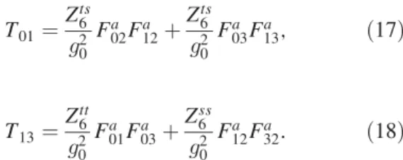
We use the clover discretization of Faμν and define our correlators from the sextet (off-diagonal) components. In the presence of anisotropy, the renormalization constantZ6 splits into three different renormalization constants:
T01¼Zts6
g20 Fa02Fa12þZts6
g20 Fa03Fa13; ð17Þ
T13¼Ztt6
g20Fa01Fa03þZss6
g20 Fa12Fa32: ð18Þ In our renormalization procedure, we get Zts6 from the thermodynamic identity(20), and we get the ratiosZss6=Zts6 andZtt6=Zts6 from shifted boundary conditions.
For an isotropic gauge action, the renormalization constants have been worked out with shifted boundary conditions in[35]. Using shifted boundary conditions with shift vectorξ⃗ ¼ ðξ1;ξ2;ξ3Þ ¼ ð1;1;1Þ, the off-diagonalT0i components develop a nonvanishing expectation value.
Since with this particular choice of the shift, the three spatial directions are equivalent, we haveT01¼T02¼T03. We note that this renormalization condition is very similar to the one used in[40], where it was used for the second- order hydrodynamic coefficientκ. Imposing this condition gives
2Ztt6 1
g20Fa02Fa12¼2Zss6 1 g20Fa03Fa13
¼Zst6 1
g20ðFa01Fa21þFa03Fa23Þ: ð19Þ
Therefore, the ratiosZss6=Zts6 andZtt6=Zts6 can be calculated from a single simulation with L−10 ¼T
ffiffiffiffiffiffiffiffiffiffiffiffiffiffiffi 1þ j⃗ξj2 q
¼2T.
Thus, e.g., to renormalizeTμνin aNτ¼12simulation with ξR¼2, we make an auxiliary run on a 48×96×48×3 lattice with the same bare parameters. The resulting factors will depend onβandNτ. The method requires thatNτ=4is an integer. We observe a1=N2τ scaling of bothZss6=Zts6 and Ztt6=Zts6. For the renormalization ofNτ ¼10we can there- fore use an interpolation inNτ. Our simulated results on the renormalization factors can be seen in Fig.4.
The overall constant Zts6 can be determined from the following thermodynamic identity[41]:
C0101ðτ;q¼0Þ=T5¼−s=T3: ð20Þ
This can be used for renormalization by requiring that the value ofC0101 at τT ¼0.5equals the continuum value of the entropy determined in[42]. We used the valuess=T3¼ 5.02and 5.57 for1.5Tcand2Tcrespectively. This identity also provides a way to estimate the order of magnitude of the discretization errors in C0101. Since in the continuum this correlator is independent ofτ, theτdependence of the correlator gives a very direct way to see discretization errors already on the finiteNτdata (for the case ofNt¼16, see Fig.6).
FIG. 3. Determination ofw0Tcfrom four different pureSUð3Þ actions.
III. RESULTS ON THE CORRELATORS A. Results at finiteNt
The 13 channel correlators can be seen in Fig.5, while the results for the 01 channel can be seen in Fig.6.
We note here, that trying a simple featureless ansatz ρ1313¼AωþBω4on ourNt¼20lattices (T ¼1.5Tc) for τ≥6=10 and q¼0 we get χ2=ndof¼3.8=3, while an ansatz with an infinitely sharp transport peak ρ1313¼ AδðωÞωþBω4 gives χ2=ndof¼5.7=3, giving a slight preference to the featureless scenario that we will later use in our more detailed analysis, while not yet ruling the sharp transport peak scenario out.
For the 01 channel, in the continuum, the correlator for zero spatial momentum should be a constant, equal to the entropy. The renormalization condition we used for this correlator is simply that at the middle point, τT¼1=2 it should equal the continuum value of−s=T3. How different the correlators value is for τT ≠1=2 is some kind of measure of the cutoff effects. As we already discussed, we expect the 01 channel to have smaller cutoff errors and also
to be more sensitive to transport, so this is the more important of the two correlators.
B. Continuum limit extrapolation
For the purpose of this paper we focus our discussion of the continuum limit extrapolation to the middle point of the correlatorsτT¼1=2. We choose this approach for several reasons:
(i) This is the most IR sensitive part of the correlators, therefore the most interesting part for studying transport.
(ii) This is the part of the correlator with the least amount of cutoff effects, therefore one has to control the continuum extrapolation of this first, before attempting to go to smaller separations in imaginary time.
0.61 0.615 0.62 0.625 0.63 0.635 0.64 0.645 0.65 0.655
4.5 4.6 4.7 4.8 4.9 5 5.1 5.2 5.3 5.4 Z6ss /Z6ts
β 32x64x32x2
48x96x48x3 64x128x64x4 80x160x80x5
1.6 1.62 1.64 1.66 1.68 1.7 1.72 1.74 1.76 1.78
4.5 4.6 4.7 4.8 4.9 5 5.1 5.2 5.3 5.4 Z6tt /Z6ts
β 32x64x32x2
48x96x48x3 64x128x64x4 80x160x80x5
FIG. 4. The renormalization factors Zss6=Zts6 (top) andZtt6=Zts6 (bottom) as obtained from our simulations with shifted boundary conditions with shift vectorξ⃗ ¼ ð1;1;1Þ.
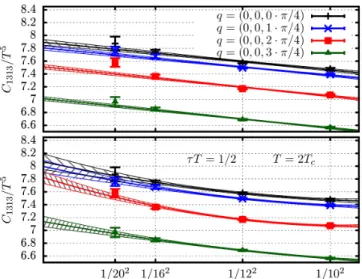
FIG. 5. The renormalized shear correlator C1313 at different lattice spacings and different spatial momenta. We also present a continuum estimate, that was produced by performing a spline interpolation of the finiteNtdata. We only present the continuum estimate in the range where theχ2 was acceptable.
FIG. 6. The renormalized shear correlatorC0101atNt¼16and for different spatial momenta for the temperatureT¼1.5Tc.
Notice, that the C1313 correlator is closely related to the τ derivative of the C0101 correlator:
d2C0101ðτ ¼1=2T;qÞ
dτ2 ¼
Z
dωω2ρ0101ðω;qÞ
sinhðβω2Þ ð21Þ C1313ðτ¼1=2T;qÞ ¼
Z
dω−ðω2=k2Þρ0101ðω;qÞ sinhðβω2Þ ð22Þ
C1313ðτ¼1=2T;qÞ ¼− 1 k2
d2C0101ðτ¼1=2T;qÞ
dτ2 ; ð23Þ as can be seen from a differentiation of the sum rule(3)and application of the Ward identity (5) respectively. Thus, taking theC1313ðτ;qÞandC0101ðτ;qÞcorrelators only at the valueτT ¼1=2already contains the leadingτdependence of C0101. Thus, we may continue with the extrapolation at τT ¼1=2.
We will attempt a continuum limit extrapolation both with and without tree-level improvement. The tree-level improvement coefficients are the result of a tedious, but straightforward computation. The numerical values of the improvement coefficients are summarized in AppendixB.
We will also attempt both linear and quadratic fits for the continuum limit extrapolation. Attempting a continuum limit extrapolation from ourNt¼10, 12, 16, 20 data yields the following behavior:
(i) In the 0101 channel, since one applies the renorm- alization condition (11) after the tree-level improve- ment, the continuum extrapolation is quite flat, regardless of whether one uses tree-level improve- ment or not.
(ii) A linear fit to theNt¼10, 12, 16, 20 lattices in the 1313 channel with and without tree-level improve- ment does not always yield consistent results within 1σ for the continuum limit extrapolation.
(iii) A quadratic fit to theNt¼10, 12, 16, 20 lattices in the 1313 channel with and without tree-level im- provement does yield consistent results, but then we have one degree of freedom less, so the error on the continuum is larger, roughly on the 2%–3% level.
(iv) Linear versus quadratic fits to the data obtained without tree-level improvement are not consistent within1σ for the 1313 channel.
(v) Linear versus quadratic fits to the tree-level im- proved data are closer, but still not consistent within 1σ for the 1313 channel.
This behavior can be visually observed in Figs.7–9where the linear and quadratic extrapolations are shown.
From this analysis, we conclude that from our present data, the continuum extrapolation has error bars on the few
FIG. 7. Continuum limit extrapolation ofC1313atτT¼1=2and T¼2Tc. The tree-level improvement was not applied to the data.
Top: linear fit; Bottom: quadratic fit.
FIG. 8. Continuum limit extrapolation ofC1313atτT¼1=2and T¼2Tc with the tree-level improvement applied to the lattice data. Top: linear fit; Bottom: quadratic fit.
FIG. 9. Continuum limit extrapolation ofC0101atτT¼1=2and T¼2Tc. Top: linear fit; Bottom: quadratic fit.
percent level, for both channels. The results for the three- point linear fits are summarized in TableIII.
C. Finite volume effects at tree level
From the tree-level calculation, we can estimate the finite volume effects on the UV contribution to the correlators.
For the volumes used for our simulations, i.e., LxT¼ LyT ¼2 and LzT ¼8 we calculated the tree-level (UV) contribution of the spectral function in Appendix B. The relative deviation from the infinite volume contribution is shown in TableIV. Thus, the tree-level finite volume effect on the observables considered here is on the 10% level.
While 10% error on the final viscosity is probably harmless at this point, it may shift the relative weight of the UV and IR contributions. It is important to note, that the finite volume correction depends very weakly onqand forC0101 it weakly depends onτ, too. Thus, in the viscosity fits the volume dependence approximately factorizes, and it affects only the value of thecparameter in Eq.(24). The values we
quote later will correspond to the raw fit, which is expected to be roughly 10% below the infinite volume value.
IV. ESTIMATING THE VISCOSITY
To get an educated guess on the viscosity, one needs to assume an ansatz. Here, we assume a very simple hydro- dynamics plus tree-level ansatz for the spectral function, corresponding to the featureless scenario in Fig.1:
Cμνμνðτ;qÞ ¼c Z ∞
jqj ρtree levelμνμν ðω;qÞKðτ;ωÞdω þ
Z ∞
0 ρhydroμνμνðω;q;η=sÞKðτ;ωÞdω ð24Þ The hydrodynamic predictions for the spectral function are written out in AppendixA. The tree-level spectral function is taken to be the one at infinite volume and in the continuum. Notice that the integral inωfor this UV part is cut off at ω¼ jqj in the IR. The part at lower ω is responsible for the hydrodynamical behaviour, which is taken into account by the other term. Actually, the free gas formula would give an infinite contribution to the viscosity.
The formulas for the continuum tree-level spectral function can be found in Ref. [27] and are also summarized in AppendixB.
We introduce a constant c in front of the spectral function. We do so to account in a simple way for higher-order and also finite volume corrections. The assumption that all of these effects can be put into a single constant is a very strong one. One hint that it might be a good estimate is given by TableII, where we have the finite volume correction factors for different correlators.
This model has two free parameters[43], the factorcin front of the tree-level correlator, and the shear viscosity to entropy ratio η=s may be contaminated by higher-order contributions, as well. Clearly, our estimate of the viscosity is correct only in the range of validity of this simple model for the spectral function. In the following, we will work out how data constrain the model parameters. Assuming that our system is within the model’s range of validity, we can make a quantitative statement on the shear viscosity.
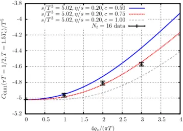
A. Sensitivity to model parameters
Before describing the fitting procedure let us show how the different model parameters influence the observables considered here. Since it is the more interesting quantity, our discussion here will focus onC0101. Figures10and11 concentrate on changing one of the parameters,cor η=s, respectively. From these pictures the conclusion one can draw is thatC0101, while certainly sensitive to the hydro- dynamic parameter η=s, is also sensitive to the UV parameterc. This is not surprising, but it is a big advantage compared to theC1313 correlator, where the sensitivity to η=sis smaller. Still, one has to acknowledge that while this TABLE III. Values of the correlators in the continuum. The
error bar includes statistical errors, as well as systematic errors coming from the linear vs quadratic continuum fit, and continuum extrapolation with and without tree-level improvement.
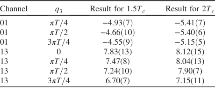
Channel q3 Result for1.5Tc Result for 2Tc
01 πT=4 −4.93ð7Þ −5.41ð7Þ
01 πT=2 −4.66ð10Þ −5.40ð6Þ 01 3πT=4 −4.55ð9Þ −5.15ð5Þ
13 0 7.83(13) 8.12(15)
13 πT=4 7.47(8) 8.04(13)
13 πT=2 7.24(10) 7.90(7)
13 3πT=4 6.70(7) 7.15(11)
TABLE IV. Finite volume corrections at tree level for the different correlators.
Channel τT q3 (Finite vol.)/(infinite vol.)
01 1=2 0 0.90
01 1=2 πT=4 0.92
01 1=2 πT=2 0.90
01 1=2 3πT=4 0.89
13 1=2 0 0.89
13 1=2 πT=4 0.90
13 1=2 πT=2 0.90
13 1=2 3πT=4 0.90
01 1=4 0 0.90
01 1=4 πT=4 0.92
01 1=4 πT=2 0.91
01 1=4 3πT=4 0.90
13 1=4 0 0.99
13 1=4 πT=4 0.99
13 1=4 πT=2 0.99
13 1=4 3πT=4 0.99
is a pretty useful quantity, because of the sensitivity to both parameters, it is not enough to constrain the value ofcand η=stogether. To do that one has to consider in addition theτ dependence ofC0101, or equivalently, the correlatorC1313at τ¼0, which, as we have already shown, corresponds to the second τ derivative of C0101.
B. Fits at finiteNt
We will present two different fits for the parameter c andη=s. First we study onlyC0101as a function ofτandq atNτ ¼16. This approach is similar to what was used in earlier publications, where only data at one finite Nt were available. Our choice of the channel C0101 is moti- vated by the smaller cutoff errors compared to C1313, as well as its higher sensitivity to the transport part of the spectral function. We constrain our fits to the range
τT ∈½0.3;0.5. This range is motivated by two observa- tions: i) the quantityC0101ðτ;q¼0Þ, which is, in principle, independent ofτ in the continuum, is indeed constant for Nt¼16 in this range (see Fig. 6); ii) the finite volume corrections at tree level are alsoτindependent in this range.
The latter fact motivates the assumption that most finite volume effects can be captured by a modified value of the cparameter.
T η=s c
1.5Tc 0.178(15) 0.60(6)
2.0Tc 0.157(13) 0.63(7)
Here the error includes statistical errors, as well as systematic errors coming from the choice of τmin¼ 5.=16 or 6.=16 and qmax¼2π=4 or qmax¼3π=4. These numbers are, of course, only valid once we assume our hydrodynamic ansatz.
The viscosity appears to be temperature independent from our analysis. Here we have to mention a serious drawback of our fit ansatz. It assumes that the hydrodynamic prediction for the spectral function, strictly valid only forω≪T, is also a good approximation for higher frequencies. This is true for N ¼4 SYM theory, where AdS=CFT can be used to calculate the spectral function [13]. Our ansatz cannot produce a quasiparticle peak, that would appear in weak coupling treatements of QCD, like kinetic theory[14,44,45].
This means that the physical mechanism that makes the viscosity diverge forT→∞, namely the sharpening of the peak inρ1313nearω¼0is missing from our ansatz. This implies that our ansatz can certainly not be used at very high temperatures, where the weak coupling calculation is trust- worthy, and even at intermediate temperatures we might underestimate the viscosity, effectively smearing out the transport peak by enforcing the ansatz in the data analysis.
This is a weakness shared by all previous lattice estimates of the shear viscosity, since they either use a very similar hydrodynamic ansatz, or the Backus-Gilbert method, in which case the base functions used for the reconstruction similarly prefer a featureless behavior, as opposed to a transport peak[11].
C. Fits on continuum data
For the second fit we consider theq3=ðπT=4Þ ¼0, 1, 2, 3 dependence ofC0101ðτT¼0.5ÞandC1313ðτT ¼0.5Þin the continuum. Our results are
T η=s c
1.5Tc 0.17(2) 0.63(3)
2.0Tc 0.15(2) 0.67(3)
Here, the error is statistical only. The systematic error coming from the choice of theτrange does not exist here, since we always use justτ ¼1=2. This fit uses the same hydrodynamic ansatz as discussed above.
FIG. 10. Effect of changing the UV parametercin the model on the correlator C0101 at τT¼1=2 for several different spatial momenta.
FIG. 11. Effect of changing the hydrodynamic parameterη=sin the model on the correlatorC0101atτT¼1=2for several different spatial momenta.
This is the first estimate of η=s using continuum extrapolated data. It is consistent with earlier estimates using a single lattice spacing [9,46].
V. SUMMARY
In this paper we studied the continuum behavior of the energy-momentum tensor correlators in pureSUð3Þgauge theory. We found cutoff errors at a few percent level for Nt¼16. For some quantities, namely C1313 andC0101 at several spatial momenta, andτT ¼1=2continuum extrapo- lation was possible. Out of these quantitiesC0101is actually sensitive to the transport part of the spectral function.
The achieved percent level precision of the data does not yet allow us to distinguish different scenarios for the spectral function. The statistical precision was already boosted by the multilevel algorithm on an anisotropic lattice. Despite recent efforts of using the gradient flow to measure energy-momentum tensor correlator[47,48]and the promising extension of the multilevel algorithm to full QCD [31] it is hardly possible to achieve even this precision with dynamical quarks. Thus, for the testing of the hydrodynamical model one has to seek for alternative methods.
Once, however, a model is postulated, it is possible to give a model-dependent estimate of the shear viscosity to entropy ratio. We gave the first estimate of this phenom- enologically important quantity from continuum extrapo- lated lattice data. Our estimate is in the same ballpark as earlier estimates based on finiteNt lattices.
ACKNOWLEDGMENTS
This project was funded by the DFG Grant No. SFB/
TR55. This work was partially supported by the Hungarian National Research, Development and Innovation Office— NKFIH Grants No. KKP126769 and No. K113034. An award of computer time was provided by the INCITE program. This research used resources of the Argonne Leadership Computing Facility, which is a DOE Office of Science User Facility supported under Contract No. DE- AC02-06CH11357. We acknowledge computer time on the QPACE machines [49] on the Wuppertal and Jülich sites. The authors gratefully acknowledge the Gauss Centre for Supercomputing (GCS) for providing computing time for a GCS Large-Scale Project on the GCS share of the supercomputer JUQUEEN at the Jülich Supercomputing Centre[50]. This material is based upon work supported by the National Science Foundation under Grants No. PHY-1654219 and No. OAC-1531814 and by the U.S. Department of Energy, Office of Science, Office of Nuclear Physics, within the framework of the Beam Energy Scan Theory (BEST) Topical Collaboration.
C. R. also acknowledges the support from the Center of Advanced Computing and Data Systems at the University of Houston.
APPENDIX A: PREDICTIONS OF HYDRODYNAMICS FOR THE
SPECTRAL FUNCTIONS
The combination of linearized relativistic hydrodynam- ics and linear response theory allows for a derivation of the low frequency behavior of the energy-momentum tensor correlators. For a nice derivation of these formulas, see the Appendix of [13]. Here, we just collect the relevant formulas in our notation, for easy reference. We assume the spatial momentum is in thezdirectionk¼ ð0;0; kÞ. In this case the spectral functions in the shear channel are:
−ρ0101
ω ¼η π
k2
ω2þ ðsTη k2Þ2 ðA1Þ ρ1313
ω ¼η π
ω2
ω2þ ðsTη k2Þ2; ðA2Þ wheresis the entropy,ηis the shear viscosity andTis the temperature. We use these formulas for both our finiteNτ and continuum data fits. The zero spatial momentum limit ofρ1313=ωis a constant equal toη=π, while the zero spatial momentum limit of theρ0101=ωis a delta function at the origin:
ρ1313 ω →1
2sTδðω−ϵÞ; ðA3Þ as can be easily shown using Eq. (A1). This is the hydrodynamic identity we utilize for our renormalization procedure. Formulas(A1) and(A2) are also the basis for the derivation of the Kubo formulas, like Eq.(1).
APPENDIX B: TREE-LEVEL SPECTRAL FUNCTION IN THE CONTINUUM
The leading-order perturbative result for the spectral function at high frequency is[27]
−ρðpertÞ0101 ¼ dA
8ð4πÞ2q2ðω2−q2ÞIðω; q; TÞ; ðB1Þ
Iðω; q; TÞ ¼θðω−qÞ Z 1
0 dz ð1−z4Þsinhðω=2TÞ coshðω=2TÞ−coshðqz=2TÞ þθð−ωþqÞ
Z ∞
1
ðz4−1Þsinhðω=2TÞ coshðω=2TÞ−coshðqz=2TÞ:
ðB2Þ The tree-level result in the ρpert1313 channel follows trivially using the Ward identity(5).
In our analysis, we only take the first part ω> q. The reason for that is that theω< qpart describes the transport properties of a free gas of gluons, and corresponds to an infinite viscosity. We therefore drop this term and substitute
it with the ansatz from hydrodynamics (which describes a strongly coupled system).
APPENDIX C: TREE-LEVEL IMPROVEMENT COEFFICIENTS
The formulas for the tree-level improvement are the result of a tedious but straightforward leading-order cal- culation. The resulting formulas still contain Matsubara sums, that can be easily evaluated numerically. For refer- ence, we include here the numerical values of the tree-level improvement coefficients relevant for our study.
mn qπ4T Nt CtlðNt¼infÞ=CtlðNtÞ
01 0 10 1.26852
01 0 12 1.19188
01 0 16 1.11254
01 0 20 1.07385
01 1 10 1.25721
01 1 12 1.18425
01 1 16 1.10833
01 1 20 1.07118
01 2 10 1.26208
01 2 12 1.18749
01 2 16 1.11007
(Table continued)
(Continued)
mn qπ4T Nt CtlðNt¼infÞ=CtlðNtÞ
01 2 20 1.07227
01 3 10 1.27067
01 3 12 1.19333
01 3 16 1.11328
01 3 20 1.07430
13 0 10 1.19957
13 0 12 1.15874
13 0 16 1.10223
13 0 20 1.06957
13 1 10 1.20054
13 1 12 1.15971
13 1 16 1.10297
13 1 20 1.07011
13 2 10 1.20329
13 2 12 1.16254
13 2 16 1.10515
13 2 20 1.07168
13 3 10 1.20742
13 3 12 1.16703
13 3 16 1.10869
13 3 20 1.07428
[1] D. Teaney, J. Lauret, and E. V. Shuryak,Phys. Rev. Lett.86, 4783 (2001).
[2] P. Romatschke and U. Romatschke, Phys. Rev. Lett. 99, 172301 (2007).
[3] P. Romatschke,Int. J. Mod. Phys. E19, 1 (2010).
[4] T. Schäfer and D. Teaney, Rep. Prog. Phys. 72, 126001 (2009).
[5] U. Heinz and R. Snellings,Annu. Rev. Nucl. Part. Sci.63, 123 (2013).
[6] P. K. Kovtun, D. T. Son, and A. O. Starinets,Phys. Rev. Lett.
94, 111601 (2005).
[7] F. Karsch and H. W. Wyld,Phys. Rev. D35, 2518 (1987).
[8] A. Nakamura and S. Sakai, Phys. Rev. Lett. 94, 072305 (2005).
[9] H. B. Meyer,Phys. Rev. D76, 101701 (2007).
[10] N. Astrakhantsev, V. Braguta, and A. Kotov,Eur. Phys. J.
Web Conf.137, 07003 (2017).
[11] H. B. Meyer,Eur. Phys. J. A47, 86 (2011).
[12] G. Aarts and J. M. Martinez Resco,J. High Energy Phys. 04 (2002) 053.
[13] D. Teaney,Phys. Rev. D74, 045025 (2006).
[14] J. Hong and D. Teaney,Phys. Rev. C82, 044908 (2010).
[15] Y. Schroder, M. Vepsalainen, A. Vuorinen, and Y. Zhu, J.
High Energy Phys. 12 (2011) 035.
[16] Y. Zhu and A. Vuorinen, J. High Energy Phys. 03 (2013) 002.
[17] A. Vuorinen and Y. Zhu,J. High Energy Phys. 03 (2015) 138.
[18] N. Astrakhantsev, V. Braguta, and A. Kotov,J. High Energy Phys. 04 (2017) 101.
[19] G. Aarts, C. Allton, J. Foley, S. Hands, and S. Kim,Phys.
Rev. Lett.99, 022002 (2007).
[20] H. T. Ding, A. Francis, O. Kaczmarek, F. Karsch, E. Laermann, and W. Soeldner,Phys. Rev. D83, 034504 (2011).
[21] G. Aarts, C. Allton, A. Amato, P. Giudice, S. Hands, and J.-I. Skullerud,J. High Energy Phys. 02 (2015) 186.
[22] H.-T. Ding, O. Kaczmarek, and F. Meyer,Phys. Rev. D94, 034504 (2016).
[23] P. Petreczky and D. Teaney, Phys. Rev. D 73, 014508 (2006).
[24] A. Jakovac, P. Petreczky, K. Petrov, and A. Velytsky,Phys.
Rev. D 75, 014506 (2007).
[25] S. Borsanyiet al.,J. High Energy Phys. 04 (2014) 132.
[26] A. Francis, O. Kaczmarek, M. Laine, T. Neuhaus, and H.
Ohno,Phys. Rev. D92, 116003 (2015).
[27] H. B. Meyer,J. High Energy Phys. 08 (2008) 031.
[28] See AppendixA.
[29] M. Luscher and P. Weisz,J. High Energy Phys. 09 (2001) 010.
[30] H. B. Meyer,J. High Energy Phys. 01 (2003) 048.
[31] M. Ce, L. Giusti, and S. Schaefer,Phys. Rev. D93, 094507 (2016).
[32] M. Ce, L. Giusti, and S. Schaefer,Phys. Rev. D95, 034503 (2017).
[33] H. B. Meyer,J. High Energy Phys. 06 (2009) 077.
[34] S. Borsanyi, S. Durr, Z. Fodor, S. D. Katz, S. Krieg, T.
Kurth, S. Mages, A. Schafer, and K. K. Szabo, arXiv:
1205.0781.
[35] L. Giusti and M. Pepe,Phys. Rev. D91, 114504 (2015).
[36] H. B. Meyer,J. High Energy Phys. 01 (2004) 030.
[37] Note, that this combination was already used in the literature for the calculation of static quark potentials[38].
[38] A. Mykkanen,J. High Energy Phys. 12 (2012) 069.
[39] T. A. DeGrand, A. Hasenfratz, and T. G. Kovacs,Phys. Rev.
D67, 054501 (2003).
[40] O. Philipsen and C. Schäfer,J. High Energy Phys. 02 (2014) 003.
[41] See AppendixA.
[42] S. Borsanyi, G. Endrodi, Z. Fodor, S. D. Katz, and K. K.
Szabo,J. High Energy Phys. 07 (2012) 056.
[43] The entropy is fixed from previous calculations of the equation of state.
[44] P. B. Arnold, G. D. Moore, and L. G. Yaffe,J. High Energy Phys. 11 (2000) 001.
[45] P. B. Arnold, G. D. Moore, and L. G. Yaffe,J. High Energy Phys. 05 (2003) 051.
[46] S. W. Mages, S. Borsányi, Z. Fodor, A. Schäfer, and K.
Szabó,Proc. Sci.LATTICE2014 (2015) 232.
[47] Y. Taniguchi, S. Ejiri, K. Kanaya, M. Kitazawa, A. Suzuki, H. Suzuki, and T. Umeda (WHOT-QCD),Eur. Phys. J. Web Conf.175, 07013 (2018).
[48] M. Kitazawa, T. Iritani, M. Asakawa, and T. Hatsuda,Phys.
Rev. D 96, 111502 (2017).
[49] H. Baier et al., Proc. Sci. LAT2009 (2009) 001, arXiv:
0911.2174.
[50] JUQUEEN: Ibm blue gene/q supercomputer system at the julich supercomputing centre, tech. rep.1 a1 (julich super- computing centre,http://dx.doi.org/10.17815/jlsrf-1-182015).