Pion distribution amplitude from Euclidean correlation functions:
Exploring universality and higher-twist effects
Gunnar S. Bali,1,2 Vladimir M. Braun,1 Benjamin Gläßle,1,3 Meinulf Göckeler,1Michael Gruber,1 Fabian Hutzler,1 Piotr Korcyl,1,4 Andreas Schäfer,1 Philipp Wein,1,* and Jian-Hui Zhang1
1Institut für Theoretische Physik, Universität Regensburg, Universitätsstraße 31, 93053 Regensburg, Germany
2Department of Theoretical Physics, Tata Institute of Fundamental Research, Homi Bhabha Road, Mumbai 400005, India
3Zentrum für Datenverarbeitung, Universität Tübingen, Wächterstraße 76, 72074 Tübingen, Germany
4Marian Smoluchowski Institute of Physics, Jagiellonian University, ul.Łojasiewicza 11, 30-348 Kraków, Poland
(Received 14 August 2018; published 16 November 2018)
Building upon our recent study [G. S. Baliet al., Eur. Phys. J. C78, 217 (2018)], we investigate the feasibility of calculating the pion distribution amplitude from suitably chosen Euclidean correlation functions at large momentum. We demonstrate in this work the advantage of analyzing several correlation functions simultaneously and extracting the pion distribution amplitude from a global fit. This approach also allows us to study higher-twist corrections, which are a major source of systematic error. Our result for the higher-twist parameterδπ2 is in good agreement with estimates from QCD sum rules. Another novel element is the use of all-to-all propagators, calculated using stochastic estimators, which enables an additional volume average of the correlation functions, thereby reducing statistical errors.
DOI:10.1103/PhysRevD.98.094507
I. INTRODUCTION
The lattice approach to QCD enables the computation of a multitude of hadronic parameters with high precision from first principles. Since the inception of this method, the list of quantities amenable to lattice simulation has been ever increasing. As the scientific focus moves on to ever larger classes of quark-gluon correlations, the need for high precision lattice simulations to complement experimental data becomes ever more urgent. Hadronic contributions to the muon anomalous magnetic moment, which is on the verge of becoming a sensitive probe of physics beyond the Standard Model, constitute one such prominent example.
In particular, lattice calculations of the hadronic“light-by- light”scattering contribution[1,2]are set to become more precise than inferring this quantity from experimental measurements; see, e.g., Refs.[3,4]and references therein.
Another venue which currently attracts a lot of attention is how lattice QCD may contribute to the determination of parton (i.e., quark and gluon) distributions in hadrons[5], which are scale-dependent nonperturbative quantities that
enter the description of“hard”processes via QCD factori- zation theorems.
The possibility of calculating parton distributions from Euclidean correlation functions has been discussed for decades. For early work, see, e.g., Refs.[6–8]. Recently, with the work by Ji[9]in which it was strongly emphasized that nothing prevents one from accessing light-cone dynamics starting from Euclidean space, such approaches gained prominence. Several proposals exist that differ in detail but share the same general strategy: the parton distributions are not calculated directly but extracted from suitable Euclidean correlation functions (“lattice cross sections” in the terminology of Ref. [10]; we prefer to use the term “Euclidean correlation functions” in this context because cross sections, in general, do not have a simple path-integral representation). After taking the con- tinuum and other appropriate limits, these can be expressed in terms of parton distributions in the framework of QCD factorization in continuum theory, in analogy to the extraction of parton distributions from fits to experimen- tally measured structure functions. In other words, the role of lattice QCD can be to provide a complementary set of observables from which parton distributions can be extracted, ideally, employing global fits combining lattice input with experimental data on hard reactions.
Such calculations are at an exploratory stage. At present, the main task is to develop specific techniques that will eventually allow one to control all systematic errors.
*philipp.wein@physik.uni-regensburg.de
Published by the American Physical Society under the terms of the Creative Commons Attribution 4.0 International license.
Further distribution of this work must maintain attribution to the author(s) and the published article’s title, journal citation, and DOI. Funded by SCOAP3.
The pion light-cone distribution amplitude (DA) is the simplest parton function of this kind and offers itself as a laboratory where many of the relevant issues can be investigated. It also allows one to compare the strengths and weaknesses of the existing methods. Moreover, the pion DA is interesting in its own right as the main nonperturbative input to studies of hard exclusive reac- tions with energetic pions in the final state, e.g., the γγ →πtransition form factor and weak B-meson decays B→πlνl, B→ππ, etc.
In our recent publication [11], we have showcased the position space approach proposed in Ref.[12], and we will be using the same framework here. The new contribution of this work is to illustrate the advantages of considering several correlation functions simultaneously. Such a multi- channel approach not only leads to better statistics but also, most importantly, allows one to control and estimate higher-twist corrections which otherwise lead to large systematic errors. The possibility of constraining higher- twist corrections from the studies of lattice correlation functions is interesting within a much more general context and can have important applications. For the case at hand, we find that the higher-twist corrections extracted from lattice simulations agree very well with earlier estimates based on QCD sum rules and the phenomenology of hard exclusive reactions.
This article is organized as follows. Starting in Sec.II with a brief discussion of our approach and relating it to other methods used in the literature, we proceed in Sec.III to formulate the collinear factorization of correlation functions in position space, including one-loop results for the investigated current combinations. In Sec. IV, we detail the methods used in our lattice computation. We present our results in Sec.V, before we conclude.
II. HEURISTIC DISCUSSION
Here, we discuss a simple example for how the infor- mation on parton distributions at lightlike separations can be extracted from the study of Euclidean correlation functions. We start from the pion transition form factor Fπγγðq21; q22Þ of the reaction π0ðpÞ→γðq1Þ þγðq2Þ, which can be obtained from the matrix element of the product of two electromagnetic currents,
Z
d4zeiðq1−q2Þ·z=2h0jT
jμ z
2
jν
−z 2
jπ0ðpÞi
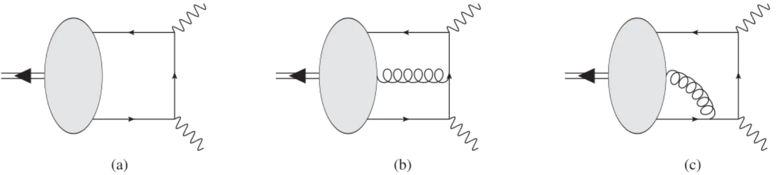
¼ie2ϵμναβqα1qβ2Fπγγðq21; q22Þ; ð1Þ whereeis the electric charge andp¼q1þq2 is the pion momentum. The form factorFπγγðq21; q22Þcan be measured experimentally, at least in principle. If at least one of the photon virtualities is large, the form factor can also be calcu- lated in QCD in terms of a single nonperturbative function describing the quark momentum fraction distributionuin the pion at small transverse separation, the pion DA. For the heuristic discussion in this section, we consider the leading contribution shown in Fig.1; the corrections are discussed in the next section. To this accuracy, one obtains[13]
Fπγγðq21; q22Þ ¼−2 3Fπ
Z 1
0
duϕπðuÞ
uq21þ ð1−uÞq22; ð2Þ whereFπ≃92MeV is the pion decay constant. If the form factor is measured for a wide range of photon virtualities, the pion DA ϕπðuÞ can be extracted from this relation (up to various higher order correction terms). In practice, such mea- surements are very difficult, and experimental information is only available for kinematical situations where one virtu- ality is large and the second is close to zero[14,15], which is not sufficient to map out the completeu-dependence.
The integralR
d4zof(1)receives contributions from both spacelike and timelike separations. Spacelike correlation functions can readily be accessed in lattice simulations.
However, addressing timelike distances is not at all straightforward. The central observation at the root of the recent development is that timelike contributions are not needed (in the present context) as the complete information on the pion DA in principle is already con- tained in the spacelike correlator.
Indeed, to the same accuracy as above,
h0jT
jμ z
2
jν
−z 2
jπ0ðpÞi
¼ 2iFπ
3π2z4ϵμναβpαzβΦπðp·zÞ; ð3Þ
(a) (b) (c)
FIG. 1. The leading-twist (a) and higher-twist (b), (c) leading order contributions to the pion transition form factor.
where
Φπðp·zÞ ¼ Z 1
0 dueiðu−1=2Þp·zϕπðuÞ ð4Þ is the pion DA in longitudinal position space, which is analogous to the Ioffe-time parton distribution in deep- inelastic lepton-hadron scattering [16,17]. The correlation function in Eq. (3) can be calculated on the lattice for spacelike separations z2<0 and in principle arbitrarily large values of the scalar product p·z. In this way, Φπðp·zÞ can be directly measured[12].
Before going into details, we discuss the structure of the position space DA at a qualitative level to understand what kind of information can be obtained from such a meas- urement. Note that in the limit of exact isospin symmetry the equality ϕπðuÞ ¼ϕπð1−uÞ holds. As a consequence Φπðp·zÞ is a real function,Φπðp·zÞ ¼Φπð−p·zÞ, with the normalization conditionΦπð0Þ ¼1. The second deriva- tive at the origin, Φ00πð0Þ, is related to the first nontrivial moment of ϕπðuÞ, which is usually denoted as hξ2i and referred to as the second Mellin moment in the DA literature,
Φ00πð0Þ ¼−1 4
Z 1
0 duð2u−1Þ2ϕπðuÞ≡−1
4hξ2i; ð5Þ where ξ¼2u−1. This moment can be obtained on the lattice using conventional techniques[18–21]as the matrix element of a local operator that contains two covariant derivatives. Higher derivatives of Φπ at the origin are sensitive to higher moments. It has become standard to write the pion DA as a series expansion in orthogonal (Gegenbauer) polynomials,
ϕπðu;μÞ ¼6uð1−uÞX∞
n¼0
aπnðμÞC3=2n ð2u−1Þ; ð6Þ
where aπ0¼1. Note that to one-loop accuracy the coef- ficients aπnðμÞ do not mix under evolution of the scaleμ. Moments of the DA can be written in terms of the coefficients in the Gegenbauer expansion, e.g.,
hξ2i ¼1 5þ12
35aπ2: ð7Þ The corresponding expansion of the DA in position space is in terms of Bessel functions (conformal partial waves[12])
Φπðp·z;μÞ ¼X∞
n¼0
aπnðμÞFnðp·z=2Þ; ð8Þ
where
FnðρÞ ¼3 4in ffiffiffiffiffiffi
p2π
ðnþ1Þðnþ2Þρ−32Jnþ3
2ðρÞ: ð9Þ
The first few conformal partial wavesFnðp·z=2Þ,n¼0, 2, 4, are shown in Fig.2. SinceFnðρÞ∼ρn forρ→0, the sum in(8)for fixedp·zis converging very rapidly; only the first few Gegenbauer moments give a sizeable con- tribution. Conversely, this means that, aiming to extract the information on the pion DA beyond the first few moments, one has to include measurements at largep·z[12].
To view this from a somewhat different perspective, consider, for illustrative purposes, the one-parameter class of models
ϕðαÞπ ðuÞ ¼Γð2ðαþ1ÞÞ
Γðαþ1Þ2 ½uð1−uÞα; ð10Þ at the reference scale μ0¼2GeV. Three particular choices,
ϕð1Þπ ðuÞ ¼6uð1−uÞ;
ϕð1=2Þπ ðuÞ ¼8 π
ffiffiffiffiffiffiffiffiffiffiffiffiffiffiffiffiffi uð1−uÞ
p ;
ϕð0Þπ ðuÞ ¼1; ð11Þ
cover a wide range of shapes that appear to be phenom- enologically acceptable. These longitudinal momentum fraction space DAs and the corresponding position space DAs Φπðp·zÞ are plotted in Fig. 3. The differences between the models increase with p·z. However, as demonstrated in Fig. 2, in the range accessible with present-day lattice calculations (jp·zj≲5), the differences are almost entirely due to the variation of the second Gegenbauer moment: aπ2ðμ0Þ ¼0.389, 0.146, 0 for the three above models, respectively.
So far, we have discussed the situation at tree level.
Taking into account QCD corrections, the position space FIG. 2. The first three conformal partial waves (9) in the expansion(8)of the pion DA in position space.
pion DA Φπðp·zÞ in Eq. (3) will be substituted by a function of both scalar invariants,z2andp·z, of the form ΦVVπ ðp·z; z2Þ ¼CVV2 ðp·z; z2; u;μFÞ⊗ϕð2Þπ ðu;μFÞ
þz2CVV4 ðp·z; z2; u;μFÞ⊗ϕð4Þπ ðu;μFÞ
þOðz4Þ; ð12Þ
whereϕð2Þπ ≡ϕπis the twist-2 DA. TheCVVn are coefficient functions that depend at most logarithmically onz2and are calculable in perturbation theory, while μF is the factori- zation scale. We will tacitly assume using dimensional regularization and the modified minimal subtraction (MS) scheme. The superscript VV indicates the dependence of the coefficient functions on the choice of the correlation function used to define the position space DA—two vector currents for the present example, Eq.(3). The leading- (and higher-)twist pion DAs are universal nonperturbative func- tions and independent of this choice. The power-suppressed Oðz2Þ correction terms correspond to higher-twist pion DAs, likeϕð4Þπ . The factorization scaleμFshould be chosen similar in size to2= ffiffiffiffiffiffiffiffi
−z2
p to prevent large logarithms from appearing in the coefficient functions.
The function ΦVVπ ðp·z; z2Þ, and/or similar correlation functions with different choices of currents, can be calcu- lated on the lattice within certain ranges of the two argu- ments. Different strategies have been suggested as to how useful information can be extracted from such lattice data. In this work, we follow the proposal of Ref. [12]
as well as our work [11], carrying out the complete analysis in position space. We keep the distance between the currents sufficiently small to suppress higher-twist effects and to enable the perturbative evaluation of the coefficient functions at the scale μF∼2= ffiffiffiffiffiffiffiffi
−z2
p ≥1GeV, i.e., ffiffiffiffiffiffiffiffi
−z2
p ≲0.4fm. At the same time, ffiffiffiffiffiffiffiffi
−z2
p should be much larger than the lattice spacing, in this work a≈0.071fm, to tame discretization effects.
In the literature, it has also been suggested to carry out a one-dimensional Fourier transformation of the lattice data in order to define new observables that are closer in spirit to the initial DA in longitudinal momentum fraction space, e.g., aquasidistribution[22–33],
ϕquπ ðwÞ∼ Z ∞
0
dλ
2πe−iðw−1=2Þλp·zΦXYπ ðλp·z;λ2z2Þ; ð13Þ or apseudodistribution [34–36],
ϕpsπðwÞ∼ Z ∞
0
dλ
2πe−iðw−1=2Þλp·zΦXYπ ðλp·z; z2Þ: ð14Þ Both expressions are designed in such a way that, to leading-twist accuracy, they reproduce the pion DA at tree level. In the existing calculations which employ the above methods, two spatially separated quark fields are connected with a Wilson line. Equivalently, this construction can be viewed as a correlation function involving two bilinear currents with an auxiliary “heavy” quark field [37–39]
rather than the light quark field we use in Eq.(3). Apart from employing a Wilson line[22–36,40]or an auxiliary light quark propagator [11,12,41], other obvious choices for connecting the two positions include a scalar propagator [7,8]or a heavy quark propagator[42] or just employing Coulomb gauge[43].
Another technical difference of the quasidistribution work relative to our approach is the use of the large- momentum factorization scheme at an intermediate step (large momentum effective theory [44,45]) to emphasize that, for a large pion momentum and at a fixed quark momentum fraction, large-distance (i.e., higher-twist) con- tributions are suppressed.
III. QCD FACTORIZATION A. Collinear factorization in position space A general approach to implement collinear factorization of QCD amplitudes in position space is provided by the light-ray operator product expansion (OPE)[46–51]. For a generic current product, one writes
FIG. 3. Three models for the pion distribution amplitude(11)in momentum fraction (upper panel) and position space (lower panel). Note thatΦπð−p·zÞ ¼Φπðp·zÞ.
J1ðz1ÞJ2ðz2Þ ¼Z1Z2 Z 1
0 dα Z 1
0 dβC12ðz12;α;β;μFÞ
×Πμl:t:F½qðz¯ ðαÞ12Þ=z12γ5qðzðβÞ21Þ þ ; ð15Þ where
z12¼z1−z2; zðαÞ12 ¼ ð1−αÞz1þαz2; ð16Þ while Zk are the renormalization factors for the currents, Πμl:t:F½… is the leading-twist projection operator, C12 is the coefficient function, and the ellipses stand for higher- twist contributions. For simplicity, we disregard the flavor structure, showing only the contribution of flavor- nonsinglet axial-vector operators that will be important for this work. The corresponding expression for the product of quark and antiquark fields connected by a Wilson line is exactly the same, withZ1,Z2substituted by the quark field renormalization factors in spacelike axial gauge.
The leading-twist projection of a nonlocal quark- antiquark operator is defined as the generating function ofrenormalizedlocal leading-twist operators (traceless and symmetrized over all indices), e.g.,
Πμl:t:F½qðz¯ 1Þ=z12γ5qðz2Þ
¼X∞
n¼1
Xn−1
k¼0
zμ121…zμ12nð−1Þk
2n−1k!ðn−k−1Þ!On;kμ1…μnðzÞ; ð17Þ where z¼ ðz1þz2Þ=2and
On;kμ1…μnðzÞ ¼qðzÞγ¯ ðμ1D⃖ μ2…D⃖ μkþ1D⃗ μkþ2…D⃗ μnÞγ5qðzÞ: ð18Þ Here and below, we indicate trace subtraction and sym- metrization by enclosing the involved Lorentz indices in parentheses, e.g.,OðμνÞ ¼12ðOμνþOνμÞ−14gμνOλλ.
The light-ray OPE differs from the usual Wilson expan- sion in local operators by imposing a different power counting. In the latter case, one assumes that the distance between the currents is small, jz12j∼ηΛ−1QCD withη→0, and the operator matrix elements are of order unity in this limit,hOn;kμ1…μni∼ΛnQCD. In this case, only a finite number of local operators on the r.h.s. of Eq.(17)has to be kept, and also the higher-twist operators must be added pro- gressing to higher powers of η: The relevant expansion parameter is the operator dimension, not the twist. The light-ray OPE assumes instead thathOn;kμ1…μni∼η−nΛnQCDso thatzμ121…zμ12nhOn;kμ1…μni ¼Oð1Þ, and in this case, the series (17) must be resummed to all orders. Such a situation occurs if the hadron has large momentum, jpj ¼Oðη−1Þ and hence p·z12¼Oð1Þ, since for generic hadronic matrix elements
hH0ðpÞjOn;kμ1…μnjHðpÞi∼pðμ1…pμnÞhhOn;kii; ð19Þ
where the reduced matrix element ⟪On;k⟫¼Oð1Þ.
Higher-twist operators of the same dimension have smaller spin (by definition). As a consequence, their matrix elements involve lower powers of the large momentum and are suppressed. At the amplitude level, expanding in powers of the large momentum corresponds to the classi- fication in terms of the so-called collinear twist; see, e.g., Refs.[51,52].
Note that the above power counting is applicable both in Minkowski and Euclidean space. In Minkowski space, one can employ a reference frame where all components of the momentum are small and simultaneously the separation between the currents is almost lightlike, jzμj ¼Oð1Þ, z2¼Oðη2Þ→0. In this way, the usual interpretation as the light-cone expansion arises.
The light-ray OPE provides a technique to deal with leading-twist projected operators(17)as a whole, avoiding the local expansion. These can be viewed as analytic operator functions of the separation between the currents (all short-distance and light-cone singularities are sub- tracted) and satisfy the equation[48]
□z12Πμl:t:F½qðz¯ 1Þ=z12γ5qðz2Þ ¼0: ð20Þ Explicit expressions for the projection operatorΠμl:t:F can be found in Refs.[48,51–53]. This technique combined with the background field method has proven to be very efficient and has found many applications, e.g., in light-cone sum rules[54]for the calculation of higher-twist contributions and for the derivation of the evolution equations for off- forward parton distributions[55,56].
Hadronic matrix elements of the operator (17) define leading-twist parton distributions. Specializing to our case, the pion DA is defined via
h0jΠμl:t:F
¯ q
z 2
=zγ5q
−z 2
jπ0ðpÞi
¼iFπ Z 1
0 duΠl:t:½ðp·zÞeiðu−1=2Þp·zϕπðu;μFÞ; ð21Þ where[50]
Πl:t:½ðp·zÞeiðu−1=2Þp·z
¼
ðp·zÞ−i
8ð2u−1Þm2πz2
eiðu−1=2Þp·zþOðz4Þ: ð22Þ The second term in the last line is the (twist-4) pion mass correction, which is analogous to the Nachtmann target mass correction in deep-inelastic scattering.
B. Choice of currents and one-loop results In this work, we perform a lattice study of the set of correlation functions
TXYðp·z; z2Þ ¼ h0jJ†X z
2
JY
−z 2
jπ0ðpÞi; ð23Þ where the currentsJX≡q¯ΓXuare defined as
JS¼qu;¯ JP¼q¯γ5u;
JμV¼q¯γμu≡JVμ; JμA¼q¯γμγ5u≡JAμ ð24Þ and contain an up quarkuand an auxiliary quark fieldq. In this study, we assume that the auxiliary quark has different flavor than (q≠u,d), but the same mass (mq¼mu) as the light quarks. For convenience and better readability, we invoke the obvious notationTμνVA≡TVμAν, etc.
We do not consider the correlation functions of S(P) with V(A) currents because they are dominated by (chiral odd) higher-twist DAs. For the correlators with two Lorentz indices, the most general invariant decomposition reads TμνVV¼iεμνρσpρzσ
p·z TVV; TμνAA¼iεμνρσpρzσ
p·z TAA; ð25aÞ TμνVA¼pμzνþzμpν−gμνp·z
p·z Tð1ÞVAþpμzν−zμpν p·z Tð2ÞVA þ2zμzν−gμνz2
z2 Tð3ÞVAþ2pμpν−gμνp2 p2 Tð4ÞVA
þgμνTð5ÞVA; ð25bÞ
where the prefactors are by construction invariant under rescaling of z and all invariant functions TXY≡ TXYðp·z; z2Þhave the same mass dimension. The Lorentz decomposition forTμνAVis obtained from the one forTμνVAby
replacing V↔A. One can show that TVA≡Tð1ÞVA is the only invariant function in the VA correlator that receives contributions from the leading-twist DA at leading order in perturbation theory, so that we only consider this structure in what follows. The projection needed to isolate it is specified in AppendixA. Finally, TSP and TPS are scalar functions which we write below as TSP and TPS, respec- tively, to unify the notation.
Separating a common overall prefactor, it is convenient to write the correlation functions in the form
TXYðp·z; z2Þ ¼Fπ p·z
2π2z4ΦXYπ ðp·z; z2Þ; ð26Þ where to tree-level accuracy and neglecting higher-twist correctionsΦXYπ ðp·z; z2Þ ¼Φπðp·zÞis the position space pion DA of Eq.(4). We further separate the leading-twist (LT) contribution from the higher-twist (HT) part, ΦXYπ ðp·z; z2Þ ¼ΦXYπ;LTðp·z; z2Þ þΦXYπ;HTðp·z; z2Þ; ð27Þ where the higher-twist contributions are of Oðz2Þ, cf. Eq.(12). The calculation of the one-loop, i.e., OðαsÞ, correction at leading twist is relatively straightforward.
Using the Gegenbauer expansion of the pion DA, Eqs.(6) and(8), the result can be written as
ΦXYπ;LT¼X∞
n¼0
HXYn ðp·z;μÞaπnðμÞ: ð28Þ Setting the renormalization and factorization scales to the same valueμ¼μF, we obtain, toOðαsÞaccuracy,
HSPn ¼HPSn ¼
1þαsCF
4π ð7η−11Þ
FnðρÞ−αsCF π
Z1
0
dsFnðsρÞ
ðη−4Þsinð¯sρÞ 2ρ þ
ðη−2Þs
¯
sþlnð¯sÞ
¯ s
þcosð¯sρÞ
; ð29aÞ
HVAn ¼HAVn ¼
1þαsCF 4π ðη−5Þ
FnðρÞ−αsCF π
Z1
0
dsFnðsρÞ
ðη−2Þsinð¯sρÞ 2ρ þ
η−1
2 s
¯ sþlnð¯sÞ
¯ s
þ−1 2
cosð¯sρÞ
; ð29bÞ
HVVn ¼HAAn ¼
1þαsCF 4π ðη−5Þ
FnðρÞ−αsCF π
Z1
0
dsFnðsρÞ
ðη−2Þsinð¯sρÞ 2ρ þ
η−1
2 s
¯
sþlnð¯sÞ
¯ s
þcosð¯sρÞ
; ð29cÞ whereαs¼αsðμÞ, the functionsFn are defined in Eq.(9),ρ¼p·z=2,CF ¼43,η¼1þ2γEþlnð−z2μ2=4Þ,s¯¼1−s.
In the following, we will chooseμ≡2= ffiffiffiffiffiffiffiffi
−z2
p . The plus prescription is defined as usual:
Z 1
0 dsfðsÞ½gðsÞþ≡ Z 1
0 ds½fðsÞ−fð1ÞgðsÞ: ð30Þ The sum in (28)converges very rapidly since
FnðρÞρ→0≃ 3 8in
ρ 2
n ffiffiffi pπ
ðnþ1Þðnþ2Þ
Γðnþ5=2Þ ; ð31Þ cf. Fig. 2, so that for moderate p·z only the first few Gegenbauer moments give a sizeable contribution [12].
The two-loop corrections Oðα2sÞ are known for the VV correlator[12]but not for other cases, so we do not include them in this study.
The leading Oðz2Þ higher-twist contribution can be estimated using models for the twist-4 pion DAs derived in Refs.[57,58]; see also Appendix B. One obtains
ΦXYπ;HT¼z2 4
Z1
0
ducos
u−1 2
p·z
fXYðuÞ þOðz4Þ;
ð32Þ where
fSP ¼ ðfPSÞ¼−20δπ2u2u¯2þm2πuu¯þm2π
2 u2u¯2½14uu¯−5þ6aπ2ð3−10uuÞ þ¯ im2π
2ðp·zÞ; ð33aÞ
fVA¼fAV¼−20
3 δπ2uuð1¯ −6uuÞ þ¯ m2π
12uuð19¯ −18aπ2Þ þm2π
2 u2u¯2½7uu¯−8þ18aπ2ð2−5uuÞ;¯ ð33bÞ fVV¼80
3 δπ2u2u¯2þm2π
12u2u¯2½42uu¯−13þ18aπ2ð7−30uuÞ;¯ ð33cÞ fAA¼80
3 δπ2u2u¯2þm2π
12u2u¯2½42uu¯−13þ18aπ2ð7−30u¯uÞ þ2m2πu¯u: ð33dÞ
The parameterδπ2 is defined in Eq. (B10). QCD sum rule estimates yield δπ2≃0.2GeV2 at the scale μ¼1GeV [57–59]. In comparison, theOðm2πÞterms are rather small.
For reasons that will be explained in Sec. IV B, we choose to analyze linear combinations of correlation functions, PSþSP, VAþAV, and VVþAA, to which the leading quark mass correction originating from the chiral odd part of the auxiliary quark propagator does not contribute. In this sum, e.g., the imaginary parts of the SP and PS correlators cancel each other and drop out. For the VAþAV case, the terms linear in the quark massmq drop out completely after applying the projection onto the invariant function of interest as described in AppendixA.
Note that the entire difference betweenfVVandfAAis due to this quark mass correction, which is converted into an Oðm2πÞ term using the axial Ward identity andmq ¼mu.
As observed already in Ref. [12], the higher-twist correction in the VV channel has opposite sign compared to the leading-twist term. We find a similar behavior for the AV channel. In contrast, the twist-4 correction for the SP correlation function has the same sign as the leading-twist contribution. Numerically, the higher-twist corrections turn out to be approximately the same size as the leading perturbative correction at ffiffiffiffiffiffiffiffi
−z2
p =2∼0.2fm≃1GeV−1 and become gradually less important for smaller distances.
At the lowest scale considered in this study, 1 GeV, and at p·z¼0, the combined one-loop and higher-twist
correction yields approximately−40%,−20%, andþ50%
for the VV, VA, and SP channels, respectively. We will find that these estimates are strongly supported by our lattice data, cf. Sec.V.
IV. LATTICE CALCULATION
We employ the same gauge ensemble as in Ref. [11]
(ensemble IV of Ref.[60], generated by the QCDSF and RQCD collaborations), which allows a direct comparison between the sequential source method [61] (used in Ref.[11]) and the stochastic method (applied in this work) for the scalar-pseudoscalar channel. We employ the Wilson gluon action with two mass-degenerate flavors of non- perturbatively order a improved Sheikholeslami-Wohlert [62](i.e., clover) Wilson fermions. The lattice consists of 323×64 points with periodic boundary conditions (anti- periodic in time for the fermion fields). The inverse gauge coupling parameter reads β¼5.29, and the hopping parameter value is κ¼0.13632. This corresponds to the lattice spacing a≈0.071fm¼ ð2.76GeVÞ−1 [63] and a pion mass mπ¼0.10675ð59Þ=a≈295MeV [64]. To reduce autocorrelations, we have used a bin size Nbin¼ 20for theNconf ¼2000configurations we have analyzed, cf. Table I. In order to improve the overlap between the interpolating current at the source and the pion state at large momentum, we employ the momentum smearing technique
of Ref.[65](see also Ref.[21]) with APE-smeared spatial gauge links [66].
The operator renormalization is performed as described in Ref. [67]: The renormalization factors are calculated nonperturbatively within the RI0-MOM scheme [68,69]
(along with a subtraction of lattice artifacts in one-loop lattice perturbation theory). These are then converted to the MS scheme using three-loop (continuum) perturbation theory. The corresponding factors for the MS scale μ¼ 2GeV can be found in Table III of Ref. [64]. To be consistent, we employ theNf ¼2specific running ofαsin all perturbative calculations. To this end, we combine the results of Refs. [63,70] to obtain a value of αs at 1000=a≈2.76TeV. From there, we evolve it downward using five-loop running[71]. The pseudoscalar and scalar currents are evolved to other scales using the four-loop mass anomalous dimension, which is consistent with the order used in Ref.[67]. The numerical values of theNf¼2 coefficients are summarized, e.g., in Ref.[72], which also includes the five-loop calculation.
Disconnected quark line diagrams have proven to be notoriously challenging in lattice simulations. They can be avoided by implementing an appropriate flavor structure of our currents: we pretend that the auxiliary quark fieldqof Eq.(23)is of a different flavor but shares its mass with the light quarks: mq¼mu¼md. This does not present any limitation as the perturbative matching is carried out using the same conventions.
In the following sections, we use boldface letters for the space components of the distance and momentum,ðzμÞ ¼ ð0;zÞandðpμÞ ¼ ðEp;pÞ. In the actual lattice calculation, we evaluate the three-point functions using currents posi- tioned at z, relative to our origin 0. These are “shifted” afterward to the symmetric locations as in Eq. (23) by multiplication with the appropriate phase.
A. Stochastic estimation of correlation functions We wish to compute the correlation functions, Eq.(23).
The corresponding three-point functions for different Γ structures are depicted in Fig. 4, where the straight lines correspond to quark propagators. The momentum- smeared, momentum-projected pion source is located at the Euclidean time slice 0. Translational invariance of the correlation function implies thatzand0can be shifted to the positionsz=2and−z=2, respectively, by multiplication with the phase eip·z=2. Previously, in Ref. [11], we com- puted propagators, starting from a point source at the positionðt;0Þ, smeared the resulting propagator at the time slicet¼0and computed a sequential propagator[61]from there. This propagator and the original propagator were then contracted with theΓX structure atðt;zÞ, making use ofγ5-Hermiticity of the propagatorG, i.e.,Gxy¼γ5G†yxγ5. In order to increase the statistics, ideally one would average over different spatial positionsyof the currentJY,
placingJXat positionsyþz, keeping the relative distance vector fixed. It turns out that this is indeed possible, introducing stochastic propagators[73], albeit at the cost of additional (but small) stochastic noise.
Therefore, our new approach is to start from a momen- tum-smeared pion source att¼tsrcand compute stochastic forward propagators from there, using the“one-end trick” [74]. As with the sequential method adopted by us previously, the external momentum is fixed at the source.
Since we need to keep the distance z between the local currents JX and JY at the sink fixed, volume averaging would not be possible if we created a sequential propagator at the sink. Instead, we use a second stochastic volume source at tsink to connect these two currents. In order to reduce the associated stochastic noise, we utilize the hopping parameter expansion in the way suggested in Refs. [75,76](see also Refs. [77,78]for related work) to block out the dominant short-distance noise contributions when connecting the two currents with a stochastic propagator. Below, we describe our implementation in detail.
We define the momentum smearing operatorFp ¼ΦnðζpÞ with n smearing iterations (n¼200 in our calculation).
This is diagonal in spin and constructed on the time slice tsrc, iteratively applying the operation
ðΦðkÞqÞx ¼ 1 1þ6ε
qxþεX3
j¼1
Ux;je−ik·ˆjqxþaˆj
; ð34Þ
where Ux;j is an APE-smeared [66] spatial gauge link connecting the lattice pointsðtsrc;xÞandðtsrc;xþaˆjÞ; for details, see Refs. [21,65]. In practice, this smearing is implemented by multiplying the spatial connectors within the time slice in question by the appropriate phases,
FIG. 4. The relevant triangle diagram, with a smeared inter- polating current for the pion at t¼0. The Fourier transform corresponds to an incoming pion with momentump(fort >0) or an outgoing pion with momentum−p(ift <0).
Ux;j↦e−iakjUx;j, where k¼ζp. We choose ζ¼0.8 andϵ¼0.25.
We write the Wilson-Dirac operator as
D¼ 1
2aκð1−HÞ: ð35Þ We also define the time, spin, and color diagonal momen- tum projection operator φp with the components
ðφpÞxy¼e−ip·xδxy: ð36Þ
Note thatFp ¼F†p¼F⊺−pis self-adjoint, whileφp ¼φ⊺p¼ φ†−p and D¼γ5D†γ5 are not. We start from a stochastic Z2⊗iZ2 wall source ξ with ξi;αðt;xÞ¼ ð1iÞ= ffiffiffi
p2 δttsrc, where i and αdenote the color and spin indices, respec- tively. We then solve
aDχ¼F−pφ−pξ; aD˜χ ¼Fpξ; ð37Þ whereχ andχ˜ (as well asξ) are Dirac vectors with color, spin, and spacetime components. Above, we have sup- pressed these indices for enhanced readability. In our conventions ξ, χ, and χ˜ (as well as η and s, which will be introduced below) are dimensionless.
We define a momentum-smeared interpolator that, when applied to the vacuum, will create states with the quantum numbers of aπ0carrying the (spatial) momentum p,
O†pðtÞ ¼a3X
x
eip·xO†πðxÞ;
O†πðxÞ ¼ ½uF¯ −pxγ5½Fpux−ðu→dÞ; ð38Þ and a local isovector currentJv¼ ð¯uΓu−d¯ΓdÞ=2with an arbitrary Dirac structureΓ. In the following, we assume, for the sake of readability, that all sources have been shifted to tsrc¼0(exploiting translational invariance) and denote the source-sink distance as t. We can now obtain the average over the spatial volume V3 of smeared-local two-point functions
Cðp; tÞ ¼ h0jJvðt;0ÞO†pð0Þj0i
¼ a6 V3
X
x;y
eip·ðx−yÞh0jJvðt;yÞO†πð0;xÞj0i ð39Þ
as an inner product over color, spin, and (three- dimensional) space:
Cðp; tÞ ¼−a6
2V3htrγ5Fpu⎴0u¯tΓφpu⎴tu¯0F−pφ−pi þ ðu→dÞ
¼ −1
a2V3hðξ;γ5FpD−10tΓφpD−1t0F−pφ−pξÞi
¼−1
V3hð˜χt;φpγ5ΓχtÞi: ð40Þ Here, we have suppressed all unnecessary indices. The disconnected contractions drop out since we have exact isospin symmetry. The minus sign in the first line is due to fermion anticommutation. Within the scalar product ðA; BÞ ¼A†B, we sum over all indices that are not displayed on either side, in this case spatial position, color, and spin. In the second line, we used a−4D−10t ¼ q⎴0q¯t for q∈fu; dg. In the last step, we made use of the orthonormality of the noise vectors when averaged P
XYhξYAYXξXi ¼ hP
XAXXi, whereX,Y represent multi- indices, and of theγ5-Hermiticity of the propagator.
Inserting a complete set of states in Eq. (39) and choosing an axial-vector current at the sink with Γ¼γ0γ5 gives
C2ptðp; tÞ ¼X
n
h0jAv0ð0ÞjnðpÞie−EnðpÞt
2EnðpÞhnðpÞjO†πð0Þj0i
→ZπðpÞe−EπðpÞt
2EπðpÞh0jAv0ð0Þjπ0ðpÞi ðt→∞Þ:
ð41Þ The overlap factor ZπðpÞ ¼ hπ0ðpÞjO†πð0Þj0i depends on the (momentum-smeared) interpolator, while
h0jAvμð0Þjπ0ðpÞi ¼iFπpμ ð42Þ defines the pion decay constant.
To construct the desired three-point function, we use additional spin-partitioned [79] (also referred to as spin explicit or “diluted” in the literature) stochastic sources ηðk;αÞ,k¼1;…; nst, andα¼1;…;4, with the components ηðk;αÞi;βðt;xÞ ¼rðkÞix δαβδttsink. The random variablesrðkÞix take the values ð1iÞ= ffiffiffi
p2
. We then solve
aDsðk;αÞ¼ηðk;αÞ ð43Þ
for each value of k and α to obtain sðk;αÞ. The lattice propagator G¼a−4D−1 fromðt;yÞto ðt;yþzÞcan now be estimated as
Gðt;yþzÞðt;yÞ≈ 1 a3nst
X
k;α
sðk;αÞðt;yþzÞηðk;αÞ†ðt;yÞ ; ð44Þ up to a stochastic error that decreases ∝1= ffiffiffiffiffiffiffiffiffiffiffiffiffiffiffiffi
Nconfnst
p ,
where Nconf is the number of gauge configurations and nst¼10 is the number of spin-partitioned stochastic sources.
The operatorHin Eq.(35)only couples nearest neighbors for the action we use. Employing the geometric series
a3G¼ ðaDÞ−1¼2κð1−HÞ−1¼2κX
j≥0
Hj
¼2κmðzÞ−1X
j¼0
Hjþ2κ X
j≥mðzÞ
Hj
¼2κmðzÞ−1X
j¼0
HjþHmðzÞa3G; ð45Þ where
mðzÞ ¼X3
i¼1
min jzij
a ;L−jzij a
; ð46Þ
we can split up the propagator into the first sum in Eq.(45) that does not contribute at distancesz(and distances that are separated by a larger number of hops) and a part that contributes. In the stochastic estimation, the first part still adds to the noise. This undesirable effect can be removed, left multiplying the solution withHmðzÞ[75,76].
Looping over momenta and times, we define temporary scalar fields
Kðm;k;αÞX ðyÞ ¼χ˜†ðt;yÞγ5ΓXHmsðk;αÞðt;yÞ; ð47Þ Kðk;αÞY ðyÞ ¼e−ip·yηðk;αÞ†ðt;yÞ ΓYχðt;yÞ ð48Þ for m≤10 and all currents of interest. These fields implicitly depend onp andt. Also note that the solutions χandχ˜ of Eq.(37)depend on the momentump. The three- point correlation functions can now readily be obtained by replacing Jvðt;yÞ↦J†Xðt;z=2ÞJYðt;−z=2Þ in Eq. (39) (cf. Fig. 4). The result reads
C3ptXYðp; t;zÞ ¼ −e2ip·z a3V3nst
X
y;k;α
hKðm;k;αÞX ðyþzÞKðk;αÞY ðyÞi;
ð49Þ where the value of m≤mðzÞ used within the set of precomputed fieldsKðm;k;αÞX is selected as large as possible for each distance. Note that we have already shifted the above correlation function to the symmetric position. In our study, we limit ourselves to the range jzij≤5a.
With the previous sequential source method, first one propagator (12 solves) had to be computed. Then, for each additional momentum and time separation, two smearing operations were required as well as an additional propagator (12 solves). In our implementation of the new method, we vary the distance between the pion source and the sink by changing the time slice where the pion source is placed, enabling us to reuse the stochastic
solutions Hmsðk;αÞ and sources ηðk;αÞ of Eqs. (47) and (48). This part requires 4nst ¼40 solves with a minimal overhead from applying the hopping parameter expansion.
For each momentum and time separation, a new pion source is seeded, necessitating only two additional smear- ing operations and two additional solves.
In total, not even taking into account that there is an additional gain from the two possibilities of connecting the valence quark propagators with the stochastic propagator of the auxiliary field (giving us for each momentum p the momentum−palmost for free), the new method does not only allow for a volume average, thereby reducing stat- istical errors, but turns out to be cheaper by about a factor of 2 in terms of the total computer time.
The three-point function C3ptXY admits the same spectral decomposition, Eq. (41), as the two-point function C2pt. Just the matrix element needs to be replaced:
h0jAv0ð0Þjπ0ðpÞi↦h0jJ†Xð0;z=2ÞJYð0;−z=2Þjπ0ðpÞi. The overlap factor ZπðpÞ and the exponential decay cancel when taking the ratio of these two functions. Therefore, in the limit of large Euclidean times, where excited state contributions are exponentially suppressed, the ratio can be related to the matrix element of interest,
TXYðp·z; z2Þ
Fπ ¼ZXðμÞZYðμÞ ZA
C3ptXYðp; t;zÞ
C2ptðp; tÞ iEπðpÞ; ð50Þ whereZXis the renormalization factor of the local current JX with respect to the MS scheme [67]. For the scalar and the pseudoscalar currents, the renormalization fac- tors acquire a scale dependence due to their anomalous dimension.
B. Reducing discretization effects
In the continuum, the chiral even part (∝=z) of the propagator connecting the two local currents gives the most important contribution, while thechiral odd part (∝1) is suppressed by a factorm ffiffiffiffiffiffiffiffi
−z2
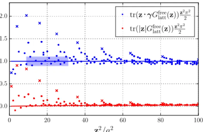
p and, thus, can be set to zero in a first approximation. However, with Wilson fermions, the situation is completely different. We find that the contribution from the chiral odd part, which suppresses the doublers and breaks chiral symmetry, can be of the same order of magnitude as the leading contribution, cf. Fig.5. The“jumping”of the points nicely demonstrates the strong dependence of the lattice artifacts on the chosen direction. In particular, the points along the axes [e.g., (1,0,0)], corresponding to the crosses in Fig.5, exhibit the largest discretization effects, while the points along the diagonal [e.g., (1,1,1)] are much better behaved. This fits in with earlier observations for correlation functions[80–82]
and quark propagators in momentum space[83]. The large contribution of the chiral odd part of the propagator is a peculiarity of using Wilson fermions, while large discre- tization effects at short distances are probably a general feature of all position space methods.
The appearance of large contributions from the chiral odd part of the propagator would lead to huge lattice artifacts in the correlator. Therefore, we construct linear combinations of the correlation functions defined in Eqs.(25)where the chiral odd part of the propagator drops out to leading order in perturbation theory:
1
2ðTSPþTPSÞ; 1
2ðTVAþTAVÞ; 1
2ðTVVþTAAÞ: ð51Þ For the scalar-pseudoscalar correlator with a pion, this is equivalent to taking the real part (cf. Ref. [11]).
The discretization effects in the chiral even part of the propagator (these correspond to the blue points in Fig. 5) are addressed as follows: we discard data points where the free field discretization effect exceeds 10%. This cut mainly excludes very short distances (jzj≲2a) and directions close to the lattice axes. For the remaining data points, we define a correction factorccorrðzÞsuch that the corrected propagator
GcorrlattðzÞ≡ccorrðzÞGlattðzÞ ð52Þ satisfies the condition
trf=zGcorrlattðzÞg ¼! trf=zGcontðzÞg; ð53Þ where the trace runs over spin and color indices. To zeroth order accuracy in αs (where Glatt¼Gfreelatt is the free propagator), this leads to
ccorrðzÞ ¼
trDf=zGfreelattðzÞgz2π2 2
−1
ð−m2z2Þ
2 K2ðm ffiffiffiffiffiffiffiffi
−z2 p Þ:
ð54Þ
This corresponds to multiplying the blue data points of Fig. 5 by factors so that in the noninteracting case the continuum result is retrieved. One should note that this procedure can only tame distance-dependent discretization effects. However, there are also momentum-dependent discretization effects, which are not taken into account.
It is therefore no surprise that we still find particularly large discretization effects for the high momentum data at small distances. We have therefore decided to include only data points withjzj≥3a≈0.21fm, which, setting the scale to μ¼2=jzj, corresponds toμ≲1.84GeV.
Finally, we remark that the pseudoscalar and scalar currents are (up to small mass-dependent effects) auto- matically order a improved. In principle, we could also have order a improved the axialvector and the vector currents. However, the improvement of γμγ5 and of γμ would have required us to compute three-point functions with two currents situated at nonequal times (as well as a tensor current in the latter case).
V. RESULTS
A. Parameter choices and first data survey Our analysis includes six different pion momenta (12, if one counts p separately) with absolute values up to jpj ¼2.03GeV, cf. TableI. For the largest momentum, we have analyzed two different directions to increase statistics.
Reaching such a large hadron momentum is quite chal- lenging and was achieved by the combination of the momentum smearing technique, which enhances the over- lap of the interpolating current with hadrons at large momenta, and the use of stochastic estimators described in Sec.IVA, which allows us to take a volume average at the cost of additional stochastic noise. The latter trade-off turns out to be very advantageous and yields a significant reduction of the statistical errors compared to the sequential source method used in Ref.[11].
Since the lattice data are analyzed using QCD factori- zation in the continuum, we are bound to using sufficiently small separations between the currents to ensure that the coefficient functions are perturbatively calculable.
FIG. 5. The (free field) discretization effects of the Wilson propagator compared to the continuum expectation (full lines) for the different Dirac structures. The points marked with a cross correspond to directions along a lattice axis. The shaded area marks the distances that are actually used in the analysis, where the upper limit comes from the constraintμ¼2=jzj>1GeV. It is clear that smaller lattice spacings will improve the situation considerably.
TABLE I. The lattice momenta used in the analysis, where p¼2πLnp.Nconf is the number of analyzed configurations, and Nbin is the bin size used to reduce autocorrelations. Note that for the smallest momentum we have used only every tenth configuration.
np jpj Nconf Nbin
ð1;0;0Þ 0.54 GeV 200 2
ð2;0;0Þ 1.08 GeV 2000 20
ð2;2;0Þ 1.53 GeV 2000 20
ð2;2;2Þ 1.88 GeV 2000 20
ð3;2;1Þ 2.03 GeV 2000 20
ð2;−1;3Þ 2.03 GeV 2000 20
Together with the requirement of controllable discreti- zation effects (see the previous section), this leaves us with the relatively narrow range of possible distances 0.21fm≲jzj≲0.39fm, or 3a≤jzj≤5.5a in units of
the lattice spacinga≃0.07fm. Since the direction ofzis arbitrary, this constraint still allows for a large data set with ten different values forjzj.
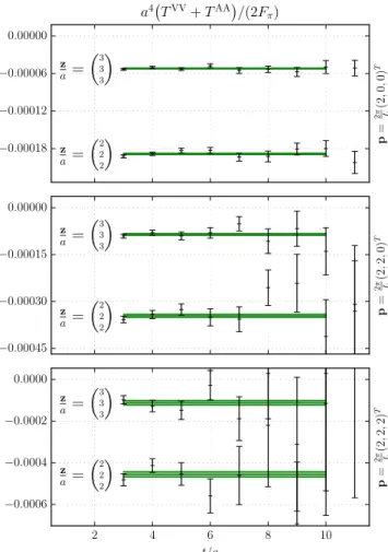
First, however, we should check if the ratios of three-point over two-point functions (50) approach their asymptotic limits. We demonstrate this for the combination ðTVVþ TAAÞ=2 for different momenta and distances in Fig. 6.
Clearly, the momentum smearing was extremely successful in removing excited state contributions. Moreover, these seem to affect the two-point function in a similar way as the three-point functions, enabling additional cancellations to take place. The other channels exhibit a very similar behavior so that we can confidently fit to extended plateaus.
Next, in Fig. 7, we compare our results at two typical distances for two different channels with the expecta- tion obtained using the second Gegenbauer coefficient aπ2ð2GeVÞ ¼0.1364that has been determined in Ref.[20]
with the moment method. The leading-twist position space DA (central solid line) is universal for all channels. The dashed lines include our one-loop perturbative corrections, while the solid lines also include higher-twist effects using the QCD sum rule estimateδπ2ð2GeVÞ¼0.17GeV2 [57–59]. Unsurprisingly, toward the larger distancejzj, both correction terms become more significant. The sign and magnitude of the predicted splitting are in good agreement with our data. However, there are quantitative differences:
our data still show residual discretization effects, the models for the leading-twist and higher-twist DAs may not be correct, and there will be two-loop perturbative corrections as well. For the distances shown, the corrections to the leading order leading-twist DA are about 25% in size, while even at jp·zj ¼4, the differences between the models plotted in Fig. 3 only amount to about 10%; i.e., within our range of z2 andp·z values, we are more sensitive to higher-twist effects and perturbative corrections than we are to the shape of the leading-twist DA. This is also expected from Fig.2and the discussion of Sec.II.
FIG. 6. The ratio (50) for the example of the VVþAA combination of currents for different distances and momenta, together with our fitted results.
FIG. 7. Data for the position space DA at two distances compared with expectations obtained using the second Gegenbauer coefficient aπ2ð2GeVÞ ¼0.1364 determined in Ref. [20] with the moment method. The central solid curve corresponds to the (channel- independent) tree-level result at leading twist. The dashed lines include one-loop perturbative corrections for the two channels, and the outer solid lines also include higher-twist contributions [obtained using the QCD sum rule estimateδπ2ð2GeVÞ ¼0.17GeV2for the higher-twist normalization constant]. The upper data (green) are SPþPS, and the lower data (blue) are VVþAA.
The data points in Fig.7as well as in Figs.8–10below are obtained by performing a weighted average over all possible combinations of the distancez¼ ðz1; z2; z3Þand momentump¼ ðp1; p2; p3Þthat give the same values for
FIG. 9. The same as in Fig.8, but for the VVþAA correlation function.
FIG. 8. The SPþPS correlator as a function ofp·zfor four different separations between the currents. The turquoise, orange, and red bands correspond to fits using the parametrizations A, B, and C explained in the text, cf. Table II. The dashed lines are obtained by subtracting the higher-twist contributions from the parametrizations.