the South Pacific Subtropical Gyre and the Labrador Sea

(1)

The Nature and Variability of Eddy Kinetic Energy

in an Ocean General Circulation Model

With a Focus on

the South Pacific Subtropical Gyre and the Labrador Sea

Dissertation

zur Erlangung des Doktorgrades

der Mathematisch-Naturwissenschaftlichen Fakultät der Christian-Albrechts-Universität zu Kiel

vorgelegt von

Jan Klaus Rieck

Kiel, 2019

(2)

Koreferent: Prof. Dr. Peter Brandt

Tag der mündlichen Prüfung: 05.03.2019

Zum Druck genehmigt: 05.03.2019

gez. Prof. Dr. Frank Kempken, Dekan

(3)

Abstract

This thesis focuses on the nature of oceanic Eddy Kinetic Energy (EKE), its generation and temporal variability. For case studies, two regions of the world’s oceans are se- lected based on their importance for the global ocean circulation, the local occurrence of mesoscale variability, and the level of atmospherically driven oceanic variations.

The first region is located in the subtropical gyre in the South Pacific, and the second region is focused on the Labrador Sea (LS) in the western subpolar North Atlantic. An Ocean General Circulation Model (OGCM) based on the NEMO code builds the foun- dation for these investigations. The model’s ability to simulate the oceanic mesoscale in a configuration with 1/4^◦ horizontal resolution is tested by reducing the horizontal diffusion of momentum. The reduction substantially improves the representation of EKE and its variations in the South Pacific subtropical gyre without exhibiting excessive amounts of grid-scale numerical noise.

For a first case study, several simulations of the 1/4^◦ configuration with varying atmospheric forcing are used to investigate the temporal variability of EKE in the South Pacific Subtropical Countercurrent (STCC). Decadal changes in wind stress curl associated with positive (negative) phases of the Interdecadal Pacific Oscillation (IPO) lead to upwelling (downwelling) south of the STCC and downwelling (upwelling) in the STCC, strengthening (weakening) the meridional density gradient and thereby increasing (decreasing) STCC strength, baroclinic instability and the resulting EKE. An additional 30 to 40%of the local density anomalies can be explained by long baroclinic Rossby waves propagating into the region, modulating the decadal signal of the IPO’s influence in the STCC on interannual time scales.

In a second case study, the model’s horizontal resolution is regionally increased to 1/20^◦ in the North Atlantic to investigate different types of mesoscale eddies in the Labrador Sea. Irminger Rings (IR), Convective Eddies (CE) and Boundary Current Eddies (BCE), their generation mechanisms, and their impact on the central LS are successfully simulated. On decadal time scales, the temporal variability of EKE in the LS is driven by the large-scale atmospheric circulation. In the case of CE, local winter heat loss leads to deep convection, a baroclinically unstable rim-current is established along the edge of the convection area and generates EKE at mid-depth. The variations of EKE associated with the surface intensified IR and BCE are driven by the large-scale changes of the currents of the subpolar gyre. While IR play a vital role in stratifying large parts of the LS and thus suppressing deep convection, CE are the major driver of rapid restratification during and after deep convection.

Overall, the thesis shows that, with a suitable choice of parameters, the OGCM offers the required temporal and spatial resolution and extent to investigate the long-term variations of the mesoscale beyond intrinsic time scales, successfully simulating EKE, its generation, impacts and temporal variability.

(4)

(5)

Zusammenfassung

Diese Arbeit untersucht die kinetische Energie von mesoskaligen, ozeanischen Strö- mungen (EKE), ihre Entstehung, und zeitliche Variabilität. Basierend auf ihrer Re- levanz für die globale Ozeanzirkulation, das lokale Auftreten von mesoskaliger Varia- bilität, und der Stärke von atmosphärisch angetriebenen Veränderungen im Ozean werden zwei Regionen der ausgewählt. Eine Region liegt im subtropischen Wirbel im Südpazifik, die zweite in der Labradorsee (LS) im westlichen subpolaren Nordatlantik.

Ein Ozeanzirkulationsmodell basierend auf dem NEMO-Code bildet den Grundstein für die Studie. Die Fähigkeit des Modells die ozeanische Mesoskala in einer Konfigura- tion mit 1/4^◦ horizontaler Auflösung zu simulieren wird durch eine Reduktion der ho- rizontalen Diffusion von Momentum überprüft. Die Reduktion verbessert die Darstel- lung der EKE und ihrer Veränderungen im südpazifischen subtropischen Wirbel, ohne dabei übermäßig viel numerisches Rauschen auf der Gitterskala zu produzieren.

Für eine erste Fallstudie werden verschiedene Simulationen der 1/4^◦-Konfiguration mit unterschiedlichem atmosphärischem Antrieb genutzt, um die zeitliche Variabi- lität der EKE im südpazifischen subtropischen Gegenstrom (STCC) zu untersuchen.

Dekadische Schwankungen der Rotation der Windschubspannung, hervorgerufen durch positive (negative) Phasen der Interdekadischen Pazifischen Oszillation (IPO), führen zu Auftrieb (Absinken) südlich des STCC und Absinken (Auftrieb) im STCC und einer Stärkung (Abschwächung) des meridionalen Dichtegradienten. Dadurch erhöhen (reduzieren) sie die Stärke des STCC, barokline Instabilität, und die resultierende EKE. Zusätzlich können 30 bis 40%der lokalen Dichteanomalien durch lange, barokline Rossbywellen erklärt werden, die in der Region eintreffen und das dekadische Signal des Einflusses der IPO auf interannualen Zeitskalen modulieren.

In einer zweiten Fallstudie wird die horizontale Auflösung des Modells im Nordatlantik auf 1/20^◦ erhöht um die verschiedenen Arten von mesoskaligen Strömungswirbeln in der Labradorsee zu untersuchen. Irminger Ringe (IR), Konvektive Wirbel (CE) und Randstromwirbel (BCE), ihre Entstehungsmechanismen und ihr Einfluss auf die zen- trale LS werden erfolgreich simuliert. Auf dekadischen Zeitskalen wird die zeitliche Variabilität der EKE in der LS von der großskaligen Zirkulation der Atmosphäre angetrieben. Im Falle der CE führt lokaler Wärmeverlust im Winter zu Tiefenkon- vektion, eine baroklin instabile Strömung entlang des Randes der Konvektionsregion entsteht und produziert EKE in mittleren Tiefen. Die Veränderungen der EKE, die den oberflächenintensivierten IR und BCE zuzuordnen ist, werden durch großskalige Schwankungen der Strömungen im subpolaren Wirbel verursacht. Während die IR eine essentielle Rolle in der Stärkung der Schichtung von großen Teilen der LS spielen und somit die Tiefenkonvektion erschweren, sind die CE der hauptsächliche Grund für die schnelle Wiederherstellung der Schichtung während und nach der Tiefenkonvektion.

Insgesamt zeigt diese Arbeit, dass das Ozeanzirkulationsmodell in Verbindung mit einer angemessenen Wahl der Parameter die erforderliche zeitliche und räumliche Auf- lösung und Ausdehnung bietet, um die langzeitlichen Schwankungen der ozeanischen Mesoskala über intrinsische Zeitskalen hinaus zu untersuchen und die EKE, ihre Entstehung, ihren Einfluss und ihre zeitliche Variabilität erfolgreich zu simulieren.

(6)

(7)

Contents

1 Introduction

1.1 The Nature of Eddy Kinetic Energy

Historic descriptions of the oceans’ circulation assumed the flow to be rather laminar.

Currents and their velocities were estimated based on the geostrophic relationship due to the limited availability of direct current measurements. With the introduction of more sophisticated measurement techniques it became clear however, that most regions of the ocean exhibit an abundance of smaller scale circulation features (cf. Fig.

1.1). These mesoscale currents have spatial scales of tens to hundreds of kilometers and temporal scales of weeks to months (Stammer and Böning 1996). While the tra- ditional ship-based observations of temperature, salinity and velocities revealed more and more details of the mesoscale (e.g. MODE Group 1978), it was hardly possible to quantitatively describe its spatial and temporal distribution in all ocean basins. Only the advance of satellite altimetry made it feasible to directly observe and describe the mesoscale in detail on a global scale (Fu 1983; Le Traon and Morrow 2001).

Figure 1.1: Snapshot (5-day mean field) of horizontal current speed at the sea surface in the North Atlantic from a 1/20^◦ Ocean General Circulation Model (VIKING20X). Light blue to white shading in the northern regions indicates sea ice cover. The land surface image is obtained from NASA Earth Observatory (https://visibleearth.nasa.gov/view.php?id=73884).

(10)

Analogously to the observing systems, numerical modeling of the ocean significantly progressed in the second half of the 20th century. Due to improved numerical techniques and increased computational power, ocean simulations could be run at higher resolutions, effectively simulating the mesoscale (Holland and Lin 1975; Cox 1985;

Smith et al. 2000). Until today, numerical models remain the most important tool to study the oceanic mesoscale. The information gleaned from satellite-borne observing techniques is limited to the ocean surface and although the number of observing platforms in the water column, ship-based and autonomous, has drastically increased, synoptic pictures of whole ocean basins are impossible to obtain at depth. This gap of knowledge is tried to be filled with the help of ocean general circulation models (OGCMs) in configurations that aim at simulating the oceans’ circulation as realisti- cally as possible. High resolution simulations (e.g. von Storch et al. 2012) and theoretical interpretations of observations (e.g. Scott and Wang 2005) reveal that baroclinic instability is the major generation mechanism of mesoscale variability. Baroclinic instability emerges when the horizontal density gradients in the ocean are large, thereby creating strong vertical gradients of the horizontal velocities through the thermal wind relation. The flow becomes unstable and a lateral exchange of properties reduces the horizontal gradients of density, essentially transferring energy from the reservoir of Available Potential Energy to Eddy Kinetic Energy (EKE). Another contribution to the generation of mesoscale currents, especially in strong large-scale current systems, is made by barotropic instability (e.g. Yang et al. 2017; Schubert et al. 2018) that arises when the horizontal gradients of velocity are large, and transfers kinetic energy from the mean flow (MKE) to the mesoscale EKE.

As the generation of mesoscale currents is closely associated with the transfer of energy to the reservoir of Eddy Kinetic Energy, EKE is the most commonly investigated property to study the temporal and spatial distributions of the oceanic mesoscale. Eddy Kinetic Energy describes the velocity manifestations of different mesoscale phenomena such as filamenting and meandering of currents and various forms of vortices and current rings. In general, EKE is large in the vicinity of strong currents such as the western boundary currents or the Antarctic Circumpolar Current, where the velocity gradients are strong (Scharffenberg and Stammer 2010; Xu et al. 2011). Nevertheless, EKE is present in all regions, as baroclinic instability can emerge from relatively weak velocity gradients (Beckmann et al. 1994; Arbic 2000; Spall 2000) and EKE in the form of waves or eddies propagates from its location of generation and could thus reach areas where instabilities are weak or not present (Fu 2009). In the vertical, EKE is most

(11)

1.1 The Nature of Eddy Kinetic Energy

often surface intensified, reflecting the dominance of the first baroclinic mode in wide areas of the ocean (Wunsch 1997). However, there are various instances where EKE has a maximum at depth, such as in Mode Water eddies (e.g. Schütte et al. 2016), Deep Western Boundary Current eddies (Dengler et al. 2004) or Convective Eddies (Lilly et al. 2003).

Studies of mesoscale variability and EKE not only help to dynamically understand how water flows in the ocean. Mesoscale eddies and EKE in general do also impact larger scale hydrographic and dynamic properties and are important for the whole climate system and its changes (Delworth et al. 2012; Kirtman et al. 2012). Kinetic energy is fed back to the reservoir of MKE from EKE, strengthening currents and jets (Berloff et al. 2009; Radko 2016). Additionally, eddies effectively flatten isopycnal slopes due to their down-gradient flux of buoyancy (e.g. Gent and Mcwilliams 1990).

Thus, EKE directly (dynamically) and indirectly (through changes of hydrographic properties) influences the location and strength of currents and fronts. The mean circulation and the associated distribution of sea surface temperature then is a crucial driver of atmospheric circulation, especially atmospheric convection and thus precipitation (Minobe et al. 2008; Frankignoul et al. 2011). Mesoscale features are also known to locally influence atmospheric winds, clouds and precipitation (Frenger et al. 2013;

Small et al. 2014). The distribution and temporal variability of EKE is thus crucial to understand the whole climate system and its potential future changes.

In an ocean-only model, such as the one used in this thesis, an impact of EKE on the atmosphere is not simulated, as the atmospheric state is a prescribed boundary condition. While this inhibits an investigation of the whole feedback loop between atmosphere and ocean, it constitutes a simplified framework in which the influence of the atmospheric variability on EKE can be studied. One advantage of ocean-only models is the ability to perform hindcast simulations, where the ocean is driven by the observed atmosphere of the last decades and thus changes in the model’s circulation can be compared to observed changes. However, variations of ocean currents, and especially the mesoscale, are not always easily connectible to certain changes in the atmosphere. Recent studies show the temporal variations of the oceanic mesoscale to be largely intrinsic or internal to the ocean (Combes and Di Lorenzo 2007; Penduff et al. 2011; Sérazin et al. 2015; Wilson et al. 2015). Even changes of the mesoscale on interannual to decadal time scales cannot be attributed to a certain large-scale atmospheric forcing in many regions. Thus, the number of areas in which investigations

(12)

of the atmosphere’s influence on variations of EKE is expected to yield significant results is limited, and a need for long model simulations to successfully disentangle intrinsic and atmospherically forced variations arises.

1.2 Modeling the Mesoscale

The modeling of the oceanic mesoscale with OGCMs requires the configurations to have a sufficiently high horizontal resolution. A common measure for the ability of configurations to resolve the mesoscale is the ratio of the local grid cell size to the first baroclinic Rossby radius of deformation (e.g. Chelton 1998; Hallberg 2013). The Rossby radius decreases with increasing latitude and also depends on stratification and the ocean’s depth. For the open-ocean regions studied in this thesis, the latitudinal dependence is the major factor to consider. The developments in ocean modeling of the recent decades make it possible to run high-resolution OGCMs that resolve the Rossby radius with at least 2 grid points at a wide range of latitudes (e.g. Smith et al. 2000; Maltrud and McClean 2005; Sasaki et al. 2008; Deshayes et al. 2013) and are thus capable of resolving mesoscale features. However, these configurations are still computational expensive and especially when the necessity of long simulations is taken into account, it seems desirable to rely on coarser-resolution, eddy-permitting configurations to investigate certain processes. An additional advantage of these less expensive configurations is the possibility to conduct a range of sensitivity studies regarding parameter choices and forcing strategies.

While resolutions of 1/10^◦ and higher are inevitable to simulate the mesoscale at midlatitudes and further poleward, eddy-permitting resolutions resolve, at least partly, the most energetic parts of the mesoscale spectrum in the tropics and subtropics. There, a realistic simulation of mesoscale features is often limited by the parameterized diffusion of momentum. In order to prohibit the accumulation of energy at the grid scale, a viscosity parameterization is implemented that removes this energy and mimics its small-scale dissipation. However, the most common forms of viscosity parameterizations also remove energy from scales close to the grid scale. In eddy-permitting simulations, these affected scales lie within the mesoscale range and the choice of viscosity thus directly affects the EKE by dissipating parts of it. To allow for a free evolution of the resolved dynamical scales, the viscosity parameter should be chosen as small as possible. Reducing the viscosity is known to improve the representation of EKE

(13)

1.3 Case Studies

(Böning et al. 1991) and large scale currents (Jochum et al. 2008) in eddy-permitting configurations. At the same time, the viscosity needs to be large enough to ensure numerical stability and suppress spurious diapycnal mixing (Megann 2018). Several constraints such as the viscous Courant-Friedrichs-Levy criterion (Jochum et al. 2008), the Grid-Reynolds number (Griffies and Hallberg 2000), and the Munk boundary layer (Munk 1950) limit the choice of an adequate viscosity parameter. However, these constraints still leave a range of possible values to explore within the specific configuration at hand and the region under investigation.

1.3 Case Studies

As outlined in section 1.1, EKE is of profound importance to the oceanic circulation and its interaction with the atmosphere. However, the intrinsic variability of the ocean hinders meaningful investigations of the atmospheric influence on the temporal variations of EKE in many parts of the world’s oceans. Thus, the selection of regions to focus on in this thesis is not solely guided by their importance to the large scale ocean circulation and the urge to understand the generation as well as the impact of mesoscale variability, but also by the necessity to identify regions in which an attribu- tion of an atmospheric driver to the temporal variations of the mesoscale is possible.

Two of the regions to fulfill these requirements are introduced in the following.

1.3.1 The South Pacific Subtropical Gyre

The subtropical gyre in the South Pacific is a key region for Mode Water formation (e.g. Sato and Suga 2009; Li 2012; Liu and Wu 2012) and thus an important part of the subtropical cells that connect the subtropical and equatorial latitudes (e.g. Lübbecke et al. 2008; Farneti et al. 2014; Yamanaka et al. 2015). Through this connection, the variability of the subtropical South Pacific is communicated to the tropical circulation system and influences dynamic and hydrographic properties of the equatorial ocean, directly associated with El Niño and the Earth’s climate system.

Formation regions of subtropical Mode Water are often located in the vicinity of the subtropical fronts. In the South Pacific, the meridional density gradient across this front drives a near-surface, eastward current (Merle et al. 1969; Morris et al.

(14)

1996), the Subtropical Countercurrent (STCC). At a mean zonal velocity of roughly 5 cm s⁻¹ (Qiu and Chen 2004), it is located between25^◦ and33^◦S above the westward (−2cm s⁻¹) South Equatorial Current (SEC). The vertical shear of the horizontal velocities between the STCC and the SEC generates baroclinic instability (Qiu and Chen 2004), resulting in elevated mesoscale variability along the STCC. The EKE in the STCC exhibits temporal variability on seasonal to decadal time scales driven by changes in the meridional density gradient across the subtropical front (Travis and Qiu 2017). Due to its close proximity to the Mode Water formation regions, changes in the STCC could potentially impact Mode Water and thus the subtropical cells and the equatorial Pacific, especially when considering that mesoscale eddies are known to influence the formation process of Mode Water (Qiu et al. 2007; Nishikawa et al. 2010).

In contrast to other subtropical gyres, the intrinsic variability of the mesoscale in the South Pacific along the STCC is not dominant compared to the variability that can be attributed to an atmospheric forcing (Sérazin et al. 2015). It is thus possible to connect large scale atmospheric variations to the variability of the ocean circulation and its EKE. In this thesis, the focus is put on long-term, decadal changes, as under- standing the mechanisms of these is crucial to predict how the ocean might respond to atmospheric conditions in a changing climate, and also helps to differentiate between trends induced by climate change and decadal-scale variations of the oceanic circulation.

1.3.2 The Labrador Sea

The Labrador Sea (LS) in the western subpolar North Atlantic is one of the key regions in the global-scale oceanic circulation. Due to large heat loss to the atmosphere in winter and favorable preconditioning in the form of a weak oceanic stratification, deep convection regularly occurs in the LS (e.g. Marshall and Schott 1999). The water mass formed during deep convection, the Labrador Sea Water, is one of the contribu- tors to the lower branch of the Atlantic Meridional Overturning Circulation (AMOC).

The AMOC, together with its temporal variability and connection to the atmosphere, is one of the most intensively studied oceanic phenomena. The relative role of deep convection in the LS in supplying water to the equatorward, deep flow of the AMOC, and also the connections and feedbacks between the AMOC and the atmosphere are highly debated, especially because different observations and simulations lead to dif-

(15)

1.3 Case Studies

ferent interpretations of how the AMOC will behave in a warmer future climate (e.g.

Lozier et al. 2010; Srokosz et al. 2012).

Due to its role in the AMOC, the LS was extensively studied in the past two to three decades, and various studies found mesoscale, oceanic eddies to play a major role in determining both the location and strength of deep winter convection and the subsequent restratification of the convected water mass during spring and summer.

Different types of eddies can be distinguished in the LS based on their origin, properties, vertical structure and size. The warm-core, anticyclonic Irminger Rings (IR) have diameters of 30-60 km (Lilly et al. 2003; Brandt et al. 2004) and propagate west and southwest (Katsman et al. 2004; Zhang and Yan 2018) from the West Greenland Current (WGC). In the northern central LS, they play a substantial role in stratifying the water column, thus suppressing deep convection (Chanut et al. 2008). Their role in restratifying the southern central LS (the area of observed deep convection), as well as their generation mechanisms are still debated. Additionally, smaller eddies with maximum velocities at mid-depth are found in the central LS around the edge of the convection area (Gascard and Clarke 1983; Send et al. 1995; Lilly et al. 2003). These so-called Convective Eddies (CE) are thought to effectively exchange water between within and outside the mixed patch, resulting in a restratification of the central LS.

Another class of small eddies is the Boundary Current Eddies (BCE). In contrast to CE, they are shallow, surface-intensified and originate from the boundary currents along the shelf of the LS.

The EKE associated with these different types of eddies in the LS exhibits temporal variability on a variety of time scales from seasonal to decadal. The seasonal cycle of IR and BCE is closely linked to the strength of the WGC and Labrador Current (LS), respectively (Brandt et al. 2004; Chanut et al. 2008). The seasonal and interannual variability of CE is thought to be driven by the strength of deep convection (Lilly et al. 2003; Brandt et al. 2004). The interannual and longer-term variations of IR and EKE in the WGC are not well understood, possibly also due to the intrinsic variability of the ocean. There are no published investigations of the intrinsic variability of the WGC, however, inspecting Fig. 6 of Sérazin et al. (2015) shows the ratio of intrinsic to total variability of the mesoscale on long time scales to be comparably small, at least in parts of the LS. Various aspects and open questions regarding the generation of mesoscale variability and its impact on preconditioning and restratification in the LS are thus addressed in this thesis, again with a focus on long-term, decadal changes.

(16)

1.4 Objectives and Structure of the Thesis

The investigations of EKE in the STCC and the LS are based on an Ocean General Circulation Model using the NEMO code as described in section 2.1 along with the atmospheric forcing used to drive the ocean model (section 2.2). Section 2.3 is dedi- cated to an in-depth description and discussion of the calculation of EKE, as this is essential to the conclusions derived in the later sections. Section 3 then describes the influence of the choice of horizontal viscosity of momentum on EKE and other oceanic properties in a 1/4^◦ configuration of the model. The aim is to improve the representation of the mesoscale, especially in the subtropical South Pacific, in preparation for section 4. In section 4 the advantage of a relatively low computational cost of the eddy-permitting configuration is exploited to study the EKE in the STCC region and its atmospherically driven variations with the help of several sensitivity simulations.

In section 5, a different configuration with 1/20^◦ resolution in the North Atlantic is used, as the investigation of EKE in the LS requires higher resolution compared to the investigation of EKE in the subtropics. The generation mechanisms, properties, and impacts on stratification and deep convection of several types of mesoscale eddies in the central LS are investigated with the help of the high-resolution simulation. Both, section 4 with a focus on EKE in the STCC and section 5 studying the EKE in the LS, feature a detailed introduction, a description of the model configuration and a summary and discussion along with the results. Section 6 then summarizes the results of this thesis and includes a discussion.

(17)

2 Model and Methods

This thesis is based on various configurations of an Ocean General Circulation Model based on the NEMO (Nucleus for European Modelling of the Ocean) code (Madec 2008) developed as part of the DRAKKAR collaboration. The details of the configurations used in each part of this thesis are described in the respective sections. In the following section 2.1 a general description of the model and common properties of the different configurations is given, accompanied by a description of the atmospheric forcing (section 2.2) used for most model simulations. Similarly to the model configurations, the methods used for the analyses are introduced in the specific chapters.

However, the calculation of the essential oceanic property for all of this thesis, the Eddy Kinetic Energy, requires some in-depths considerations in section 2.3.

2.1 Model Description

NEMO is a framework for various models in the ocean. The component for ocean dynamics and thermodynamics is based on Océan PArallélisé (OPA) version 8 (Madec et al. 1998). The component for sea-ice dynamics and thermodynamics is the Louvain- la-Neuve Ice Model (LIM2; Fichefet and Maqueda 1997; Vancoppenolle et al. 2009).

In some of the simulations presented in this thesis the Tracers in the Ocean Paradigm (TOP) component of NEMO has been used to simulate the distribution of passive tracers. However, none of the presented results were obtained using output from TOP.

The ocean component of NEMO is discretizing the primitive equations on a staggered Arakawa C-type grid where tracer points T are located in the middle of each grid box while the velocity points U,V and W are shifted eastward, northward, and upward to the boundary of the grid cell, respectively. This C-type grid is an effort to minimize the amount of averaging and interpolating needed to calculate the important terms of the primitive equations. The primitive equations are a combination of the simplified Navier-Stokes equations and a nonlinear equation of state. Besides some geometrical simplifications such as the spherical earth and thin-shell approximations, the important assumptions to derive the primitive equations are the well established Boussinesq, Hydrostatic, and Incompressibility hypotheses (e.g. Gill 1982), as well as the turbulent closure hypothesis which assumes that the small-scale turbulent fluxes can be expressed in terms of the large-scale circulation. This latter assumption is the basis for the

(18)

considerations regarding the lateral viscosity of momentum in section 3. Applying the simplifications above, the vector invariant forms of the primitive equations used in the model are (Madec 2008)

∂U_h

∂t =−

(∇ ×U)×U+ 1

2∇(U²)

h

−fk×U_h− 1 ρ0

∇_hp+D^U+F^U (2.1)

∂p

∂z =−ρg (2.2)

∇ ·U= 0 (2.3)

∂T

∂t =−∇ ·(TU) +D^T +F^T (2.4)

∂S

∂t =−∇ ·(SU) +D^S+F^S (2.5)

ρ=ρ(T, S, p) (2.6)

where U is the velocity vector (the subscript h denoting the vertical dimension is dropped), ∇= (∂/∂x, ∂/∂y, ∂/∂z), f = 2Ωk is the Coriolis term (Ω is the angular velocity vector of the Earth), k is the locally upward unit vector, ρ is the density (ρ0

is a reference density), p is the pressure, g the gravitational acceleration, T is temperature, and S is salinity. D and Fdenote parameterizations for small-scale physics and diffusion, and surface forcing terms, respectively. Here, the superscripts U, T, and S denote momentum, temperature, and salinity, respectively. The diffusive terms for the lateral are described in more detail in section 3 and the atmospheric forcing contributing toF^U,F^T, and F^S is described in the following section 2.2. The diffusive terms for the vertical are derived with a TKE turbulent closure scheme (Gaspar et al.

1990; Blanke and Delecluse 1993).

For the simulations used in this thesis, equations (2.1)-(2.6) are discretized. To evalu- ate the temporal tendencies of the quantities, a time-centered leap-frog finite differencing scheme (Mesinger and Arakawa 1976) is used for the non-diffusive terms and forward and backward differencing schemes are used for the horizontal and vertical diffusion terms, respectively. The advection of tracers is discretized using a combination of an upstream and a centered scheme, the Total Variance Dissipation (TVD) scheme (Zalesak 1979). The advection of momentum is accomplished by an energy

(19)

2.2 Atmospheric Forcing

and enstrophy conserving second-order centered scheme adapted from Arakawa and Hsu (1990) and modified to suppress Symmetric Instability of the Computational Kind (Ducousso et al. 2017).

2.2 Atmospheric Forcing

The three forcing terms F^U, F^T, and F^S in the primitive equations (2.1), (2.4), and (2.5) are derived from the data products comprised in the Coordinated Ocean-Ice Ref- erence Experiments (CORE.v2; Griffies et al. 2009; Large and Yeager 2009). The associated bulk formulations described in Large and Yeager (2004) are used to transfer the atmospheric data to the ocean surface. The CORE.v2 dataset provides atmospheric variables to calculate air-sea heat, freshwater and momentum fluxes on a T62 atmospheric grid (roughly 2^◦×2^◦) for the period 1948-2009. The atmospheric state, as represented by near-surface wind, temperature, specific humidity and sea level pressure, is based on output from a global NCEP/NCAR reanalysis (Kalnay et al. 1996) and provided at a 6-hourly temporal resolution. Due to known errors and biases, the reanalysis data are adjusted with the help of observational datasets where possible.

Near-surface winds are corrected by QSCAT scatterometer wind vectors (Chin et al.

1998), a lower limit for temperature is set at high latitudes, and the specific humidity is adjusted to the NOC1.1 climatology (Josey et al. 1998).

Radiation and precipitation are added from sources different to the NCEP/NCAR reanalysis. Daily mean ISCCP-FD data (Zhang 2004) are used, with some correc- tions, for radiation estimates, and a combination of CMAP (Climate Prediction Center Merged Analysis of Precipitation; Xie and Arkin 1996) and GPCP (Global Precipita- tion Climatology Project; Huffman et al. 1997) is used for monthly mean precipitation, together with S-H-Y (Serreze and Hurst 2000; Yang 1999) at very high latitudes. Note that the precipitation and radiation data are only available from 1979 and 1984, respectively. The forcing dataset contains monthly (precipitation) and daily (radiation) climatological mean values for the earlier years.

Additionally to the interannually varying dataset described above, CORE.v2 provides a Normal-Year-Forcing (NY). The NY consists of a single annual cycle that represents a climatological mean state but also includes synoptic variability. For this annual cycle, climatological averages over all available years of radiation (daily) and precipi-

(20)

tation (monthly) are used. The variables describing the atmospheric state (winds, temperature, and humidity) are treated in a more complex way, to ensure synoptic variability is present in the resulting annual cycle and the NY is not biased towards some specific climate state (see Large and Yeager 2004). The CORE.v2 atmospheric forcing is modified for the sensitivity studies in section 4 as described in detail in the corresponding section 4.2.

2.3 The Calculation of Eddy Kinetic Energy

The Eddy Kinetic Energy is defined to be the energy of the horizontal flow at the mesoscale, i.e. on time scales of weeks to several months and spatial scales on the order of tens to hundreds of kilometers (e.g. Stammer and Böning 1996). The mesoscale is separated from the larger and slower scales by a decomposition of the flow field in the time domain, as most commonly practiced when studying oceanic EKE. A separation from smaller and faster scales is not pursued in this study as the 1/4^◦ configuration used in sections 3 and 4 does not spatially resolve features below the mesoscale. The 1/20^◦ configuration used in section 5 could potentially resolve parts of the submesoscale, especially at low latitudes. However, the submesoscale, even when fully resolved, contains considerably less energy than the mesoscale (e.g. Callies and Ferrari 2013) and thus its contribution to the EKE is neglected here.

Following these considerations,

(u⁰, v⁰) = (u−u^a, v−v^a) (2.7) EKE= 1

2(u⁰²+v⁰²^b) (2.8)

MKE= 1

2(u^a²+v^a²^b) (2.9) KE=MKE+EKE= 1

2(u²+v²^b) (2.10)

where u and v are the zonal and meridional horizontal velocities, respectively, and ·^a and·^b denote a temporal average over the period of lengthaandb, respectively. MKE is the kinetic energy of the mean flow and KE denotes the total kinetic energy of the

(21)

2.3 The Calculation of Eddy Kinetic Energy

flow. Equation (2.10) only holds fora =b, i.e. the averaging periods are the same (see Kang and Curchitser 2017). Although different averaging periods (a6=b) introduce an additional term (RES) in (2.10) such that KE=MKE+EKE+RES, a 6=b is often used to investigate specific aspects of the mesoscale EKE.

Two main aspects are considered when choosing the averaging periodsa and b. First, ashould be chosen in such a way that (u⁰, v⁰) and thus EKE represent the mesoscale, i.e. time scales on the order of weeks to a few months. Second,b needs to be suitable to investigate the processes under consideration. For example, an averaging period of b = 1 year is not suitable to study the seasonal cycle of EKE. At the same time, the error should be small when it is necessary to choose a6=b.

• Multi-year a and b Especially when the mean spatial distribution of EKE is studied, a and b are often chosen to be the total length of the available dataset (e.g.

Stammer et al. 2006). Even thougha=b is then satisfied, the first aspect mentioned above is not adhered to. For example in a case wherea =b = 30 years, several features of the mean currents such as interannual and longer term variations are included in (u⁰, v⁰) and thus considered to be mesoscale EKE. As one of the aims of this thesis is to study interannual and decadal variations of EKE, it seems not advisable to follow this path.

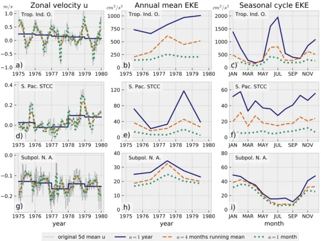
• 1-year a and b A more promising option to investigate interannual to decadal variations of the mesoscale is to choosea=b= 1 year. The changes of the mean currents at these time scales are not included in EKE and (2.10) holds. However, possible variations of the large scale circulation at seasonal time scales are still included in (u⁰, v⁰). The error made witha =b = 1 year depends on the region of interest. In regions with a strong seasonal cycle of the circulation such as the tropical Indian Ocean this error can be large and affect the interannual variability of EKE (Fig. 2.1a and b).

In other regions such as the subtropical South Pacific (Fig 2.1d and e) or the subpolar North Atlantic (Fig. 2.1g and h), the error is comparably small. Specifically, the mean EKE is affected by the inclusion of the seasonal cycle of the mean currents but the interannual and decadal variations of EKE remain of similar amplitude, relative to the respective mean. A detailed quantification of the error is not possible as all other methods described below impose errors as well, so that the discussion of the error

(22)

Figure 2.1: Different ways to calculate EKE as described in the text for three different regions:

(a)-(c) The tropical Indian Ocean (50^◦E,1^◦N) with a strong seasonal cycle of the mean current, (d)-(f) the subtropical South Pacific STCC (160^◦W,27^◦S) with relatively low EKE, and (g)-(i) the subpolar North Atlantic WGC (44^◦W,59^◦N) with strong EKE. The left column (a), (d), and (g) displays the original 5-day mean zonal velocity u (thin gray line), annual mean u (solid dark blue line), a 4-month running mean u (dashed orange line), and monthly mean u (dotted green line) for the arbitrary period 1 Jan. 1975 to 31 Dec. 1979. The center column (b), (e), and (h) shows annual mean EKE for the same period as calculated based on annual mean u (solid dark blue line), a 4-month running mean u (dashed orange line), and monthly mean u (dotted green line). The right column (c), (f), and (i) depicts the monthly seasonal cycle of EKE for the period 1970-1999. Colors and styles of the lines are identical to the center column. The details of the different methods to calculate EKE are described in the text.

needs to remain qualitative. A major disadvantage of b = 1 year is the impossibility to study the seasonal cycle of EKE. To overcome this shortcoming,b can be chosen to be 1 month.

• 1-year a and 1-month b Choosing a= 1 year and b= 1 month yields an additional error in the amplitude and phase of the seasonal cycle of EKE due to the term RES in (2.10) which is small in most regions, as already shown by Kang and Cur-

(23)

2.3 The Calculation of Eddy Kinetic Energy

chitser (2017). However, it can potentially be large in other regions, so that careful inspection is necessary before investigating the seasonal cycle of EKE. In the subpolar North Atlantic (Fig. 2.1i), all three methods yield similar mean and amplitude of the seasonal cycle. In the South Pacific STCC (Fig. 2.1f), the case wherea= 1 year and b= 1 month exhibits a similar phase of the seasonal cycle as the running mean a and the relative (to the mean) amplitude is comparable. In the tropical Indian Ocean (Fig.

2.1c), the timing of the seasonal cycle is comparable between all three methods, however, the relative amplitude is drastically increased (compared to the running meana) and a= 1 year, b = 1 month appears to be inadequate for the tropical Indian Ocean, where the seasonal cycle of the mean currents is large.

•1-monthaand b One possible solution to study the seasonal cycle of EKE without the introduction of the residual term in (2.10) is to seta=b= 1 month. However, this does not fully take into account the definition of the mesoscale. Using the de- viations (u⁰, v⁰) from monthly mean values implies that the mesoscale features under investigation have time scales shorter than one month. This assumption is not valid in most regions of the world’s oceans and indeed,a=b= 1 month yields a significant reduction of EKE and its variability in the tropics and subtropics (Fig. 2.1b, c, d, and f).

• Running mean a To include the full range of mesoscale variability in (u⁰, v⁰) and simultaneously study the seasonal cycle of EKE at a high resolution (as opposed to e.g. seasonal averages) it is possible to define a running mean window and filter the original time series of (u, v) do derive(u, v). However, this method still involves a residual term (Kang and Curchitser 2017) in (2.10) and additionally is computationally expensive compared to the other methods. Nevertheless, the error made by a running mean a appears to be the smallest of the errors associated with the methods discussed here and can serve as a reference for the other methods in Fig. 2.1.

The main features of Eddy Kinetic Energy investigated in this thesis are its interannual to decadal variations. With a focus on these long time scales, most results are derived utilizing annual or longer mean values of the quantities under consideration.

Furthermore, it is desirable to calculate EKE in the same manner everywhere, and for investigations of all time scales. In the subpolar North Atlantic, the region of focus of section 5, the amplitude and phasing of the temporal variations of EKE are almost

(24)

independent of the method chosen. In the subtropical South Pacific (focus of section 4), the different methods exert a larger influence on the EKE. Settinga=b = 1 month almost diminishes the seasonal and longer scale variations of EKE, in fact even the mean EKE is greatly reduced. Clearly, the choice of a= 1 month attributes parts of the mesoscale to (u, v) and is thus disregarded. When choosing a= 1 year and b= 1 year for the investigation of interannual to decadal variability andb = 1 month for the investigation of the seasonal cycle, the differences to the case where a is a running mean are mostly confined to the average EKE. The effects on the relative amplitudes and the phase of variations and the seasonal cycle are only minor. Addi- tionally, the running mean method has the disadvantage of the computational expense, which is considered more important than its better accuracy at this point. Thus, to ensure EKE is efficiently calculated in the same way for all regions, a= 1 year in the remaining sections of this thesis. When focusing on interannual to decadal variability b= 1 year, and b= 1 month for the investigation of the seasonal cycle.

It should be noted that the insights gained in this thesis do not depend on the choice of a and b. All methods but a=b= 1 month yield similar variations relative to the mean EKE at seasonal, interannual, and decadal time scales in the subtropical South Pacific and the subpolar North Atlantic. In the regional context of this study, the method used to derive EKE is thus not critical to the investigation of the time scales considered. Only when a comparison of the energy of the mesoscale and the mean circulation, i.e. EKE and MKE, is required, does the choice ofa and b become essential.

In the subtropical South Pacific for example, EKE is 7 times as large as MKE when a=b= 30 years (not shown). In the case a=b= 1 year this factor reduces to 6 and for a=b = 1 month EKE and MKE are almost identical. Depending on the method chosen, it could be claimed that EKE is an order of magnitude larger than MKE or that they are of similar magnitude. Therefore, it is essential to carefully choose the averaging periods a and b for the calculation of EKE depending on the investigated region and the processes to study.

(25)

3 On the Influence of Lateral Diffusion of

Momentum on Eddy Kinetic Energy in an Ocean General Circulation Model

3.1 Background

The technological advances of the recent decades make it possible today to integrate Ocean General Circulation Models in global configurations at high resolutions of 1/10^◦ and higher for simulation periods of up to a few decades (e.g. Smith et al. 2000; Mal- trud and McClean 2005; Sasaki et al. 2008; Deshayes et al. 2013; Rieck et al. 2015;

Sérazin et al. 2015). One of the key advantages of these high-resolution OGCMs is their ability to simulate the oceanic mesoscale and its effects on the ocean’s climate at a wide range of latitudes (cf. Hallberg 2013). However, even by today’s standards, OGCMs with resolutions finer than 1/10^◦ are computationally expensive and under certain circumstances it is favorable to use a model with a coarser resolution, depending on the processes to investigate and the latitudinal range involved. The major benefits of coarser-resolution OGCMs is the possibility to extend the simulation length and conduct sensitivity studies to investigate different parameter spaces or the influence of certain aspects of the atmospheric forcing. To exploit these benefits, section 3 and 4 of this thesis are based on an eddy-permitting 1/4^◦ OGCM.

A 1/4^◦ OGCM should be able to resolve the first baroclinic Rossby radius of deformation and thus at least parts of the mesoscale variability from the equator to roughly 20−25^◦ North and South (Chelton 1998). Earlier studies utilizing 1/4^◦ configurations exhibit mesoscale eddies and variability well into the midlatitudes (e.g. Penduff et al.

2010; Sérazin et al. 2015), although less of the range of mesoscale features is resolved the further poleward the area of investigation is located. It thus seems promising to use a 1/4^◦ OGCM to investigate mesoscale variability in the subtropics and at the same time carry out sensitivity studies with variations to the atmospheric forcing and some tests with changing model parameters. One of the most challenging parameters to define, especially within an eddy-permitting model, is the lateral diffusion of momentum that will be discussed here.

(26)

Physically, momentum is dissipated by friction on the molecular scale. As ocean models do not resolve such small scales, a viscosity parametrization is implemented to account for the transfer of energy toward smaller scales and its dissipation. A second role of the viscosity is to ensure numerical stability of the model. Depending on the horizontal resolution, the resolved dynamical processes flux a certain amount of energy to smaller scales which then is essentially trapped at the grid-scale. The viscosity parametrization acts to dissipate this energy at the grid-scale and suppresses the growth of unstable waves that could potentially lead to a blow-up of the model.

Most advection schemes implemented in model formulations yield some additional numerical dissipation of energy, but this aspect is not discussed here in detail.

In very high-resolution models that resolve ocean dynamics down to the scale at which the direction of the energy flux changes from upscale to downscale (e.g. Scott and Wang 2005), the role of the parametrization of lateral viscosity of momentum is relatively straight-forward to assign. The energy flux from smaller scales to larger scales is explicitly simulated by the model and the viscosity parametrization only needs to account for the flux toward smaller scales that are not resolved by the model and the dissipation at the molecular scale.

In coarse-resolution models (0.5^◦ and lower) the mesoscale is not resolved. Both the effect of mesoscale eddies on the large-scale oceanic properties and the flux of energy toward small scales can be parametrized though. Gent and Mcwilliams (1990) show one example for the parametrization of the effect of mesoscale eddies. Their parametrization essentially aims at mimicking baroclinic instability with the help of an additional eddy-induced advection velocity, reducing the lateral gradients of tracers and the available potential energy. The flux of energy to the small scales is, as in high-resolution models, approximated by the viscosity. In coarse-resolution models the parametrized viscosity removes energy from scales that are much larger than physically realistic. However, this deficiency can be partly counteracted because the oceanic mesoscale and its effect on the larger scales are parametrized, and thus controllable, as well.

The most problematic case with respect to the choice of lateral viscosity is the case of intermediate resolution between 1/3^◦ and 1/10^◦, 1/4^◦ in this study. At 1/4^◦, the mesoscale is partly resolved, at least in the tropics and subtropics. Thus, the grid-scale of the model configuration lies within the mesoscale range and energy from this grid-

(27)

3.1 Background

scale could be fluxed to larger scales. However, numerical dissipation and viscosity in its most common forms only dissipate energy, i.e. parametrize the flux of energy to smaller scales, and thus do not account for the mesoscale’s effect on the large-scale.

Due to this contradiction, the choice of lateral viscosity in eddy-permitting ocean models is a delicate one. On the one hand, the viscosity needs to be large enough to assure that energy does not accumulate at the grid-scale. On the other hand, the viscosity should be chosen as small as possible to allow a free evolution of the dynamical features resolved by the model.

Several constraints, based on theoretical considerations, limit the choice of an adequate magnitude of the lateral viscosity of momentum. An upper bound is given by a criterion for numerical stability, the viscous Courant-Friedrichs-Levy criterion (Jochum et al. 2008). This upper bound should be adhered to in order to avoid the possibility of diffusion of momentum across more than one grid cell in one time step. Further- more, there are two constraints on the lower bound of an adequate lateral viscosity (Bryan et al. 1975; Large et al. 2001). First, the Grid-Reynolds number should not exceed some thresholdαin order to suppress grid-scale noise. In the case of advection schemes based on centered differences,α = 2for second-order diffusive operators and α = 16 for fourth-order diffusive operators (Griffies and Hallberg 2000). Second, the grid needs to resolve the Munk boundary layer (Munk 1950). This boundary layer is determined by the ratio of the viscosity and the planetary vorticity gradient. Essen- tially, the Munk boundary layer becomes thinner for decreasing vorticity and the grid spacing needs to be chosen adequately to resolve it. Or, when the grid-spacing is fixed, the viscosity should not decrease below a certain threshold.

The upper and lower theoretical bounds for the viscosity parameter still leave a range of possible choices that is additionally influenced by the numerical diffusion of the advection scheme. The numerical diffusion is often unknown and hard to assess (e.g. Ilıcak 2016) so that a careful testing of different viscosity parameters is necessary to find an adequate value and achieve the best results. A rather large viscosity near the upper limit ensures a minimum of numerical noise and thus reduces spurious, undesirable diapycnal mixing of tracers (Megann 2018). At the same time, the stronger diffusion of momentum weakens gradients across fronts and could potentially decrease the generation of instabilities and mesoscale variability. Especially in an eddy-permitting simulation, e.g. the 1/4^◦ simulation used in this study, the viscosity should be kept as low as possible in order to benefit from the partly resolved mesoscale and its effects on

(28)

the large-scale circulation. Indeed, reducing the viscosity has been shown to increase Eddy Kinetic Energy (Böning et al. 1991) and improve the representation of many large-scale currents (Jochum et al. 2008) in eddy-permitting models. Jochum et al.

(2008) even argue that violating some of the theoretical constraints mentioned above can be beneficial to eddy-permitting simulations. Specifically, the advantages of a more vigorous eddy field and its effect on the mean currents can potentially outweigh the disadvantages of an increased level of grid-scale noise.

Based on these considerations, the effect of a reduced lateral viscosity on EKE in the eddy-permitting ocean model configuration used in section 4 of this thesis is investigated in this section. The aim is to optimize the simulation’s ability to represent mesoscale variability without developing an excessive amount of grid-scale noise. The regional focus is on the subtropical South Pacific, the study region of section 4.

3.2 Model Configuration

The specific configuration of the model (described in section 2) used in this section is global and eddy-permitting at a horizontal resolution of 1/4^◦ (ORCA025). It has an orthogonal, curvilinear, tripolar Arakawa-C type grid, shared with the numerous varieties of the ORCA025 configuration developed within the DRAKKAR framework (DRAKKAR Group 2007, 2014). The version of ORCA025 used in this study has 46 vertical levels with increasing thickness toward the ocean bottom. The surface grid cell is 6m and cells at depth are up to ∼250 m thick, with 24 (9) of the 46 cells being located in the upper 1000 m (100 m). A partial-cell formulation is applied for the bottom cells (cf. Barnier et al. 2006). The data products and bulk formulations of the Coordinated Ocean-Ice Reference Experiments version 2 (CORE.v2) are used to atmospherically force the simulations (see section 2 for a detailed description of CORE.v2). All model simulations apply a very weak sea surface salinity restoring (SSSR) to climatology (PHC2.1, updated from Steele et al. 2001) of33.33mm day⁻¹, which corresponds to a relaxation time scale of 1500 days over a 50 m surface layer.

The presented configuration of ORCA025 uses a bilaplacian horizontal diffusion for momentum. The fourth order diffusive operator from the momentum equations (see

(29)

3.2 Model Configuration

section 2) is given by (see Madec 2008) D^lU =∇_h

∇_h·

−A^lm∇_h(χ)

+∇_h×

k· ∇ ×

−A^lm∇_h×(ζk)

(3.1)

where ∇_h = _e¹

1

∂

∂ii+_e¹

2

∂

∂jj, A^lm is the viscosity coefficient, i, j, and k are the unit vectors (k locally upward), and χ and ζ are the divergence of the horizontal velocity field and the relative vorticity, respectively, given by

χ= 1 e1e2

∂(e₂u)

∂i +∂(e₁v)

∂j

(3.2)

ζ = 1 e₁e₂

∂(e2v)

∂i − ∂(e1u)

∂j

(3.3) Here, e₁ and e₂ are the horizontal scale factors, i.e. the lengths of the grid cell in i- and j-direction, respectively. The horizontal velocities in i- and j-direction are denoted byu and v, respectively. The viscosity coefficient A^lm depends on the size of the grid cell considered.

A^lm = max(e₁, e₂)³

e³_max A^lm₀ (3.4)

wheree_max is the global maximum of all horizontal scale factors e₁ and e₂ in the grid configuration and A^lm₀ is the background viscosity coefficient. If all grid cells were the same size, A^lm =A^lm₀ everywhere. In ORCA025 however, grid cells are largest at the equator and decrease in size toward the poles, so that A^lm also decreases from A^lm₀ at the equator to smallest values near the poles of the tripolar grid. The background viscosity coefficient A^lm₀ (hereafter simply called viscosity) is varied in the different simulations conducted. A viscosity of A^lm₀ =1.5×10¹¹ m⁴s⁻² has been widely used in previous simulations with ORCA025 and acts a standard value for the control experiments V15 (spin-up experiment) and V15H (hindcast simulation) here. Three additional experiments are analyzed. A combination of a spin-up (V06) and a hindcast simulation (V06H) with a reduced viscosity of A^lm₀ =0.6×10¹¹ m⁴s⁻² and a short spin-up experiment with very low viscosity A^lm₀ =0.2×10¹¹ m⁴s⁻² (V02). While all three values for the viscosity, 1.5, 0.6, and 0.2×10¹¹ m⁴s⁻², lie well below the upper bound for adequate values given by the viscous Courant-Friedrichs-Levy criterion, only 1.5×10¹¹ m⁴s⁻² fulfills the Grid Reynolds number criterion, and none of them strictly adheres to the Munk boundary layer criterion. However, as mentioned above, these viscosity parameterizations do not take into account the additional numerical diffusion by the advection scheme, so that the actual diffusion acting upon the momentum in

(30)

the simulation is higher and a stable model integration could be possible with these low values of the viscosity parameter.

In V02, the horizontal diffusion coefficient for tracers is additionally adapted to the lower viscosity for momentum. The ORCA025 simulations analyzed in this study use a laplacian diffusive operator of the form

D^lT =∇ · A^lt < ∇T

with <=







1 0 −r₁ 0 1 −r₂

−r₁ −r₂ r₁²+r₂²





 (3.5)

whereA^ltis the diffusion coefficient that (as for momentum in Eq. 3.4) depends on the local grid cell size,T is the tracer field and r₁ and r₂ are the slopes between isoneutral surfaces and the model’s vertical level in the i- and j-direction, respectively. Analo- gously to the diffusion of momentum, there is a background value A^lt₀ for the tracer diffusion coefficient A^lt. The standard value of A^lt₀ in V15, V15H, V06, and V06H is 300 m²s⁻¹. In V02 however, the viscosity for momentum is reduced drastically, so thatA^lt₀ is changed to 100 m²s⁻¹ to avoid that the diffusion for momentum and tracers differs strongly.

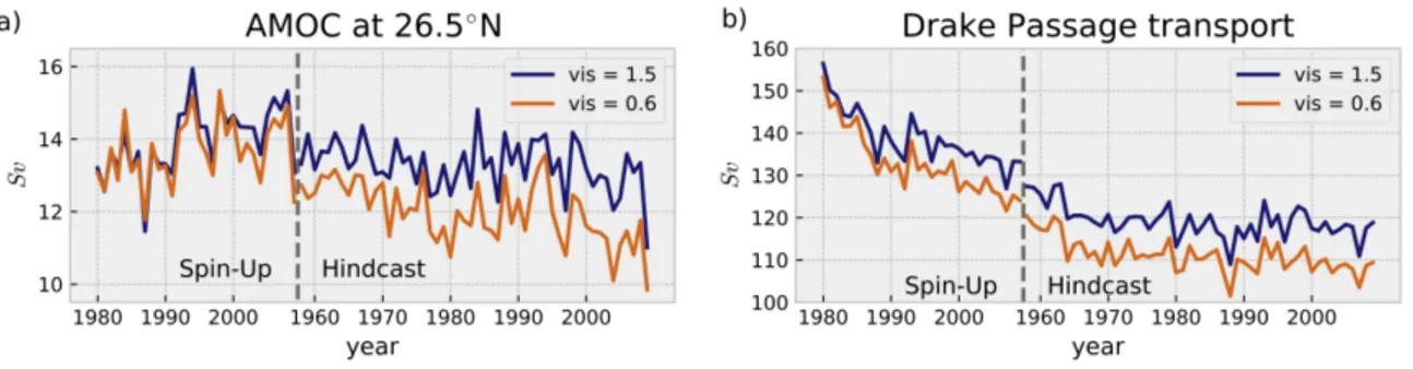
The three different spin-up simulations V15, V06 and V02 are initialized with temperature and salinity from climatology (PHC2.1, updated from Steele et al. 2001) and a sea ice field from December 31st, 1992 from a previous ORCA025 simulation. First, the three simulations, only differing in their choices of diffusion coefficients, are integrated for 5 years, forced by the CORE.v2 atmospheric forcing from 1 January 1980 to 31 December 1984. The spin-up integrations for V15 and V06 are then continued for another 25 years until 31 December 2009. The state of the ocean at the end of this spin-up period is then used as the initial condition for the two hindcast simulations V15H and V06H. The hindcast simulations are integrated for 52 years with the forcing from 1 January 1958 to 31 December 2009.

(31)

3.3 Results

Figure 3.1:(a) Zonal mean (153−175^◦W) EKE (cm²s⁻²) at 94 m depth, averaged over 3 years from 1982−1984, for three different lateral viscosities. 1.5×10¹¹m⁴s⁻² (V15; solid blue line), 0.6×10¹¹ m⁴s⁻² (V06; dashed orange line), and 0.2×10¹¹ m⁴s⁻² (V02; dash-dotted green line).

(b) as (a) but for small-scale squared zonal velocity U²(cm²s⁻²). Zonal velocities are filtered in the zonal and meridional directions with a boxcar window with the size of 2 grid cells and then subtracted from the original field to retain small-scale velocities.

3.3 Results

The aim of this section is to characterize and quantify the changes to EKE in the STCC and the large scale hydrographic properties and circulation resulting from different values of the viscosity parametrization. The underlying question is whether it is possible to optimize the models simulation of the mesoscale without increasing the grid-scale noise above an acceptable level.

The EKE in the subtropical South Pacific generally exhibits an increase when decreasing the model’s viscosity (Fig. 3.1a). Zonally averaged from 153−175^◦W, EKE at 94 m depth in the V06 case is up to 15 cm²s⁻² (50%) higher in the latitude range of the STCC (∼23−30^◦S) when compared to V15. Outside the STCC the changes are only minor. In V02, EKE increases by 30 cm²s⁻² (100%) in the STCC, with respect to V15. In all three simulations, the meriodional structure of the STCC system remains unchanged with a sharp increase of EKE between 35 and 30^◦S, two peaks of EKE at roughly 28 and 25^◦S accompanied by a local minimum between these latitudes, and a decrease of EKE between 25 and 20^◦S.

(32)

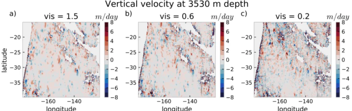
Figure 3.2: Snapshots (5-day mean) of vertical velocity (m day⁻¹) at 3530 m depth in the South Pacific for (a) V15 (viscosity of 1.5×10¹¹ m⁴s⁻²), (b) V06 (viscosity of 0.6×10¹¹m⁴s⁻²), and (c) V02 (viscosity of 0.2×10¹¹ m⁴s⁻²).

While an increase of EKE to levels as simulated by a 1/10^◦-simulation (see section 4.3.4) seems desirable, care has to be taken when interpreting these results. Indeed, most of the additional EKE observed in V02 stems from velocity anomalies near the grid-scale. To quantify these small-scale velocities, the zonal velocity U is filtered in the zonal and meridional directions with a boxcar window with the length of 2 grid cells (the filtered value in each cell is the mean of the unfiltered value of this cell and the cell to the west and south, respectively). These filtered fields are then subtracted from the original fields, so that only anomalies near the grid-scale are retained. These small-scale anomalies are then squared and zonally averaged (Fig. 3.1b).

The small-scale velocities in V06 are only locally larger than in V15. The maximum increases observed within the STCC (∼23-31^◦S) do not exceed 2−4cm²s⁻². In V02 however, small-scale velocities are significantly increased between 15− 36^◦S. In the STCC small-scale U² is up to 14 cm²s⁻² larger in V02 as compared to V15. This drastic increase on the order of 300−400% questions the usability of V02 for long, realistic hindcast simulations.

To further investigate the effect of low viscosity on grid-scale noise, the vertical velocities are studied. Vertical velocities are very sensitive to grid-scale noise in the model configuration because they are calculated diagnostically from the divergence of the horizontal velocities, simplified −dw/dz =du/dx+dv/dy. The influence of horizontal velocities with alternating sign from cell to cell that are characteristic of grid scale noise is thus well observable in the vertical velocities, especially near topography, where vertical velocities are generally larger.

(33)

3.3 Results

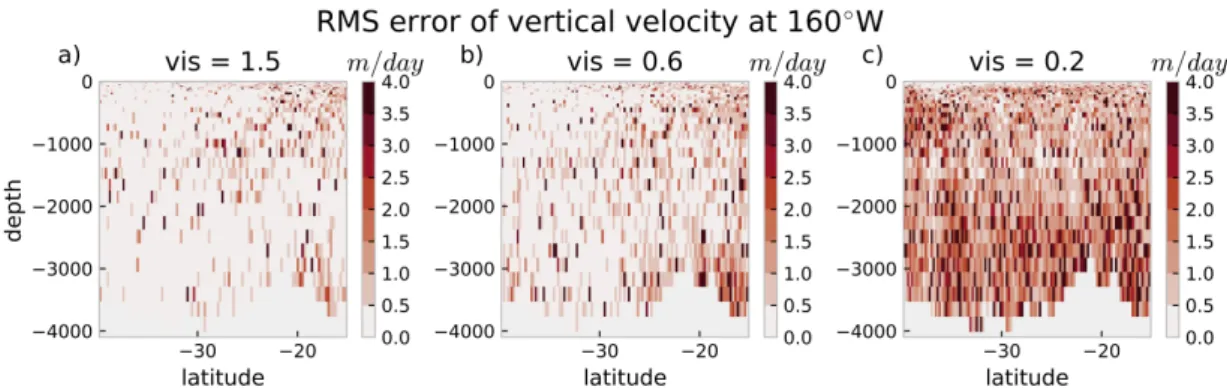
Figure 3.3:Vertical sections of the RMS error of vertical velocity wRM S (m day⁻¹) at 160^◦W, averaged over 3 years (1982−1984) for (a) V15 (viscosity of 1.5×10¹¹m⁴s⁻²), (b) V06 (viscosity of 0.6×10¹¹ m⁴s⁻²), and (c) V02 (viscosity of 0.2×10¹¹m⁴s⁻²). wRM S is calculated as described in the text.

The vertical velocities in the interior basins at 3530 m depth, away from topography are generally below 2 m day⁻¹ (Fig. 3.2). In V15 higher velocities are found e.g. near the ridges in the northwestern part of the investigated region. At some locations (for example between 140−150^◦W, near 25^◦S) the typical pattern of grid-scale noise can be observed even with the standard viscosity parametrization. In V06, the vertical velocities in the interior are not changed significantly, whereas grid-scale noise can be seen close to all the topographic features in the region at a slightly increased level compared to V15. For the low viscosity case, the majority of vertical velocities can be attributed to noise. Close to topography, the velocities often exceed 10 m day⁻¹ and the typical pattern of velocities of alternating sign in neighboring grid cells can be observed hundreds of kilometers away.

To better quantify the amount of grid-scale noise, the vertical velocities are vertically smoothed with a 5-point Hanning window (w_smooth) and a root-mean-square (RMS) error is calculated.

w_{RM S} =

r(w−w_smooth)² w²

(3.6) Here,h·idenotes a temporal mean. This approximation of grid-scale noise is displayed in Figure 3.3. For V15, there are low levels of noise in most of the region, with only slightly increased levels north of 25^◦S in the upper ocean and near the ridge north of 20^◦S in the deep ocean. Average values of the RMS error are 0.58 m day⁻¹ for the upper 1000 m and 0.37 m day⁻¹ for the depths below 1000 m. Decreasing the