SIMIP Community∗
2
(Detailed listing according to AGU guidelines for community papers is in the
3
appendix. Repeated here for reference: Dirk Notz, Jakob D¨orr, David A
4
Bailey, Ed Blockley, Mitchell Bushuk, Jens Boldingh Debernard, Evelien
5
Dekker, Patricia DeRepentigny, David Docquier, Neven S. Fuˇckar, John C.
6
Fyfe, Alexandra Jahn, Marika Holland, Elizabeth Hunke, Doroteaciro Iovino,
7
Narges Khosravi, Fran¸cois Massonnet, Gurvan Madec, Siobhan O’Farrell,
8
Alek Petty, Arun Rana, Lettie Roach, Erica Rosenblum, Clement Rousset,
9
Tido Semmler, Julienne Stroeve, Bruno Tremblay, Takahiro Toyoda, Hiroyuki
10
Tsujino, Martin Vancoppenolle)
11
Key Points:
12
• CMIP6 model simulations of Arctic sea-ice area capture the observational record
13
in the multi-model ensemble spread
14
• The sensitivity of Arctic sea ice to changes in the forcing is better captured by CMIP6
15
models than by CMIP5 and CMIP3 models
16
• The majority of available CMIP6 simulations lose most September sea ice for the
17
first time before 2050 in all scenarios
18
∗See appendix for detailed listing
Corresponding author: Dirk Notz,dirk.notz@uni-hamburg.de
7KLVDUWLFOHKDVEHHQDFFHSWHGIRUSXEOLFDWLRQDQGXQGHUJRQHIXOOSHHUUHYLHZEXWKDVQRW EHHQWKURXJKWKHFRS\HGLWLQJW\SHVHWWLQJSDJLQDWLRQDQGSURRIUHDGLQJSURFHVVZKLFKPD\
OHDGWRGLIIHUHQFHVEHWZHHQWKLVYHUVLRQDQGWKH9HUVLRQRI5HFRUG3OHDVHFLWHWKLVDUWLFOHDV
GRL*/
Abstract
19
We examine CMIP6 simulations of Arctic sea-ice area and volume. We find that CMIP6
20
models produce a wide spread of mean Arctic sea-ice area, capturing the observational
21
estimate within the multi-model ensemble spread. The CMIP6 multi-model ensemble
22
mean provides a more realistic estimate of the sensitivity of September Arctic sea-ice area
23
to a given amount of anthropogenic CO2emissions and to a given amount of global warm-
24
ing, compared with earlier CMIP experiments. Still, most CMIP6 models fail to simu-
25
late at the same time a plausible evolution of sea-ice area and of global mean surface tem-
26
perature. In the vast majority of the available CMIP6 simulations, the Arctic Ocean be-
27
comes practically sea-ice free (sea-ice area<1 million km2) in September for the first
28
time before the year 2050 in each of the four emission scenarios SSP1-1.9, SSP1-2.6, SSP2-
29
4.5 and SSP5-8.5 examined here.
30
Plain Language Summary
31
We examine simulations of Arctic sea ice from the latest generation of global cli-
32
mate models. We find that the observed evolution of Arctic sea-ice area lies within the
33
spread of model simulations. In particular, the latest generation of models performs bet-
34
ter than models from previous generations at simulating the sea-ice loss for a given amount
35
of CO2 emissions and for a given amount of global warming. In most simulations, the
36
Arctic Ocean becomes practically sea-ice free (sea-ice area<1 million km2) in Septem-
37
ber for the first time before the year 2050.
38
1 Introduction
39
In recent decades, Arctic sea-ice area has decreased rapidly, and the signal of a forced
40
sea-ice retreat has clearly emerged from the background noise of year-to-year variabil-
41
ity. Because of this, the ability of climate models to plausibly simulate the observed changes
42
in Arctic sea-ice coverage has become a central measure of model performance in Arctic-
43
focused climate model intercomparisons (e.g., Koenigk et al., 2014; Massonnet et al., 2012;
44
Melia et al., 2015; Olonscheck & Notz, 2017; Shu et al., 2015; Stroeve et al., 2007, 2012,
45
2014). In this contribution, we extend these earlier studies that examined model perfor-
46
mance in the third and fifth phases of the Coupled Model Intercomparison Project (CMIP3
47
and CMIP5) by examining model simulations from the sixth phase of the Coupled Model
48
Intercomparison Project (CMIP6, Eyring et al., 2015). For CMIP6, the Sea-Ice Model
49
Intercomparison Project (SIMIP, Notz et al., 2016) designed a specific set of diagnos-
50
tics that allow for detailed analyses of sea-ice related processes and thus a process-based
51
evaluation of sea-ice simulations of the participating models. To lay the foundation for
52
such analyses, we here provide an initial overview of CMIP6 model performance by ex-
53
amining some large-scale, pan-Arctic metrics of model performance and future sea-ice
54
evolution, including a comparison to CMIP5 and CMIP3 simulations. A similar anal-
55
ysis for Antarctic sea ice is given by (Roach et al., under review).
56
2 Analysis Method
57
In this contribution, we examine two large-scale integrated quantities that describe
58
the time evolution of Arctic sea ice. These are the Northern Hemisphere total sea-ice area
59
(SIA) and total sea-ice volume (SIV), which can be calculated readily from SIMIP vari-
60
ables as follows.
61
To obtain sea-ice area for CMIP6 model simulations, we use the SIMIP variable
62
of Northern Hemisphere sea-ice areasiareanwhen provided. If siareanis not provided,
63
we calculate the sea-ice area by multiplying sea-ice concentration on the ocean grid (siconc,
64
preferred) or on the atmospheric grid (siconca) with individual grid-cell area and then
65
sum over the Northern Hemisphere. Note that we use sea-ice area as our primary vari-
66
able to describe sea-ice coverage instead of sea-ice extent, which is usually calculated as
67
the total area of all grid cells with at least 15% sea-ice concentration. Our choice to fo-
68
cus on sea-ice area derives primarily from the fact that sea-ice extent is a strongly grid-
69
dependent, non-linear quantity, making it difficult to meaningfully compare between model
70
output and satellite observations (compare Notz, 2014). In addition, the observational
71
spread across different satellite products is smaller for trends in sea-ice area than it is
72
for trends in sea-ice extent (Comiso et al., 2017).
73
To calculate sea-ice volume for CMIP6 models, we (1) directly use the SIMIP vari-
74
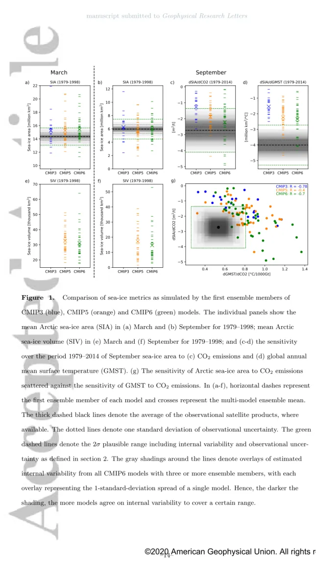
able of Northern Hemisphere sea-ice volumesivolnwhen provided, or (2) multiply the
75
sea-ice volume per grid-cell areasivolby individual grid-cell area and sum over the North-
76
ern Hemisphere, or (3) multiply sea-ice-concentrationsiconc, sea-ice thicknesssithick
77
and individual grid-cell area and then sum over the Northern Hemisphere. For CMIP5,
78
only the sea-ice volume per grid-cell area (also called “equivalent sea-ice thickness”,sit)
79
ice volume data for CMIP3 models, so volume comparisons in the following are limited
81
to CMIP5 and CMIP6 model simulations.
82
To meaningfully estimate model performance relative to the real evolution of the
83
sea-ice cover in the Arctic, we must take internal variability into account (see, for ex-
84
ample, England et al., 2019; Kay et al., 2011; Notz, 2015; Olonscheck & Notz, 2017; Swart
85
et al., 2015). Internal variability describes the spread in plausible climate trajectories
86
in response to a given forcing scenario, owing to the chaotic nature of our climate sys-
87
tem. The observational record is just one such plausible trajectory, and no single model
88
simulation can ever be expected to perfectly agree with it because of its chaotic nature.
89
Therefore, most CMIP6 models have been run several times with slightly different ini-
90
tial conditions to estimate the range of trajectories that are compatible with a given model’s
91
physics. In the following, we take two different approaches to examine whether a given
92
model provides a plausible simulation of the observational record in light of internal vari-
93
ability.
94
First, for CMIP6 models, we estimate a best-guess CMIP6-average internal vari-
95
abilityσcmip6 by averaging across the individual ensemble spread of those models that
96
provide three or more ensemble members (see Table S3 for details). In calculating the
97
standard deviation, we correct for small sample sizenby using Bessel’s correction and
98
then dividing the resulting standard deviation by the scale mean of the chi distribution
99
withn−1 degrees of freedom. We then define all simulations that lie within the range
100
of 2σ=±2q
σ2cmip6+σ2obsaround the observational estimate as plausible simulations
101
(compare Olonscheck & Notz, 2017). Here,σ2obsrefers to the observational uncertainty
102
explained below. This approach allows us to also examine the plausibility of those mod-
103
els that only provide a single ensemble member. In addition to considering internal vari-
104
ability explicitly, we reduce its impact by examining model performance relative to a time
105
average over several years. We take the first twenty years of the satellite record (1979–
106
1998) for comparing mean values, as those twenty years provide a compromise between
107
using as many years as possible and using a period with no strong trend in Arctic sea-
108
ice area and volume. However, even on multi-decadal time scales internal variability af-
109
fects the Arctic sea-ice cover, so averaging over 20 years is not long enough an averag-
110
ing period to remove the impact of internal variability entirely. To compare trends, we
111
examine the overlap period 1979–2014 of the satellite record, which begins in 1979, and
112
the historical period of CMIP6, which ends in 2014.
113
Second, in order to select a subset of models for estimating a best guess of the fu-
114
ture evolution of the Arctic sea-ice cover, we take the more strict approach to define a
115
model as plausible if its ensemble spread includes the observational record, considering
116
observational uncertainty. These models are referred to as “selected models” hereafter.
117
To obtain an observational estimate of sea-ice area, we use observational records
118
of sea-ice concentration from the OSI SAF (Lavergne et al., 2019), NASA-Team (Cavalieri
119
et al., 1997) and Bootstrap (Comiso et al., 1997) algorithms. Sea-ice area is then cal-
120
culated by multiplying the sea-ice concentration with individual grid-cell area and sum-
121
ming over the Northern Hemisphere. For the NASA-Team and Bootstrap algorithms,
122
we filled the observational pole hole with the average sea-ice concentration around its
123
edge (Olason & Notz, 2014). For OSI SAF, we used the filled pole hole of the product
124
itself. We take the spread of the three algorithms obtained this way as the observational
125
uncertaintyσobs.
126
For sea-ice volume, we do not compare models with an observational estimate due
127
to substantial uncertainties for reanalysed and observed estimates of Arctic sea-ice thick-
128
ness and thus volume (e.g. Bunzel et al., 2018; Chevallier et al., 2017; Zygmuntowska
129
et al., 2014).
130
For global-mean surface temperature (GMST), we use the average of NOAAGlob-
131
alTemp v5.0.0 (Vose et al., 2012), GISTemp v4 (GISTEMP Team, 2019; Lenssen et al.,
132
2019), HadCRUT4.6.0.0 (Morice et al., 2012) and Berkeley (Rohde et al., 2013) time-
133
series as an estimate for the mean evolution, and the spread across these four records
134
as an estimate for observational uncertainty. We calculate anomalies relative to the pe-
135
riod 1850–1900, except for the shorter record of NOAAGlobalTemp where we calculate
136
anomalies relative to 1880–1900. Because the 20-year running-mean temperature fluc-
137
tuations during these periods are less than 0.1◦C, our results are largely insensitive to
138
this choice of baseline period (Figure S2). We take the spread of the four products as
139
the observational uncertaintyσobs.
140
Historical anthropogenic CO2 emissions are taken from the historical budget of (Global
141
Carbon Project, 2019). Future anthropogenic CO2 emissions for CMIP6 simulations are
142
taken from the respective SSP scenarios described by (Riahi et al., 2017).
143
3 CMIP6 Model Performance
144
3.1 Mean Quantities
145
We start with an analysis of the mean sea-ice fields simulated by individual CMIP3,
146
CMIP5 and CMIP6 models (Figure 1a, b, e, f) over the period 1979–1998. To allow for
147
a fair comparison across the three CMIP phases, in this section we analyze only the first
148
ensemble member of each model. Given the large number of participating models, this
149
results in a fair comparison: for models with several ensemble members, the first ensem-
150
ble member is as likely to be above a model’s ensemble mean as below.
151
For sea-ice area, we find a large spread across CMIP6 simulations both in March
152
and in September (Figure 1a, b), which usually are the months of maximum and min-
153
imum sea-ice coverage in the Arctic, respectively. In March, the 1979–1998 mean sea-
154
ice area simulated by CMIP6 models ranges from around 12 million km2to more than
155
20 million km2 and thus includes the observational estimate of 14.4 million km2 (Fig-
156
ure 1a, Table S3). Out of the 40 CMIP6 models, 21 are within the 2σ=±1.29 million
157
km2 plausibility range around the observational estimate given by the CMIP6-average
158
internal variability and observational uncertainty as introduced in section 2 (Figure 1a,
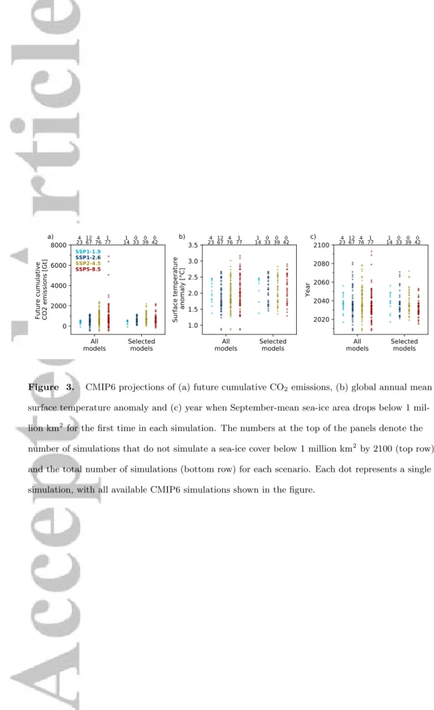
159
Table S3). CMIP3 and CMIP5 simulations also show a large spread in mean March sea-
160
ice area, and include the observational estimate within their multi-model ensemble spread
161
(Figure 1a, Tables S1 and S2). However, in CMIP3 and CMIP5, the multi-model ensem-
162
ble spread is more evenly distributed around the observational estimate than in CMIP6,
163
where most models lie above it.
164
For the mean September sea-ice area over the period 1979–1998, the CMIP6 en-
165
semble also shows a large spread of individual simulations, ranging from around 3 mil-
166
lion km2 to around 10 million km2 (Figure 1b, Table S3). The observed value of around
167
6 million km2 lies well within the range, and 25 out of 40 CMIP6 models are within the
168
plausible range of 2σ=±1.49 million km2 around this value (Table S3). The CMIP6
169
multi-model ensemble mean is very close to the observational estimate and well within
170
the plausible range. The same holds for CMIP3 and CMIP5, with their individual mod-
171
els also spanning a wide range around the observational estimate (Figure 1b, Tables S1
172
and S2).
173
For sea-ice volume, we lack data for CMIP3 models and thus can only compare CMIP6
174
results to CMIP5 results (see tables S2 and S3 for a detailed overview). For both phases
175
of CMIP, the models produce a similar spread of simulated Arctic sea-ice volume from
176
less than 20,000 km3 to more than 40,000 km3 in March (Figure 1e), and from less than
177
5,000 km3 to more than 30,000 km3 in September (Figure 1f). Given a simulated aver-
178
age spread from internal variability of around 2,000 km3, the large spread in sea ice vol-
179
ume from CMIP6 models can not be explained by internal variability alone. Instead, it
180
is caused by the models’ large spread in simulated sea-ice area and thickness.
181
Based on this analysis of mean Arctic sea-ice quantities, we find that there is lit-
182
tle difference in overall model performance between CMIP3, CMIP5 and CMIP6. The
183
multi-model spread of the mean quantities remains large, the observational record lies
184
within the multi-model ensemble spread, and many models simulate plausible values of
185
mean sea-ice area when considering the impact of internal variability and observational
186
uncertainty. The multi-model ensemble means of the past three phases of CMIP are rel-
187
atively similar to each other and largely consistent with the observational record.
188
3.2 Sensitivity
189
In addition to their plausible simulation of mean quantities, the models’ adequacy
190
for simulating reality hinges critically on their ability to realistically simulate the response
191
of a given climate metric to changes in external forcing. Internal variability causes a large
192
spread of plausible climate trajectories in response to a given change in the forcing and
193
must carefully be taken into account when interpreting a possible mismatch between a
194
simulation and a given observational sea-ice record (Jahn et al., 2016; Kay et al., 2011;
195
Notz, 2015; Olonscheck & Notz, 2017; Swart et al., 2015). We find this to remain valid
196
for CMIP6 simulations.
197
For our analysis of the simulated sensitivity of Arctic sea ice to changes in exter-
198
nal forcing, we calculate two distinct quantities: first, the change in sea-ice area for a given
199
change in cumulative anthropogenic CO2 emissions over the period 1979–2014 (Figure
200
1c); second, the change in sea-ice area for a given change in global mean surface tem-
201
perature (GMST) over the period 1979–2014 (Figure 1d). Both quantities can be cal-
202
culated from the previously demonstrated linear relationships of sea-ice area to cumu-
203
lative CO2 emissions (Herrington & Zickfeld, 2014; Notz & Stroeve, 2016; Zickfeld et al.,
204
2012) and to GMST (e.g., Gregory et al., 2002; Mahlstein & Knutti, 2012; Rosenblum
205
& Eisenman, 2016; Stroeve & Notz, 2015; Winton, 2011). Together, these two quanti-
206
ties allow us to estimate whether CMIP6 models simulate changes in sea ice with the cor-
207
rect sensitivity to changes in external forcing, and whether they potentially do so for the
208
right reason. This is because the relationship between sea-ice area and cumulative an-
209
thropogenic CO2 emissions is an almost linear proxy for the long-term time evolution
210
of Arctic sea-ice area, as cumulative emissions map monotonously to time. In contrast,
211
the sensitivity of sea-ice area to GMST changes is a proxy for the sensitivity of the sea-
212
ice cover to one particular response of the climate system to changes in external forc-
213
ing.
214
Our analysis reveals that over the historical period 1979–2014, 28 out of 40 CMIP6
215
models simulate a sensitivity of the Arctic sea-ice area to cumulative anthropogenic CO2
216
emissions that is within the plausible range of 2.73±1.37 m2of sea-ice loss per ton of CO2
217
emissions (Figure 1c, Table S3). In addition to the larger spread of the CMIP6 multi-
218
model ensemble, a major difference between CMIP5 and CMIP6 models is that, in their
219
first ensemble member analyzed here, only 3 out of 40 CMIP5 models simulate a larger
220
loss of sea-ice area per ton of CO2 emissions than observed. This number increases to
221
10 out of 40 models for CMIP6. This results in the CMIP6 multi-model ensemble mean
222
being closer to the observational estimate than the CMIP5 and the CMIP3 multi-model
223
ensemble means. It is however unclear whether this reflects an improvement of model
224
physics or primarily arises from the change in historical forcing in CMIP6 relative to CMIP5
225
(compare Rosenblum & Eisenman, 2016). For example, in CMIP6 the historical ozone
226
radiative forcing is about 80 % higher than it was in CMIP5 (Checa-Garcia et al., 2018).
227
In contrast, black carbon emissions in the CMIP6 historical forcing are substantially higher
228
over the past years than prescribed in the CMIP5 RCP8.5 scenario (Gidden et al., 2019).
229
The impact of these changes in non-CO2 climate drivers is confounded into the sensi-
230
tivity of sea-ice area to CO2emissions (again, compare Rosenblum & Eisenman, 2016).
231
Emissions of CO2itself, and of methane, are largely unchanged over the historical pe-
232
riod for CMIP5 and CMIP6. However, for the future simulations the CMIP6 SSP5-8.5
233
scenario assumes higher CO2 emissions and lower methane emissions than the CMIP5
234
RCP8.5 scenario (Gidden et al., 2019).
235
Examining the sea-ice loss per degree of global warming, we find that only 11 out
236
of 40 CMIP6 models are within the plausible range of 4.01±1.28 million m2 of sea-ice
237
loss per degree of warming (Figure 1d, Table S3). This is comparable to CMIP5, where
238
9 out of 40 models were within this plausible range (Figure 1d, Table S2). In CMIP3,
239
not a single model provided a plausible sensitivity (Figure 1d). Also, the CMIP6 multi-
240
model ensemble mean of Arctic sea-ice loss for a given amount of global warming is closer
241
to (but still outside) the plausible range than the multi-model ensemble mean of both
242
CMIP5 and CMIP3. This might indicate an improvement of CMIP6 models over pre-
243
vious CMIP phases on a process level, given that the main physical link of sea-ice loss
244
to any change in external forcing is given by a change in temperature. However, as be-
245
fore, this might also be a reflection of a more realistic historical forcing of CMIP6 com-
246
pared to CMIP5 and CMIP3.
247
While the more realistic simulation of these two sensitivities might indicate progress
248
in CMIP6 models’ capability to simulate the ongoing loss of Arctic sea ice, as in CMIP5
249
(Rosenblum & Eisenman, 2017) few CMIP6 models are able to simulate a plausible amount
250
of sea-ice loss and simultaneously a plausible change in global mean temperature over
251
time (or cumulative anthropogenic CO2emissions). Of the CMIP6 models analyzed here,
252
these are ACCESS-CM2, BCC-CSM2-MR, CNRM-CM6-1-HR, FGOALS-f3-L, FIO-ESM-
253
2-0, GFDL-ESM4, GISS-E2-1-G, GISS-E2-1-G-CC, MPI-ESM-1-2-HAM, MPI-ESM1-
254
2-HR, MPI-ESM1-2-LR, MRI-ESM2-0 and NorESM2-MM. For the other CMIP6 mod-
255
els, those models that have a reasonable sea-ice loss tend to have too much global warm-
256
ing, while those models that simulate reasonable global warming simulate too little sea-
257
ice loss (Figure 1g, Table S3). In particular, the models with a high sensitivity of Arc-
258
tic sea-ice area to anthropogenic CO2 emissions also display a high sensitivity of global
259
mean temperature to CO2emissions. Hence, understanding this high climate sensitiv-
260
ity is most likely key to understanding why some CMIP6 models display such rapid loss
261
of Arctic sea ice. A recent study suggested this high sensitivity to be caused by stronger
262
cloud feedbacks (Zelinka et al., 2020).
263
If we plot the two sensitivity metrics against each other, it is generally impossible
264
to distinguish a given CMIP6 model from the cloud given by CMIP5 models, with the
265
exception of the highly sensitive CMIP6 simulations that clearly fall outside the cloud
266
of previous CMIP phases (Figure 1g). The lack of both such high-sensitive simulations
267
and of very low-sensitive simulations in CMIP5 might be one reason for why the corre-
268
lation between the two metrics is lower for CMIP5 than for CMIP3 and CMIP6.
269
In summary, we find that over the period 1979–2014, CMIP6 models on average
270
simulate a sensitivity of Arctic sea ice that is closer to the observed value than CMIP5
271
and CMIP3 models, both relative to a given CO2 emission (as a proxy for time) and to
272
a given warming. However, only few models are able to simulate a plausible sea-ice loss
273
sensitivity to cumulative CO2emissions and simultaneously a plausible rise in global mean
274
surface temperature.
275
4 Projections of Future Arctic Sea Ice
276
The identified spread of CMIP models in simulating the past mean state and sen-
277
sitivity to warming and CO2 emissions introduces significant model uncertainty into fu-
278
ture projections of the evolution of the Arctic sea-ice cover. This model uncertainty re-
279
mains large in CMIP6.
280
To address this issue when analyzing projections of when Arctic sea-ice area might
281
drop below 1 million km2, a commonly used threshold for an ice-free Arctic, we take the
282
following approach. First, we examine the full range of CMIP6 model simulations, not-
283
ing that the model spread provides a wide spectrum of the possible future evolution of
284
Arctic sea-ice area. Second, we narrow the range by considering only those models that
285
have the observations within their ensemble spread simultaneously for two key metrics
286
(compare Massonnet et al., 2012): (a) the 2005–2014 September mean sea-ice area and
287
(b) the observed sensitivity of sea-ice area to cumulative CO2emissions over the period
288
1979–2014. We choose these metrics because they correlate with the first sea-ice free year
289
at a correlation ofR >0.5 for all scenarios over the entire CMIP6 multi-model ensem-
290
ble. Note, however, that care must be taken when interpreting the range of selected mod-
291
els, as the relationship between past and future evolution of a climate model is not al-
292
ways clear (Jahn et al., 2016; Stroeve & Notz, 2015). On the other hand, it becomes more
293
important that a model plausibly captures the observed mean state of Arctic sea-ice area
294
the lower that mean state becomes, because initial conditions become more important
295
as the observed sea-ice state approaches ice-free conditions and the simulations start en-
296
tering the realm of decadal predictions. We hence trust that the range of uncertainty given
297
by the selected models gives a more realistic estimate of the true model uncertainty than
298
that given by the full CMIP6 multi-model ensemble. The selected models are printed
299
in bold in table S4.
300
In analyzing the future relationship between sea-ice loss and changes in the forc-
301
ing, we find that the simulated correlation between winter Arctic sea-ice area and cu-
302
mulative CO2 emissions remains high well into the future (Figure 2a). For summer, the
303
linear relationship eventually decreases as more and more years of zero Arctic sea-ice cov-
304
erage are averaged into the multi-model mean (Figure 2d). In interpreting these results
305
quantitatively, it is of course important to note that CO2, while being the most impor-
306
tant external driver of observed changes in Arctic sea-ice coverage, is not the only cause
307
of observed and future changes. Its dominant role, however, holds well into the future
308
and/or the additional impacts of other anthropogenic forcings, such as methane and aerosols,
309
remain roughly stable over time. Otherwise the correlation between March Arctic sea-
310
ice area and cumulative CO2 emissions would not remain as stable over time and would
311
not be as independent of the specific forcing scenario (Figure 2a).
312
We also find that the simulated correlation of temperature with winter Arctic sea-
313
ice area remains high well into the future (Figure 2b), while again in summer the cor-
314
relation eventually decreases as more models lose their sea ice completely (Figure 2e).
315
The high correlation between sea-ice loss and changes in the forcing allows us to
316
estimate the cumulative future CO2 emissions, warming level and eventually year at which
317
the Arctic Ocean will practically be sea-ice free for the first time, defined as the first year
318
in which the monthly mean September sea-ice area drops below 1 million km2.
319
We find that CMIP6 models simulate a large spread of cumulative future CO2 emis-
320
sions at which the Arctic could first become practically sea-ice free in September (Fig-
321
ure 3a). The simulated future emissions for the first occurrence of a practically sea-ice
322
free Arctic Ocean range from 450 Gt CO2 below to more than 5000 Gt CO2above present
323
cumulative emissions. However, 158 out of 243 simulations become practically sea-ice
324
free before future cumulative CO2 emissions reach 1000 GtCO2 above that of 2019 (equiv-
325
alent to about 3400 GtCO2cumulative emissions since 1850). Considering only the mod-
326
els with ensemble members within the plausible range of observed sea-ice evolution, we
327
find a reduced range of 170 Gt below to 2200 Gt above cumulative future anthropogenic
328
CO2 emissions when Arctic sea-ice area is projected to drop below 1 million km2. Of these
329
members from the selected models, the vast majority (101 out of 128) become practi-
330
cally sea-ice free at future cumulative CO2 emissions less than 1000 Gt. This compares
331
favourably with the range of 800±300 Gt estimated from a direct analysis of the observed
332
sensitivity (Notz & Stroeve, 2018). In combination, these estimates make it appear likely
333
that the Arctic Ocean will practically lose its sea ice cover in September for the first time
334
at future anthropogenic CO2 emissions of between 200 and 1100 Gt above that of 2019.
335
As a function of GMST, ice-free conditions occur across the entire CMIP6 multi-
336
model ensemble at a global warming of between 0.9 and 3.2◦C above pre-industrial con-
337
ditions of each individual model (Figure 3b). If we select only those models with a rea-
338
sonable simulation of past Arctic sea-ice conditions, the estimated temperature range
339
decreases slightly to 1.3 to 2.9◦C. The upper end of this range is higher than the range
340
of 1.7±0.4◦C estimated from a direct analysis of the observed sensitivity (Notz & Stroeve,
341
2018) and higher than estimates from bias-corrected simulations that all project the first
342
ice-free Arctic at temperatures below 2◦C (Jahn, 2018; Niederdrenk & Notz, 2018; Ri-
343
dley & Blockley, 2018; Screen & Williamson, 2017; Sigmond et al., 2018). This high bias
344
is probably a reflection of the CMIP6 models’ weak sensitivity of sea-ice area loss to global
345
warming, resulting in too high estimates of the warming at which the Arctic becomes
346
practically sea-ice free in summer.
347
In the CMIP6 ensemble, the sea-ice area loss per cumulative CO2 emissions and
348
degree of global warming does barely depend on the forcing scenario (Figure 3a, b). Sce-
349
nario dependence is also very small regarding the near-term future evolution of Arctic
350
summer sea ice as a function of time until about 2040 (Figures 2f and 3c). This is re-
351
lated to the fact that until 2040, the scenarios evolve quite similarly (O’Neill et al., 2016).
352
Furthermore, given that the current sea-ice area is much smaller than it used to be, the
353
importance of internal variability increases relative to the forced change necessary to lose
354
the remaining sea-ice cover in September. As a consequence, for some models the sea
355
ice disappears earlier for the low-emissions scenarios than for the high-emissions scenar-
356
ios in the ensemble members provided to the CMIP6 archive (Table S4). For all scenar-
357
ios, the first year of practically sea-ice-free conditions ranges from some years before present
358
to the end of this century (Table S4), with a clear majority of models reaching ice-free
359
conditions before 2050. This finding remains valid for the selected models. From the mid-
360
dle of the century onward, scenario dependence becomes more and more evident. For ex-
361
ample, the loss of sea-ice area in March occurs much faster from 2050 onward in scenario
362
SSP5-8.5 than in other scenarios (Figure 2c).
363
5 Conclusion
364
Based on the analyzed evolution of Arctic sea-ice area and volume in CMIP6 mod-
365
els, in this contribution we have found the following:
366
• CMIP6 model performance in simulating Arctic sea ice is similar to CMIP3 and
367
CMIP5 model performance in many aspects. This includes models simulating a
368
wide spread of mean sea-ice area and volume in March and September; the multi-
369
model ensemble spread capturing the observed mean sea-ice area in March and
370
September; the models’ general underestimation of the sensitivity of September
371
sea-ice area to a given amount of global warming; as well as most models’ failure
372
to simulate at the same time a plausible evolution of sea-ice area and of global mean
373
surface temperature.
374
• CMIP6 model performance differs from CMIP3 and CMIP5 in some aspects. These
375
include a larger fraction of CMIP6 models capturing the observed sensitivity of
376
Arctic sea ice to anthropogenic CO2 emissions and the CMIP6 multi-model en-
377
semble mean being closer to the observed sensitivity of Arctic sea ice to global warm-
378
ing. It is unclear to what degree these improvements are caused by a change in
379
the forcing versus improvement of model physics.
380
• The CMIP6 models simulate a large spread for when Arctic sea-ice area is pre-
381
dicted to drop below 1 million km2, such that the Arctic Ocean becomes practi-
382
cally sea-ice free. However, the clear majority of all models, and of those models
383
that best capture the observed evolution, project that the Arctic will become prac-
384
tically sea-ice free in September before the year 2050 at future anthropogenic CO2
385
emissions of less than 1000 GtCO2above that of 2019 in all scenarios.
386
CMIP3 CMIP5 CMIP6 10
12 14 16 18 20 22
Sea-ice area [million km2]
a) SIA (1979-1998)
CMIP3 CMIP5 CMIP6 0
2 4 6 8 10 12
Sea-ice area [million km2]
b) SIA (1979-1998)
CMIP3 CMIP5 CMIP6 5
4 3 2 1 0
[m2/t]
c) dSIA/dCO2 (1979-2014)
CMIP3 CMIP5 CMIP6 5
4 3 2 1
[million km2/°C]
d) dSIA/dGMST (1979-2014)
CMIP3 CMIP5 CMIP6 20
30 40 50 60 70
Sea-ice volume [thousand km3]
e) SIV (1979-1998)
CMIP3 CMIP5 CMIP6 0
10 20 30 40 50
Sea-ice volume [thousand km3]
f) SIV (1979-1998)
0.4 0.6 0.8 1.0 1.2 1.4
dGMST/dCO2 [°C/1000Gt]
5 4 3 2 1 0
dSIA/dCO2 [m2/t]
g) CMIP3: R = -0.78CMIP5: R = -0.4
CMIP6: R = -0.7
March September
Figure 1. Comparison of sea-ice metrics as simulated by the first ensemble members of CMIP3 (blue), CMIP5 (orange) and CMIP6 (green) models. The individual panels show the mean Arctic sea-ice area (SIA) in (a) March and (b) September for 1979–1998; mean Arctic sea-ice volume (SIV) in (e) March and (f) September for 1979–1998; and (c-d) the sensitivity over the period 1979–2014 of September sea-ice area to (c) CO2 emissions and (d) global annual mean surface temperature (GMST). (g) The sensitivity of Arctic sea-ice area to CO2 emissions scattered against the sensitivity of GMST to CO2emissions. In (a-f), horizontal dashes represent the first ensemble member of each model and crosses represent the multi-model ensemble mean.
The thick dashed black lines denote the average of the observational satellite products, where available. The dotted lines denote one standard deviation of observational uncertainty. The green dashed lines denote the 2σplausible range including internal variability and observational uncer- tainty as defined in section 2. The gray shadings around the lines denote overlays of estimated internal variability from all CMIP6 models with three or more ensemble members, with each overlay representing the 1-standard-deviation spread of a single model. Hence, the darker the shading, the more models agree on internal variability to cover a certain range.
0 2500 5000 7500 10000 0
5 10 15 20
Sea ice area [million km2]
a)
0 2500 5000 7500 10000 Cumulative CO2 emissions [Gt]
0 2 4 6 8 10 12
Sea ice area [million km2]
d)
0 1 2 3 4 5
0 5 10 15
b)
200 1 2 3 4 5
Surface temperature change [°C]
0 2 4 6 8 10
e)
12Historical SSP5-8.5 SSP2-4.5 SSP1-2.6 Observations
1950 2000 2050 2100 0
5 10 15
c)
201950 2000 2050 2100 Year
0 2 4 6 8 10
f)
12March
September
Figure 2. Evolution of Arctic sea-ice area over the historical period and following three scenario projections in (a-c) March and (d-f) September as a function of (a,d) cumulative anthro- pogenic CO2 emissions, (b,e) global annual mean surface temperature anomaly and (c,f) time for all available CMIP6 models. Thick lines denote the multi-model ensemble mean, where all models are represented by their first ensemble member, and the shading around the lines indi- cates one? standard deviation around the multi-model mean. Faint dots denote the first ensemble member of each model and thick black lines and crosses denote observations. Note that discon- tinuities in the multi-model ensemble mean arise from a different number of available models for the historical period and the scenario simulations.
modelsAll Selected models 0
2000 4000 6000 8000
Future cumulative CO2 emissions [Gt]
23 124 67 476 177 14 01 33 039 042
a)
SSP1-1.9 SSP1-2.6 SSP2-4.5 SSP5-8.5
modelsAll Selected models 1.0
1.5 2.0 2.5 3.0 3.5
Surface temperature anomaly [°C]
23 124 67 476 177 14 01 33 039 042
b)
modelsAll Selected models 2020
2040 2060 2080 2100
Year
23 124 67 476 177 14 01 33 039 042
c)
Figure 3. CMIP6 projections of (a) future cumulative CO2emissions, (b) global annual mean surface temperature anomaly and (c) year when September-mean sea-ice area drops below 1 mil- lion km2 for the first time in each simulation. The numbers at the top of the panels denote the number of simulations that do not simulate a sea-ice cover below 1 million km2 by 2100 (top row) and the total number of simulations (bottom row) for each scenario. Each dot represents a single simulation, with all available CMIP6 simulations shown in the figure.
Appendix A Authors
387
All authors contributed to discussions and the writing of the paper, as well as im-
388
plementation or analysis of SIMIP variables in CMIP6 models. Additional contributions
389
are listed below.
390
Dirk Notz, Center for Earth System Research and Sustainability (CEN), Univer-
391
sity of Hamburg and Max Planck Institute for Meteorology, Hamburg, Germany; co-chair
392
of SIMIP, lead the development of this paper, contributed to implementing the SIMIP
393
protocol in MPI-ESM
394
Jakob D¨orr, Max Planck Institute for Meteorology, Hamburg, Germany; carried
395
out all data analysis for this paper; compiled all figures and tables
396
David A Bailey, Climate and Global Dynamics Laboratory, National Center for At-
397
mospheric Research, Boulder, Colorado, United States of America
398
Ed Blockley, Met Office Hadley Centre, Exeter, United Kingdom ; contributed to
399
the sea ice component of the UKESM and HadGEM3 models
400
Mitchell Bushuk, Geophysical Fluid Dynamics Laboratory, Princeton, New Jersey,
401
United States of America
402
Jens Boldingh Debernard, Norwegian Meteorological Institute, Norway; contribu-
403
tion to the sea ice component of NorESM2-LM
404
Evelien Dekker, Rossby Centre, Swedish Meteorological and Hydrological Institute,
405
Norrk¨oping, Meteorological Department at Stockholm University, Sweden
406
Patricia DeRepentigny, Department of Atmospheric and Oceanic Sciences and In-
407
stitute of Arctic and Alpine Research, University of Colorado Boulder, Boulder, Colorado,
408
United States of America
409
David Docquier, Rossby Centre, Swedish Meteorological and Hydrological Insti-
410
tute, Norrk¨oping, Sweden
411
Neven S. Fuˇckar, Environmental Change Institute, University of Oxford, Oxford,
412
UK, and Earth Sciences Department, Barcelona Supercomputing Center, Barcelona, Spain
413
John C. Fyfe, Canadian Centre for Climate Modelling and Analysis, Environment
414
and Climate Change Canada
Alexandra Jahn, University of Colorado Boulder, Department of Atmospheric and
416
Oceanic Sciences and Institute of Arctic and Alpine Research, Boulder, Colorado, United
417
States of America; co-chair of SIMIP
418
Marika Holland, Climate and Global Dynamics Laboratory, National Center for
419
Atmospheric Research, Boulder, Colorado, United States of America; SIMIP steering-
420
group member
421
Elizabeth Hunke, Theoretical Division, Los Alamos National Laboratory, Los Alamos,
422
New Mexico, United States of America; SIMIP steering-group member
423
Doroteaciro Iovino, Ocean Modeling and Data Assimilation Division, Centro Euro-
424
Mediterraneo sui Cambiamenti Climatici, Italy
425
Narges Khosravi, Alfred Wegener Institute, Helmholtz Centre for Polar and Ma-
426
rine Research, Bremerhaven, Germany
427
Gurvan Madec, Sorbonne Universits, UPMC Paris 6, LOCEAN-IPSL, CNRS/IRD/MNHN,
428
Paris, France
429
Fran¸cois Massonnet, Georges Lematre Centre for Earth and Climate Research, Earth
430
and Life Institute, Universit catholique de Louvain, Louvain-la-Neuve, Belgium; SIMIP
431
steering-group member
432
Siobhan O’Farrell, CSIRO Oceans and Atmosphere, Aspendale, Victoria, Australia
433
Alek Petty, Cryospheric Sciences Laboratory, NASA Goddard Space Flight Cen-
434
ter, Greenbelt, Maryland, United States of America, and Earth System Science Inter-
435
disciplinary Center, University of Maryland, College Park, Maryland, United States of
436
America
437
Arun Rana, Georges Lematre Centre for Earth and Climate Research, Earth and
438
Life Institute, Universit catholique de Louvain, Louvain-la-Neuve, Belgium
439
Lettie Roach, Atmospheric Sciences, University of Washington, Seattle, Washing-
440
ton, United States of America
441
Erica Rosenblum, Centre for Earth Observation Science, University of Manitoba,
442
Winnipeg, Manitoba, Canada; contributed to the preliminary data analysis
443
Clement Rousset, Sorbonne Universits, UPMC Paris 6, LOCEAN-IPSL, CNRS/IRD/MNHN,
444
Paris, France
445
Tido Semmler, Alfred Wegener Institute, Helmholtz Centre for Polar and Marine
446
Research, Bremerhaven, Germany
447
Julienne Stroeve, University College London, London, United Kingdom and Na-
448
tional Snow and Ice Data Center, Boulder, Colorado, United States of America; SIMIP
449
steering-group member
450
Takahiro Toyoda, Meteorological Research Institute, Japan Meteorological Agency,
451
Japan; contributed to carry out the MRI-ESM2 experiments and to prepare the output
452
for SIMIP analyses
453
Bruno Tremblay, Department of Atmospheric and Oceanic Sciences, McGill Uni-
454
versity, Montreal, Canada; SIMIP steering-group member.
455
Hiroyuki Tsujino, Meteorological Research Institute, Japan Meteorological Agency,
456
Japan; contributed to carry out the MRI-ESM2 experiments and to prepare the output
457
for SIMIP analyses
458
Martin Vancoppenolle, Sorbonne Universits, UPMC Paris 6, LOCEAN-IPSL, CNRS/
459
IRD/ MNHN, Paris, France; SIMIP steering-group member; contributed to the sea ice
460
component of IPSL-CM and EC-Earth
461
Acknowledgments
462
We thank two anonymous reviewers for their valuable feedback that helped improving
463
this manuscript.
464
We are grateful to all modeling centers for carrying out CMIP6 simulations used
465
here. The data used for this study are freely available from the Earth System Grid Fed-
466
eration (ESGF) atesgf-node.llnl.gov/search/cmip6. See supporting information for
467
a detailed listing of all CMIP6 data sets used in this study, including their dois. The scripts
468
for analysis and plotting of the data are available fromhttps://github.com/jakobdoerr/
469
SIMIP 2020.
470
EC-Eart3-Veg simulations that are not published on ESGF yet are locally stored
471
at the Swedish Meteorological and Hydrological Institute (cmip6-data@ecearth.org). We
472
thank the EC-Earth consortium that realized the development of EC-Earth. The EC-
473
Earth3-Veg simulations were done as part of the European Union’s Horizon 2020 research
474
and innovation programme under grant agreement No 641816 (CRESCENDO) on re-
475
sources provided by the Swedish National Infrastructure for Computing (SNIC) at PDC
476
and NSC.
477
Previous and current CESM versions are freely available at www.cesm.ucar.edu/models.
478
The CESM project is supported primarily by the National Science Foundation (NSF).
479
This material is based upon work supported by the National Center for Atmospheric Re-
480
search, which is a major facility sponsored by the NSF under Cooperative Agreement
481
No. 1852977. Computing and data storage resources, including the Cheyenne supercom-
482
puter (doi:10.5065/D6RX99HX), were provided by the Computational and Information
483
Systems Laboratory (CISL) at NCAR. We thank all the scientists, software engineers,
484
and administrators who contributed to the development of CESM2.
485
The ACCESS-CM2 CMIP6 submission was jointly funded through CSIRO and the
486
Earth Systems and Climate Change Hub of the Australian Government’s National En-
487
vironmental Science Program, with support from the Australian Research Council Cen-
488
tre of Excellence for Climate System Science. The ACCESS-ESM1.5 CMIP6 submission
489
was supported by the CSIRO Climate Science Centre.
490
Parts of the work described in this paper has received funding from the European
491
Union’s Horizon 2020 Research and Innovation programme through grant agreement No.
492
727862 APPLICATE. The content of the paper is the sole responsibility of the authors
493
and it does not represent the opinion of the European Commission, and the Commis-
494
sion is not responsible for any use that might be made of information contained.
495
We thank the WCRP-CliC Project for supporting the SIMIP project.
496
E. Blockley was supported by the Joint UK BEIS/Defra Met Office Hadley Cen-
497
tre Climate Programme (GA01101)
498
J. B. Debernard is supported by the Research Concile of Norway through INES (270061).
499
E. Dekker is supported by the Arctic Across Scales Project through the Knut and
500
Alice Wallenberg Foundation (KAW2016.0024)
501
P. DeRepentigny is supported by the Natural Sciences and Engineering Council of
502
Canada, the Fond de recherche du Qubec – Nature et Technologies and the Canadian
503
Meteorological and Oceanographic Society through PhD scholarships and NSF-OPP award
504
1847398.
505
D. Docquier is funded by the EU Horizon 2020 OSeaIce project, under the Marie
506
Sklodowska-Curie grant agreement no. 834493.
507
J. D¨orr is funded by the German Ministry for Education and Research through the
508
project “Meereis bei +1.5◦C”.
509
N.S. Fuˇckar acknowledges support of H2020 MSCA IF (Grant ID 846824).
510
E. Hunke is supported by the Regional and Global Modeling and Analysis program
511
of the Department of Energy’s Biological and Environmental Research division.
512
A. Jahn’s contribution is supported by NSF-OPP award 1847398.
513
F. Massonnet is a F.R.S.-FNRS Research Fellow.
514
D. Notz is funded by the Deutsche Forschungsgemeinschaft under Germanys Ex-
515
cellence Strategy EXC 2037 ’CLICCS - Climate, Climatic Change, and Society’ Project
516
Number: 390683824, contribution to the Center for Earth System Research and Sustain-
517
ability (CEN) of Universit¨at Hamburg.
518
L. Roach was supported by the National Science Foundation grant PLR-1643431
519
and National Oceanic and Atmospheric Administration grant NA18OAR4310274.
520
J. Stroeve and E. Rosenblum are supported by the Canada C150 Chair Program
521
This work is a contribution to NSF-OPP award 1504023 awarded to B. Tremblay.
522
References
523
Bunzel, F., Notz, D., & Pedersen, L. T. (2018). Retrievals of Arctic Sea-Ice Volume
524
and Its Trend Significantly Affected by Interannual Snow Variability. Geophys-
525
ical Research Letters,45(21), 11,751–11,759. doi: 10.1029/2018GL078867
526
Cavalieri, D. J., Parkinson, C. L., Gloersen, P., & Zwally, H. J. (1997). Arctic and
527
Antarctic Sea Ice Concentrations from Multichannel Passive-microwave Satel-
528
104647). NASA.
530
Checa-Garcia, R., Hegglin, M. I., Kinnison, D., Plummer, D. A., & Shine, K. P.
531
(2018). Historical tropospheric and stratospheric ozone radiative forcing using
532
the CMIP6 database. Geophysical Research Letters,45(7), 3264–3273. doi:
533
10.1002/2017GL076770
534
Chevallier, M., Smith, G. C., Dupont, F., Lemieux, J.-F., Forget, G., Fujii, Y.,
535
. . . Wang, X. (2017). Intercomparison of the Arctic sea ice cover in global
536
oceansea ice reanalyses from the ORA-IP project. Clim. Dynam.,49(3),
537
1107–1136. doi: 10.1007/s00382-016-2985-y
538
Comiso, J. C., Cavalieri, D. J., Parkinson, C. L., & Gloersen, P. (1997). Passive mi-
539
crowave algorithms for sea ice concentration: A comparison of two techniques.
540
Remote Sens. Env.,60(3), 357–384. doi: 10.1016/S0034-4257(96)00220-9
541
Comiso, J. C., Meier, W. N., & Gersten, R. (2017). Variability and trends in the
542
Arctic sea ice cover: Results from different techniques. Journal of Geophysical
543
Research: Oceans,122(8), 6883–6900.
544
England, M., Jahn, A., & Polvani, L. (2019). Nonuniform contribution of internal
545
variability to recent Arctic sea ice loss. J. Climate,32(13), 4039-4053. doi: 10
546
.1175/JCLI-D-18-0864.1
547
Eyring, V., Bony, S., Meehl, G. A., Senior, C., Stevens, B., Stouffer, R. J., & Taylor,
548
K. E. (2015). Overview of the Coupled Model Intercomparison Project Phase
549
6 (CMIP6) experimental design and organisation. Geosci. Model Dev. Discuss.,
550
8(12), 10539–10583. doi: 10.5194/gmdd-8-10539-2015
551
Gidden, M., Riahi, K., Smith, S., Fujimori, S., Luderer, G., Kriegler, E., . . . others
552
(2019). Global emissions pathways under different socioeconomic scenarios
553
for use in CMIP6: a dataset of harmonized emissions trajectories through the
554
end of the century. Geoscientific model development,12(4), 1443–1475. doi:
555
10.5194/gmd-12-1443-2019
556
GISTEMP Team. (2019). GISS Surface Temperature Analysis (GISTEMP), version
557
4. NASA Goddard Institute for Space Studies [date accessed: XX/XX/XX].
558
Retrieved fromhttps://data.giss.nasa.gov/gistemp/
559
Global Carbon Project. (2019). Supplemental data of global carbon budget 2019 (ver-
560
sion 1.0 [data set]. doi: doi.org/10.18160/gcp-2019
561
Gregory, J. M., Stott, P. A., Cresswell, D. J., Rayner, N. A., Gordon, C., & Sex-
562
ton, D. M. H. (2002). Recent and future changes in Arctic sea ice sim-
563
ulated by the HadCM3 AOGCM. Geophys. Res. Lett.,29(24), 2175,
564
doi:10.1029/2001GL014575.
565
Herrington, T., & Zickfeld, K. (2014). Path independence of climate and carbon
566
cycle response over a broad range of cumulative carbon emissions. Earth Syst.
567
Dynam.,5, 409422. doi: 10.5194/esd-5-409-2014
568
Jahn, A. (2018). Reduced probability of ice-free summers for 1.5◦C compared to 2
569
◦C warming. Nat. Clim. Change. doi: 10.1038/s41558-018-0127-8
570
Jahn, A., Kay, J. E., Holland, M. M., & Hall, D. M. (2016). How predictable is the
571
timing of a summer ice-free Arctic? Geophys. Res. Lett., 2016GL070067. doi:
572
10.1002/2016GL070067
573
Kay, J. E., Holland, M. M., & Jahn, A. (2011). Inter-annual to multi-decadal Arc-
574
tic sea ice extent trends in a warming world. Geophys. Res. Let.,38. doi: 10
575
.1029/2011GL048008
576
Koenigk, T., Devasthale, A., & Karlsson, K.-G. (2014). Summer Arctic sea ice
577
albedo in CMIP5 models. Atmos. Chem. Phys.,14(4), 1987–1998. doi: 10
578
.5194/acp-14-1987-2014
579
Lavergne, T., Srensen, A. M., Kern, S., Tonboe, R., Notz, D., Aaboe, S., . . . Ped-
580
ersen, L. T. (2019). Version 2 of the EUMETSAT OSI SAF and ESA CCI
581
sea-ice concentration climate data records. The Cryosphere,13(1), 49–78. doi:
582
https://doi.org/10.5194/tc-13-49-2019
583
Lenssen, N. J., Schmidt, G. A., Hansen, J. E., Menne, M. J., Persin, A., Ruedy,
584
R., & Zyss, D. (2019). Improvements in the GISTEMP uncertainty model.
585
Journal of Geophysical Research: Atmospheres,124(12), 6307–6326. doi:
586
10.1029/2018JD029522
587
Mahlstein, I., & Knutti, R. (2012). September Arctic sea ice predicted to disappear
588
near 2◦C global warming above present. J. Geophys. Res.,117, D06104. doi:
589
10.1029/2011JD016709
590
Massonnet, F., Fichefet, T., Goosse, H., Bitz, C. M., Philippon-Berthier, G., Hol-
591
land, M. M., & Barriat, P.-Y. (2012). Constraining projections of summer
592
Arctic sea ice. The Cryosphere,6(6), 1383–1394. doi: 10.5194/tc-6-1383-2012
593
Melia, N., Haines, K., & Hawkins, E. (2015). Improved Arctic sea ice thickness pro-
594