Mechanisms Driving the Interannual Variability of the Bering Strait Through fl ow
Wenhao Zhang1,2, Qiang Wang2 , Xuezhu Wang1, and Sergey Danilov2,3
1College of Oceanography, Hohai University, Nanjing, China,2Alfred‐Wegener‐Institut Helmholtz‐Zentrum für Polar‐ und Meeresforschung, Bremerhaven, Germany,3Department of Mathematics and Logistics, Jacobs University, Bremen, Germany
Abstract
The Bering Strait throughflow has important implications for the Arctic freshwater, heat, and nutrients. By keeping the interannual variabilities of the atmospheric forcing only inside or outside the Arctic Ocean in numerical simulations, we can quantify their relative contributions to the interannual variability of the throughflow. We found that winds play a much more important role for the throughflow interannual variability than buoyancy forcing. Winds over the western Arctic Ocean and North Pacific determine the direction of Ekman transport, thus changing the sea surface height gradient between the two basins, and consequently influencing the volume transport strength. Although winds over the two basins are similarly important for the variance of ocean volume transport, the North Pacific winds cause stronger variability in freshwater and heat transports through modifying the inflow temperature and salinity. After 1994, winds over the western Arctic Ocean explain a larger part of the variability of Bering Strait volume transport than the winds outside the Arctic Ocean.Plain Language Summary
The Pacific Water entering the Arctic Ocean through Bering Strait can affect the Arctic freshwater storage, sea ice cover, ecosystem, and even the large‐scale ocean circulation. Therefore, it is crucial to understand the mechanisms driving the Bering Strait inflow variability. We designed a set of numerical simulations that allow us to quantify the origins of the interannual variability of the inflow. We found that winds both upstream and downstream the Bering Strait together drive the variability, while ocean surface buoyancy forcing plays a relatively small role.However, the variability induced by winds over the North Pacific and western Arctic Ocean are not in phase. Winds over the North Pacific lead to stronger changes in the freshwater and heat transport intensity than winds over the western Arctic Ocean, whereas the latter are responsible for the major part of the volume transport variability after 1994. We expect that the improved understanding can help to identify reasons for the discrepancy between projected Bering Strait inflow in climate models and thus improve model predictions in future work.
1. Introduction
The Bering Strait is the only oceanic linkage between the Pacific and Arctic Ocean (Figure 1a). The northward volume transport of the Bering Strait throughflow, about 0.8 Sv (climatological value;
Roach et al., 1995) to 1 Sv (recent observations; Woodgate, 2018), is relatively small compared to the ocean volume transport through the Fram and Davis Straits and the Barents Sea. However, thisflow is one of the main freshwater sources (about one third) to the Arctic Ocean (Aagaard & Carmack, 1989; Serreze et al., 2006), and its heat transport has a significant impact on the sea ice retreat of the Chukchi Sea and the western Arctic Ocean (Woodgate et al., 2010). The Pacific Water isfinally released to the North Atlantic and can affect the meridional overturning circulation and global climate (Goosse et al., 1997; Hu et al., 2007, 2010; Shaffer & Bendtsen, 1994). In addition, the Pacific Water also contains lots of nutrients, which sustain the ecosystem in the western Arctic (Springer and McRoy, 1993; Torres‐ Valdés et al., 2013). Therefore, it is necessary to understand the mechanism driving the variation of the Bering Strait throughflow.
It has been suggested that the Bering Strait inflow on annual to interannual time scales is primarily driven by the oceanic pressure difference between the Pacific and the Arctic Oceans (the so‐called pressure head), which is related to the sea surface height (SSH) gradient between the two basins, while the throughflow
© 2020. The Authors.
This is an open access article under the terms of the Creative Commons Attribution License, which permits use, distribution and reproduction in any medium, provided the original work is properly cited.
RESEARCH ARTICLE
10.1029/2019JC015308
Key Points:
• Winds over the Arctic and Pacific Oceans drive the interannual variability of Bering Strait volume transport, contributing similar variance
• Winds over the northern Pacific lead to stronger interannual variability for freshwater and heat transports than the Arctic winds
• After 1994 Arctic winds have larger contribution to the variability of Bering Strait volume transport than winds outside the Arctic
Supporting Information:
•Supporting Information S1
Correspondence to:
Q. Wang, and X. Wang, qiang.wang@awi.de;
xuezhu.wang@hhu.edu.cn
Citation:
Zhang, W., Wang, Q., Wang, X., &
Danilov, S. (2020). Mechanisms driving the interannual variability of the Bering Strait throughflow.Journal of Geophysical Research: Oceans,125, e2019JC015308. https://doi.org/
10.1029/2019JC015308
Received 20 MAY 2019 Accepted 22 JAN 2020
Accepted article online 29 JAN 2020
variability is also modulated by local winds over the strait (Aagaard et al., 1981, 2006; Coachman & Aagaard, 1966). When northerly winds over the Bering Strait intensify, the volume transport decreases; when they weaken or change the direction, the transport increases (Coachman & Aagaard, 1988; Woodgate et al., 2006). Woodgate et al. (2012) found that two thirds of the Bering Strait transport interannual variability can be attributed to the Pacific‐Arctic pressure head, while local wind stress explains the remaining one third of the transport variability. The recent research reveals that the increase of the Bering Strait transport after 2000 is due to increasing far‐field pressure head rather than local wind changes (Woodgate, 2018).
Danielson et al. (2014) proposed that the SSH difference between the Pacific and Arctic Oceans can be influ- enced by ocean surface wind stress in both the northern Pacific Ocean (associated with the location of the Aleutian Low atmospheric pressure system) and Arctic Ocean (wind over the Chukchi and East Siberian Seas). The surface wind affects SSH through Ekman transport, thus influencing the SSH gradient across the Bering Strait and then the throughflow. By using ocean bottom pressure observations, Peralta‐Ferriz and Woodgate (2017) suggested that the Bering Strait throughflow variability is predominantly driven from the Arctic in the period of observations, in particular by the SSH change in the East Siberian Sea, although other forcings also play a role depending on the season.
The aforementioned studies suggested possible processes controlling the variability of the Bering Strait inflow, but there is no consensus on the relative contributions to the inflow variability on interannual time scales. In this paper, we will quantify their relative contributions using numerical simulations. By keeping Figure 1.(a) The 1968–2009 mean SLP pattern. The red lines show the four Arctic gateways, which are defined as the boundaries of the Arctic region in this study. The inset shows ocean bottom bathymetry around the Bering Strait. (b) Volume transport, (c) freshwater transport, and (d) heat transport anomalies through the Bering Strait in the control run (blue lines). The observational estimates are shown with red dots. (e) Anomaly of ocean volume transport through Bering Strait in the control run (red line) and results from 14 CORE2 models (thin lines) described in Wang et al. (2016b). The ensemble mean of the CORE2 models is shown by the black line. (f) Anomaly of Ekman transport through the Bering Strait compared to the volume transport in the control run. All the correlation coefficients between the curves shown in the plots are significant at the 0.05 level.
10.1029/2019JC015308
Journal of Geophysical Research: Oceans
the interannual variation of the atmospheric forcing only inside or outside the Arctic Ocean in the simulations, we are able to directly attribute the interannual variability of the throughflow.
2. Model Setup and Methods
The Finite Element Sea ice‐Ocean Model (FESOM) was used in our study. It is widely used in Arctic Ocean studies as a new‐generation global sea ice‐ocean model with variable‐resolution unstructured meshes. A brief description of the model configuration is given below. Details of the model's ocean and sea ice compo- nents are described by Wang et al. (2014) and Danilov et al. (2015), respectively.
Simulations were performed on a mesh with nominal horizontal resolution of 1° in most of the global ocean regions. To the north of 45°N, the horizontal resolution is gradually increased to 24 km. We use 47 z levels in the vertical with thickness of 10 m in the upper 10 layers and gradually increasing below. The ocean starts with the temperature and salinityfields from the PHC 3.0 global ocean climatology (Steele et al., 2001), and the sea ice model is initialized with the long‐term mean sea ice concentration and thickness from a previous simulation. The model is forced by the Coordinated Ocean‐ice Reference Experiments Phase II (CORE‐II) atmospheric forcing data sets (Large & Yeager, 2009), which are widely used in modeling studies of the Arctic Ocean (e.g., Wang, Marshall, et al., 2019) and other ocean basins. The CORE‐II data sets provide 6‐ hourly near surface winds, air temperature and humidity, daily downward longwave and shortwave radia- tion, and monthly precipitation from 1948 to 2009. The model employs a climatology of the monthly mean river runoff provided by Dai et al. (2009). Previous research showed that FESOM with CORE‐II forcing can reasonably simulate sea ice and ocean in the Arctic and North Pacific Oceans compared to observations and other models (e.g., Ilıcak et al., 2016; Tseng et al., 2016; Wang et al., 2016a, 2016b).
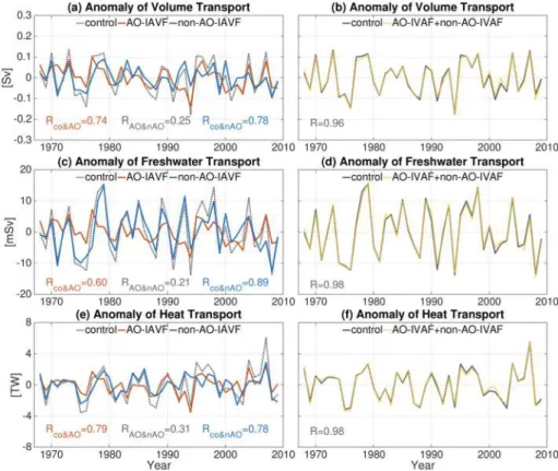
Figure 2.(a) The anomaly of Bering Strait annual mean volume transport in the control experiment (gray dotted line), AO‐IAVF experiment (red solid line), and non‐AO‐IAVF experiment (blue solid line). (b) The anomaly of the volume transport in the control experiment (gray solid line) and the sum of those from AO‐IAVF and non‐AO‐IAVF (yellow dotted line). (c and d) The same as (a) and (b) but for anomalies of freshwater transport. (e and f) The same as (a) and (b) but for anomalies of heat transport. The correlation coefficients between the curves are shown; they are significant at the 0.05 level except for the correlations between the AO‐IAVF and non‐AO‐IAVF runs. The 42‐year (1968–2009) mean values are removed from the time series to compute the anomalies.
10.1029/2019JC015308
Journal of Geophysical Research: Oceans
A historical simulation (hereinafter referred to as“control”) was carried out using the interannually varying forcing (IAVF) of the CORE‐II data sets. Two sensitivity experiments were carried out by using the combi- nation of the IAVF and the normal year forcing (NYF) version of the CORE‐II data sets. The NYF consists of one‐year atmospheric forcing representing the mean climatology of atmosphericfields averaged over the period 1984–2000 (Large & Yeager, 2009). Thefields in the NYF have the same frequencies as in the IAVF. In one sensitivity run we used IAVF inside the Arctic Ocean and NYF outside the Arctic Ocean (here- inafter referred to as“AO‐IAVF”). The Arctic region is defined by the Arctic gateways of the Bering, Davis, and Fram Straits and the Barents Sea Opening (see Figure 1a). In the other sensitivity run we used the NYF in the Arctic Ocean region and the IAVF outside the Arctic Ocean (hereinafter referred to as“non‐AO‐
IAVF”). These two simulations allow us to distinguish the impacts of the atmosphere forcing in the two regions on the interannual variability of the Bering Strait transport. This method to decompose the atmo- spheric forcing geometrically has been successfully employed in a study on the ocean transport variability through the Barents Sea Opening (Wang, Wang, et al., 2019).
All the simulations were carried out for 62 years (1948–2009). The one‐year NYF was applied repeatedly when it was used. Thefirst 20 years are considered as spin‐up and we analyze the last 42 years. To evaluate the control simulation, we used observational data provided by Woodgate et al. (2015) and Woodgate (2018), which is available from http://psc.apl.washington.edu/.
3. Results
The mean volume transport averaged over the last 42 years (1968–2009) is 0.91 Sv in the control run, which is within the range of the climatological values from observations (0.8–1 Sv; Roach et al., 1995; Woodgate, 2018). The anomaly of annual mean volume transport of the control run and in situ observations is shown in Figure 1b. The respective mean volume transport is removed from each time series to obtain the anoma- lies. The observational uncertainty is given as standard errors assuming an appropriate number of degrees of freedom (Woodgate, 2018). For the period of 1998–2009 when continuous observations are available, the cor- relation coefficient between the modeled and observational data is 0.77 (p= 0.01). The observed events of high inflow (2004 and 2007) and low inflow (2001, 2005, and 2008) are well reproduced in the model. In addi- tion, the simulated volume transport interannual variability compares very well with other ocean general circulation models using the same atmospheric forcing analyzed in Wang et al. (2016b) as shown in Figure 1e.
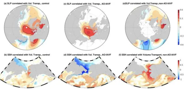
Figure 3.Correlation coefficients between annual mean sea level pressure (SLP) and Bering Strait volume transports in (a) control, (c) AO‐IAVF, and (e) non‐AO‐IAVF runs. Correlation coefficients between annual mean sea surface height (SSH) and Bering Strait volume transports in (b) control, (d) AO‐IAVF, and (f) non‐AO‐IAVF runs. The black contours represent thepvalues of 0.05.
10.1029/2019JC015308
Journal of Geophysical Research: Oceans
The simulated Bering Strait freshwater and heat transports are 65.32 mSv (referenced to 34.8 psu) and 9.7 TW (referenced to−1.9 °C) averaged over the last 42 model years, respectively. They are at the lower bound of the uncertainty ranges suggested by observations and synthesis (2,500 ± 300 km3/year (Woodgate et al., 2005) and 3–6 × 10²⁰J/year (Woodgate et al., 2010)). The observed variation of both the freshwater and heat transports is reasonably reproduced by the control simulation, as shown in Figures 1c and 1d. This is because a large part of the variability of freshwater and heat transports can be attributed to the ocean volume trans- port (Woodgate, 2018; Woodgate et al., 2006), which is well represented in the model.
The Ekman transport through the Bering Strait has much weaker variability than the total ocean volume transport in the control run (an order of magnitude lower; see Figure 1f). Therefore, as expected, the varia- bility of the volume transport can be mainly attributed to changes in the SSH gradient between the Arctic and northern Pacific Oceans. In the following we will use the sensitivity runs to distinguish the variability originating from the two basins.
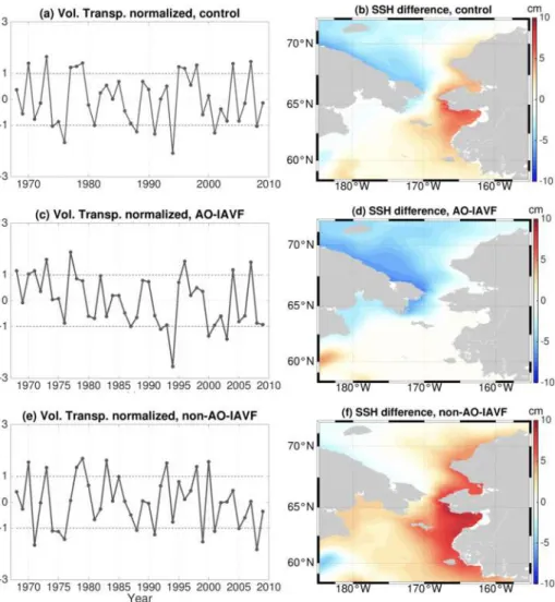
Figure 2a shows the Bering Strait volume transport anomalies for the three simulations. The variances of the volume transport in AO‐IAVF (2.9 × 10⁻³Sv2) and non‐AO‐IAVF (2.8 × 10⁻³Sv2) are very similar, which indicates that the atmospheric forcings inside and outside the Arctic Ocean are equally important for the strength of the interannual variability of the volume transport over the period considered. The correlation Figure 4.(a) The volume transport anomaly normalized by its standard deviation in control run. The black dotted lines indicate the ±1 range for defining years of high and low throughflow in the control experiment. (b) The difference of SSH between years with high and low Bering Strait volume transport (the years are defined as in (a)) in the control run. (c and d) The same as (a) and (b) but for the AO‐IAVF experiment. (e and f) The same as (a) and (b) but for the non‐AO‐IAVF experiment.
10.1029/2019JC015308
Journal of Geophysical Research: Oceans
of the volume transports between the two sensitivity runs is weak (r= 0.25,p= 0.11; Figure 2a), with a covariance of (0.7 × 10⁻³ Sv2). This indicates that the variability of the atmospheric forcing over the Arctic and North Pacific basins, which drives the respective component of the volume transport variability, is by large independent.
It is very interesting to see that summing the volume transport anomalies from the AO‐IAVF and non‐ AO‐IAVF runs well replicates the control run result (Figure 2b; the correlation coefficient is as high as 0.96,p= 0.01). The variance of the volume transport in the control run is 7.2 × 10⁻³Sv2. The sum of the variances in AO‐IAVF and non‐AO‐IAVF and twice of their covariance is 7.1 × 10⁻³Sv2. So the misfit is only about 1% in representing the volume transport variance using the linear combination of the two sensitivity runs. This supports our idea of decomposing the atmospheric forcing geometrically using sen- sitivity runs to quantify the sources of the interannual variability. As shown in Figures 2d and 2f, combin- ing the two sensitivity runs can also well replicate the control run results for both the freshwater and heat transports.
To understand the impact of the atmospheric forcing on the Bering Strait volume transport, we show the cor- relation coefficient of the volume transport with sea level pressure (SLP) and SSH in the top and bottom panels of Figure 3, respectively. In the control run, the volume transport is significantly correlated with the SLP in the Gulf of Alaska and in the Arctic area from the Beaufort Sea to the central Arctic, and antic- orrelated with the SLP along the western coast of the Bering Sea (Figure 3a). The correlation of the volume transport with the SSH is negative along the East Siberian Sea coast and positive along the eastern Bering coast (Figure 3b). The SSH correlation map of the AO‐IAVF run (Figure 3d) also shows negative values along the East Siberian Sea coast, while it reveals a clear signal of fast wave propagation toward the Bering Sea, as proposed in the previous study by Danielson et al. (2014). That is, the variability of SSH over the western Bering Sea shelf is the result of wave propagation from the Arctic Ocean, because only the atmospheric for- cing inside the Arctic Ocean has interannual variability in AO‐IAVF. This signal cannot be directly shown by the correlation between the SSH and ocean volume transport in the control run, because the variability of the volume transport in the control run consists of components induced by the forcing over both sides of the Arctic Ocean.
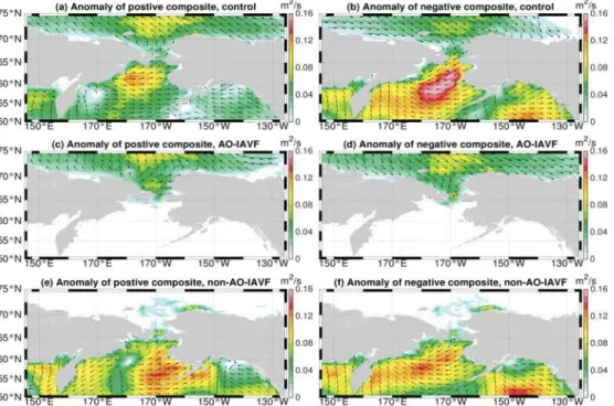
Figure 5.Composite plots of Ekman transport anomalies. (a) The anomaly of Ekman transport for high‐throughflow years (the years are defined as in Figure 4). (b) The same as (a) but for the low‐throughflow years. (c and d) The same as (a) and (b) but for the AO‐IAVF experiment. (e and f) The same as (a) and (b) but for the non‐AO‐IAVF experiment. The color maps represent the magnitude of the Ekman transport and the arrows represent the directions.
10.1029/2019JC015308
Journal of Geophysical Research: Oceans
By using composite plots in the following, we can better understand the processes driving the variability of the Bering Strait throughflow. We select the years when the volume transport is outside the range of ±1 stan- dard deviation to define positive and negative composite years (Figures 4a, 4c, and 4e). The patterns of SSH difference between the positive and nega- tive composite years (Figures 4b, 4d, and 4f) are very similar to the corre- lation patterns shown in Figures 3b, 3d, and 3f. The SSH difference can be explained by considering the wind‐driven Ekman transport. In case the Bering Strait inflow is strong, the nearly meridional winds (Figure S1a) result in an Ekman transport anomaly toward the Alaska coast (Figure 5a), while the winds in the western Arctic lead to an offshore Ekman transport anomaly in the Chukchi and East Siberian Seas (Figure 5a). These Ekman transport anomalies increase the SSH over the eastern Bering shelf and reduce the SSH along the East Siberian Sea coast (Figures 3b and 4b). The increased SSH gradient between the Bering Sea and Arctic Ocean results in stronger Pacific Water inflow to the Arctic Ocean. In case the inflow is weak, the Ekman transport direc- tion is opposite to the case when the inflow is strong (cf. Figures 5a and 5b).
When the inflow is strong in the control run, the Beaufort High is rela- tively strong and the center of the Aleutian Low is over the Aleutian Basin (Figure S2a). On the contrary, when the inflow is weak, the Beaufort High is relatively week and the center of the Aleutian Low is over the Gulf of Alaska (Figure S2b). Danielson et al. (2014) found that the location of the Aleutian Low can influence wind direction in the Bering Sea on weather time scales, thus modifying the direction of Ekman trans- port, the SSH in the Bering Sea, and consequently the inflow through the Figure 7.(a) Anomalies of Ekman pumping velocity and vertical velocity at
20 m averaged in the box defined in Figure 6a obtained from the AO‐IAVF run. The upward velocity is positive. The vertical velocity at 20 m largely follows the variation of the Ekman pumping velocity. (b) The Hovmöller diagram of lateral mean salinity averaged in the box obtained from the AO‐ IAVF run.
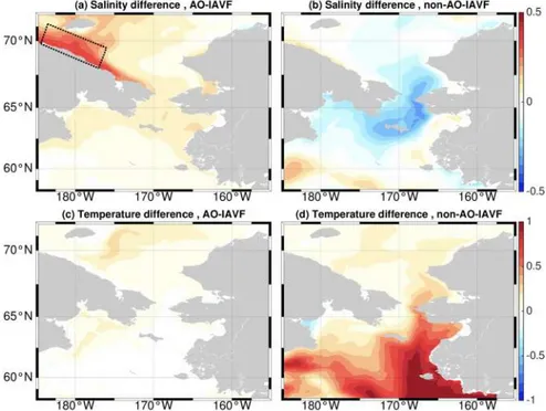
Figure 6.(a) The difference of upper 50‐m mean salinity between years with high and low Bering Strait throughflow (the years are defined as in Figure 4) in the AO‐IAVF run. (b) The same as (a) but for the non‐AO‐IAVF run. (c and d) The same as (a) and (b) but for the temperature difference. Black dotted line marks the box used for calculating averaged salinity, Ekman pumping velocity, and vertical velocity at 20 m shown in Figure 7.
10.1029/2019JC015308
Journal of Geophysical Research: Oceans
Bering Strait. Our results suggest that the location of the Aleutian Low has a similar impact on the Bering Strait inflow on interannual time scales.
Analyzing the two sensitivity runs for the relation of the Bering Strait volume transport with SLP and SSH reveals spatial correlation patterns similar to those obtained from the control run (Figure 3). The directions of the surface Ekman transport anomalies when the Bering Strait volume transport is strong or weak are similar to those in the control run (Figure 5). The correlation between the volume transport and SSH is much higher in the sensitivity runs (Figures 3d and 3f), because the variability of the volume transport is deter- mined by the variation of SSH driven by winds from only one side of the Bering Strait in the two sensitivity runs. This is linked to the fact that the Bering Strait transport variability driven by winds inside and outside the Arctic Ocean is by large not in phase (see Figure 2a). This fact also explains why the composite years are different (Figure 4) and why there are differences in the details of the Ekman transport composites (Figure 5) between the control and sensitivity runs.
The control run alone can provide information that the wind‐driven Ekman transports in both basins can contribute to the variability of the Bering Strait inflow, while the two sensitivity runs can tell which process is exactly responsible for the events of strong and weak inflow obtained in the control run. They reveal that the atmospheric forcing inside and outside the Arctic Ocean do not equally contribute to the outstanding anomalies in the Bering Strait volume transport (Figures 4a, 4c, and 4e). In most of the years when the inflow is lower than 1 standard deviation of the annual mean time series in the control run, the inflow is very weak in both the AO‐IAVF and non‐AO‐IAVF runs. However, in some years with very strong inflow in the control run, the non‐AO‐IAVF run shows relatively low inflow, especially in the 2000s.
We found that the variability of the volume transport induced by the atmospheric forcing over the Arctic Ocean became stronger in recent decades after checking its variance for different periods. The variance of the volume transport in AO‐IAVF is 4.0 × 10⁻³ Sv2 after 1994, about 1.1 × 10⁻³Sv2 higher than the Figure 8.Anomalies of (a and b) ocean volume, (c and d) freshwater, and (e and f) heat transports through the Bering Strait. The left column is for the cases when the interannual variation of atmospheric forcing is kept inside the Arctic Ocean, and the right column is for the cases when the variation of atmospheric forcing is kept outside the Arctic Ocean. In each plot the run with interannual variation only in winds and the run with variation in both winds and buoyancy forcing are compared. All the correlation coefficients shown in the plots are significant at the 0.05 level.
10.1029/2019JC015308
Journal of Geophysical Research: Oceans
variance calculated for the whole period. On the contrary, the variance in non‐AO‐IAVF does not change significantly in recent decades. As a consequence, the correlation of volume transports between the control and AO‐IAVF runs increases from 0.74 (p= 0.01) calculated over the whole period to 0.87 (p= 0.01) over the period after 1994. The enhanced variability of Bering Strait volume transport in AO‐IAVF in recent decades can be explained by stronger variability of winds over the Arctic Ocean. The variance of the wind component along the coastline over the continental shelf of the western Chukchi Sea and East Siberian Sea, corresponding to onshore/offshore Ekman transport, increases from 0.29 m2/s2 over the whole period to 0.42 m2/s2 over 1994–2009, whereas the variance of the wind component along the coastline in the eastern Bering Sea did not change much (slightly reduced) in the recent decades. Our finding is consistent with Peralta‐Ferriz and Woodgate (2017) who suggested that the forcing over the Arctic Ocean plays a predominant role in driving the Bering Strait inflow variability at least since 2002 when the satellite observations became available.
Although the variances of the Bering Strait volume transport in the two sensitivity runs are nearly the same, it is not the case for freshwater and heat transports (Figures 2c and 2e). The variances of the heat transport in the AO‐IAVF and non‐AO‐IAVF runs are 1.38 and 1.80 TW2, respectively, and the variances of the fresh- water transport in these two runs are 12.85 and 41.96 mSv2, respectively. That is, the atmospheric forcing over the North Pacific induces stronger variability for the freshwater and heat transports than the forcing downstream the Bering Strait. The reason is that the salinity and temperature in the inflow water can be influenced by the atmospheric forcing (Figure 6). In comparison to southwestward Ekman transport, north- eastward Ekman transport in the Bering Sea facilitates the accumulation of low‐salinity and high‐ temperature water upstream the Bering Strait (Figures 6b and 6d), because the incoming surface water has the characteristics of low salinity and high temperature (Roach et al., 1995). This strengthens the inter- annual variability of freshwater and heat transports. Even in the period after 1994 when the winds inside the Arctic Ocean have increasing contribution to the volume transport variability, the winds outside the Arctic Ocean retain their significant contribution to the variability of heat and freshwater transports (Figures 2c and 2e), because they cause variations also in the temperature and salinity of the inflow water. As the varia- bility of the freshwater transport in non‐AO‐IAVF is much stronger than in AO‐IAVF, the variability in the Figure 9.The same as Figure 6 but for the runs with interannual variation only in momentum forcing (winds). (a) The difference of salinity between years with high and low Bering Strait throughflow (the years are defined as in Figure 4) in the AO‐IAVF‐w run. (b) The same as (a) but for the non‐AO‐IAVF‐w run. (c and d) The same as (a) and (b) but for the temperature difference.
10.1029/2019JC015308
Journal of Geophysical Research: Oceans
control run (the sum of the two sensitivity runs) is dominated by the variability originating from outside the Arctic Ocean. Consequently, the correlation of the control run with the non‐AO‐IAVF run for the freshwater transport is stronger than with the AO‐IAVF run (Figure 2c).
In AO‐IAVF the salinity along the coast of the East Siberian and Chukchi Seas is higher when the Bering Strait inflow is higher (Figure 6a). Figure 7 shows clear correlation between vertical Ekman pumping velo- city and the ocean salinity in this region. That is, in years when the Bering Strait inflow is high, the Ekman transport is predominantly offshore in the East Siberian Sea and western Chukchi Sea (Figure 5c), which causes upwelling over the continental shelves, thus increasing the upper ocean salinity there.
The above discussions assume that winds are the main driver of the inflow variability. To identify whether the variability of atmospheric buoyancy (heat and freshwater) forcing has significant impacts on the Bering Strait inflow, we repeated the AO‐IAVF and non‐AO‐IAVF simulations in which the climatological heat and freshwater forcing is applied on the global ocean surface (called AO‐IAVF‐w and non‐AO‐IAVF‐w, respec- tively). That is, only wind forcing has interannual variation in these runs (either inside or outside the Arctic Ocean). We found that not only the interannual variability of the Bering Strait volume transport, but also that of heat and freshwater transport, is not very significantly changed by buoyancy forcing (Figure 8).
Therefore, the variation in winds is indeed a key factor determining the interannual variability of the Bering Strait inflow. The heat transport is relatively more sensitive to the buoyancy forcing outside the Arctic Ocean than the ocean volume and freshwater transports (Figure 8f), because the inflow water tem- perature is more sensitive to the thermal forcing (cf. Figures 6 and 9).
4. Discussions and Conclusions
Due to the potential impact of the Bering Strait inflow on Arctic freshwater, sea ice cover, ecosystem, and the large‐scale ocean circulation, a better understanding of the response of the inflow to changes in atmospheric Figure 10.Conceptual diagrams representing the forcing processes driving the interannual variability of the Bering Strait volume transport: the (top) western Arctic and (bottom) northern Pacific. The color maps represent the anomalies of the SLP composites for years with high and low Bering Strait throughflow (the years are defined in Figure 4). The blue arrows represent the directions of winds anomalies and the orange arrows represent the directions of Ekman transport anomalies.
10.1029/2019JC015308
Journal of Geophysical Research: Oceans
forcing is required. In this study, numerical simulations were used to attribute the interannual variability of the Bering Strait inflow to atmospheric forcing in different regions. We kept the interannual variation of the atmospheric forcing only inside or outside the Arctic Ocean in two sensitivity simulations. Summing the anomalies of the Bering Strait inflow from these simulations can very well replicate that from the hindcast control simulation, which facilitated us to quantity forcing processes responsible for the variability of the throughflow.
Our results indicate that the SSH gradient between the Bering Sea and Arctic Ocean drives the variability of the Bering Strait inflow, consistent with previous studies (Coachman & Aagaard, 1988). As shown in the conceptual diagram (Figure 10), the wind‐driven Ekman transport can explain the variation of the SSH on both sides of the Bering Strait (Danielson et al., 2014; Peralta‐Ferriz & Woodgate, 2017). In the Arctic Ocean, changes in the atmospheric circulation associated with the changes in the strength of the Beaufort High can alter the direction of Ekman transport in the Chukchi and East Siberian Seas (Figures 10a and 10b). When the Beaufort High is strong (weak), the Ekman transport is offshore (onshore) in these shelf seas, thus lowering (increasing) the SSH along their coast and increasing (reducing) the Bering Strait inflow. On the Pacific side, the location of the Aleutian Low active center regulates the intensity of the Bering Strait transport. When the center of the Aleutian Low is located over the Aleutian Basin, the Ekman transport diverges over the basin and causes the SSH on the eastern Bering Sea shelf to rise (Figure 10c). This increases the Bering Strait inflow. Conversely, when the active center of the Aleutian Low moves eastward to the Gulf of Alaska, the northeasterly winds prevail on the eastern Bering shelf, which leads to offshore Ekman trans- port on the eastern Bering shelf (Figure 10d). This reduces the SSH there and weakens the Bering Strait inflow. Our model results show that these forcing processes can explain the variability of the Bering Strait inflow on interannual time scales. Here we note that the SSH gradient between the Bering Sea and Arctic Ocean appears as west‐east gradient at the Bering Strait due to Coriolis force. That is, it is the manifestation of the fact that the Bering Strait inflow is predominantly a geostrophicflow.
By decomposing the atmospheric forcing variability geometrically and isolating the forcing components in different sensitivity experiments, we can draw the following conclusions:
1. The interannual variability of the Bering Strait inflow is predominantly induced by momentum forcing (wind) variability. The ocean surface buoyancy forcing (the surface heat and freshwaterfluxes) plays a relatively small role.
2. Considering the past few decades (1968–2009), winds inside the Arctic Ocean and over the North Pacific quantitatively have similar contributions to the variance of the annual mean volume transport through the Bering Strait.
3. The Bering Strait inflow variabilities driven by the winds inside the Arctic Ocean and over the North Pacific are not in phase by large. These winds do not have equal contributions to the extreme anomalies of the Bering Strait volume transport.
4. The wind forcing over the northern Pacific can also change the temperature and salinity of the inflow water by altering the ocean circulation. That is, winds outside the Arctic Ocean influence the variability of Bering Strait heat and freshwater transports not only by changing ocean volume transport through modulating the SSH but also by changing the temperature and salinity of the inflow water through alter- ing the ocean circulation in the Bering Sea. Therefore, winds south of the Bering Strait explain a larger part of the Bering Strait freshwater and heat transport variability than the winds inside the Arctic Ocean.
5. The wind forcing inside the Arctic Ocean has a larger contribution to the variability of the Bering Strait volume transport than that outside the Arctic Ocean after 1994, because the variability of winds on the Arctic side has become stronger in recent decades. This is consistent to thefinding based on satellite observations by Peralta‐Ferriz and Woodgate (2017). However, because winds south of the Bering Strait can impact the heat and freshwater transports through the Bering Strait by changing the tempera- ture and salinity of the inflow water, they still contribute significantly to the variability of heat and fresh- water transports after 1994, although their contribution to the volume transport variability becomes smaller than that provided by the winds inside the Arctic Ocean in this period.
As the interannual variability of the Bering Strait volume transport is closely linked to the SLP, we also want to know whether we can use large‐scale atmospheric circulation indices to directly explain the volume trans- port variability. The correlation coefficients between the volume transport in the AO‐IAVF run and the
10.1029/2019JC015308
Journal of Geophysical Research: Oceans
Arctic Oscillation index (Thompson & Wallace, 1998) and Dipole Anomaly index (Wang et al., 2009; Wu et al., 2006) are only 0.23 (p= 0.15) and−0.13 (p= 0.42), respectively. The volume transport in the non‐
AO‐IAVF run also does not significantly correlate with the North Pacific (r= 0.27, p = 0.08), Pacific North American Pattern (r=−0.22, p= 0.16), North Pacific Oscillation (r= 0.17,p= 0.2), and North Pacific Gyre Oscillation (r = 0.3,p= 0.05) indices (Di Lorenzo et al., 2008; Rogers, 1981; Trenberth &
Hurrell, 1994; Walker & Bliss, 1932). Therefore, the details in local winds in the western Arctic Ocean and in the northern North Pacific are important in modulating the transport variability.
In this paper we used a well‐developed medium‐resolution model setup with the CORE‐II atmospheric for- cing to understand and quantify the origin of the interannual variability of the Bering Strait inflow. In future work we will develop a new model setup using forcing data sets updated to recent years in order to under- stand the changes of the Bering Strait inflow observed in the recent decade.
References
Aagaard, K., & Carmack, E. C. (1989). The role of sea ice and other fresh water in the Arctic circulation.Journal of Geophysical Research, 94(C10), 14,485–14,498.
Aagaard, K., Coachman, L. K., & Carmack, E. (1981). On the halocline of the Arctic Ocean. Deep Sea Research Part A.Oceanographic Research Papers,28(6), 529–545.
Aagaard, K., Weingartner, T. J., Danielson, S. L., Woodgate, R. A., Johnson, G. C., & Whitledge, T. E. (2006). Some controls onflow and salinity in Bering Strait.Geophysical Research Letters,33, L19602. https://doi.org/10.1029/2006GL026612
Coachman, L. K., & Aagaard, K. (1966). On the water exchange through Bering Strait 1.Limnology and Oceanography,11(1), 44–59.
Coachman, L. K., & Aagaard, K. (1988). Transports through Bering Strait: Annual and interannual variability.Journal of Geophysical Research,93(C12), 15,535–15,539.
Dai, A., Qian, T., Trenberth, K. E., & Milliman, J. D. (2009). Changes in continental freshwater discharge from 1948 to 2004.Journal of Climate,22(10), 2773–2792.
Danielson, S. L., Weingartner, T. J., Hedstrom, K. S., Aagaard, K., Woodgate, R., Curchitser, E., & Stabeno, P. J. (2014). Coupled wind‐ forced controls of the Bering–Chukchi shelf circulation and the Bering Strait throughflow: Ekman transport, continental shelf waves, and variations of the Pacific–Arctic sea surface height gradient.Progress in Oceanography,125, 40–61.
Danilov, S., Wang, Q., Timmermann, R., Iakovlev, N., Sidorenko, D., Kimmritz, M., et al. (2015). Finite‐element sea ice model (FESIM), version 2.Geoscientific Model Development,8(6), 1747–1761.
Di Lorenzo, E., Schneider, N., Cobb, K. M., Franks, P. J. S., Chhak, K., Miller, A. J., et al. (2008). North Pacific Gyre Oscillation links ocean climate and ecosystem change.Geophysical Research Letters,35, L08607. https://doi.org/10.1029/2007GL032838
Goosse, H., Campin, J. M., Fichefet, T., & Deleersnijder, E. (1997). Sensitivity of a global ice–ocean model to the Bering Strait throughflow.
Climate Dynamics,13(5), 349–358.
Hu, A., Meehl, G. A., & Han, W. (2007). Role of the Bering Strait in the thermohaline circulation and abrupt climate change.Geophysical Research Letters,34, L05704. https://doi.org/10.1029/2006GL028906
Hu, A., Meehl, G. A., Otto‐Bliesner, B. L., Waelbroeck, C., Han, W., Loutre, M. F., et al. (2010). Influence of Bering Straitflow and North Atlantic circulation on glacial sea‐level changes.Nature Geoscience,3(2), 118.
Ilıcak, M., Drange, H., Wang, Q., Gerdes, R., Aksenov, Y., Bailey, D., et al. (2016). An assessment of the Arctic Ocean in a suite of inter- annual CORE‐II simulations. Part III: Hydrography andfluxes.Ocean Modelling,100, 141–161.
Large, W. G., & Yeager, S. G. (2009). The global climatology of an interannually varying air–seaflux data set.Climate Dynamics,33(2‐3), 341–364.
Peralta‐Ferriz, C., & Woodgate, R. A. (2017). The dominant role of the East Siberian Sea in driving the oceanicflow through the Bering Strait—Conclusions from GRACE ocean mass satellite data and in situ mooring observations between 2002 and 2016.Geophysical Research Letters,44(22), 11,472–11,481. https://doi.org/10.1002/2017GL075179
Roach, A. T., Aagaard, K., Pease, C. H., Salo, S. A., Weingartner, T., Pavlov, V., & Kulakov, M. (1995). Direct measurements of transport and water properties through the Bering Strait.Journal of Geophysical Research,100(C9), 18,443–18,457.
Rogers, J. C. (1981). The North Pacific oscillation.Journal of Climatology,1(1), 39–57.
Serreze, M. C., Barrett, A. P., Slater, A. G., Woodgate, R. A., Aagaard, K., Lammers, R. B., et al. (2006). The large‐scale freshwater cycle of the Arctic.Journal of Geophysical Research,111, C11010. https://doi.org/10.1029/2005JC003424
Shaffer, G., & Bendtsen, J. (1994). Role of the Bering Strait in controlling North Atlantic Ocean circulation and climate.Nature,367(6461), 354.
Springer, A. M., & McRoY, C. P. (1993). The paradox of pelagic food webs in the northern Bering Sea—III. Patterns of primary production.
Continental Shelf Research,13(5‐6), 575–599.
Steele, M., Morley, R., & Ermold, W. (2001). PHC: A global ocean hydrography with a high‐quality Arctic Ocean.Journal of Climate,14(9), 2079–2087.
Thompson, D. W., & Wallace, J. M. (1998). The Arctic Oscillation signature in the wintertime geopotential height and temperaturefields.
Geophysical Research Letters,25(9), 1297–1300.
Torres‐Valdés, S., Tsubouchi, T., Bacon, S., Naveira‐Garabato, A. C., Sanders, R., McLaughlin, F. A., et al. (2013). Export of nutrients from the Arctic Ocean.Journal of Geophysical Research, Oceans,118(4), 1625–1644. https://doi.org/10.1002/jgrc.20063
Trenberth, K. E., & Hurrell, J. W. (1994). Decadal atmosphere‐ocean variations in the Pacific.Climate Dynamics,9(6), 303–319.
Tseng, Y. H., Lin, H., Chen, H. C., Thompson, K., Bentsen, M., Böning, C. W., et al. (2016). North and equatorial Pacific Ocean circulation in the CORE‐II hindcast simulations.Ocean Modelling,104, 143–170. https://doi.org/10.1016/j.ocemod.2016.06.003
Walker, G. T., & Bliss, E. W. (1932).World Weather V,Memories of the Royal Meteorological Society(Vol. 4, pp. 53–84). London: Edward Stanford.
Wang, J., Zhang, J., Watanabe, E., Ikeda, M., Mizobata, K., Walsh, J. E., et al. (2009). Is the Dipole Anomaly a major driver to record lows in Arctic summer sea ice extent?Geophysical Research Letters,36, L05706. https://doi.org/10.1029/2008GL036706
10.1029/2019JC015308
Journal of Geophysical Research: Oceans
Acknowledgments
W. Zhang and X. Wang are supported by the National Key R&D Program of China (grant 2016YFC1401507), National Natural Science Foundation of China (grant 41806218), the Fundamental Research Funds for the Central Universities (grant 2017B04414), and Natural Science Foundation of Jiangsu Province (grant BK20180510). W. Zhang is supported in part by the scholarship from China Scholarship Council (CSC) under grant CSC 201806710104. Q. Wang is sup- ported by the Helmholtz Climate Initiative REKLIM (Regional Climate Change). We thank the two reviewers for their helpful comments. The obser- vational data of ocean volume, fresh- water, and heat transports through Bering Strait used in this paper were obtained from http://psc.apl.washing- ton.edu/HLD/Bstrait/Data/
BeringStraitMooringDataArchive.html.
The model results used in this paper are stored at https://doi.org/10.5281/
zenodo.2648156.
Wang, Q., Danilov, S., Sidorenko, D., Timmermann, R., Wekerle, C., Wang, X., et al. (2014). The Finite Element Sea Ice‐Ocean Model (FESOM) v. 1.4: Formulation of an ocean general circulation model.Geoscientific Model Development,7(2), 663–693. https://doi.org/
10.5194/gmd‐7‐663‐2014
Wang, Q., Ilicak, M., Gerdes, R., Drange, H., Aksenov, Y., Bailey, D. A., et al. (2016a). An assessment of the Arctic Ocean in a suite of interannual CORE‐II simulations. Part I: Sea ice and solid freshwater.Ocean Modelling,99, 110–132. https://doi.org/10.1016/j.
ocemod.2015.12.008
Wang, Q., Ilicak, M., Gerdes, R., Drange, H., Aksenov, Y., Bailey, D. A., et al. (2016b). An assessment of the Arctic Ocean in a suite of interannual CORE‐II simulations. Part II: Liquid freshwater.Ocean Modelling,99, 86–109.
Wang, Q., Marshall, J., Scott, J., Meneghello, G., Danilov, S., & Jung, T. (2019). On the feedback of ice‐ocean stress coupling from geos- trophic currents in an anticyclonic wind regime over the Beaufort Gyre.Journal of Physical Oceanography,49, 369–383.
Wang, Q., Wang, X., Wekerle, C., Danilov, S., Jung, T., Koldunov, N., et al. (2019). Ocean heat transport into the Barents Sea: Distinct controls on the upward trend and interannual variability.Geophysical Research Letters,46(22), 13180–13190. https://doi.org/10.1029/
2019GL083837
Woodgate, R. A. (2018). Increases in the Pacific inflow to the Arctic from 1990 to 2015, and insights into seasonal trends and driving mechanisms from year‐round Bering Strait mooring data.Progress in Oceanography,160, 124–154.
Woodgate, R. A., Aagaard, K., & Weingartner, T. J. (2005). Monthly temperature, salinity, and transport variability of the Bering Strait throughflow.Geophysical Research Letters,32, L04601. https://doi.org/10.1029/2004GL021880
Woodgate, R. A., Aagaard, K., & Weingartner, T. J. (2006). Interannual changes in the Bering Straitfluxes of volume, heat and freshwater between 1991 and 2004.Geophysical Research Letters,33, L15609. https://doi.org/10.1029/2006GL026931
Woodgate, R. A., Stafford, K. M., & Prahl, F. G. (2015). A synthesis of year‐round interdisciplinary mooring measurements in the Bering Strait (1990–2014) and the RUSALCA years (2004–2011).Oceanography,28(3), 46–67.
Woodgate, R. A., Weingartner, T., & Lindsay, R. (2010). The 2007 Bering Strait oceanic heatflux and anomalous Arctic sea‐ice retreat.
Geophysical Research Letters,37, L01602. https://doi.org/10.1029/2009GL041621
Woodgate, R. A., Weingartner, T. J., & Lindsay, R. (2012). Observed increases in Bering Strait oceanicfluxes from the Pacific to the Arctic from 2001 to 2011 and their impacts on the Arctic Ocean water column.Geophysical Research Letters,39, L24603. https://doi.org/
10.1029/2012GL054092
Wu, B., Wang, J., & Walsh, J. E. (2006). Dipole Anomaly in the winter Arctic atmosphere and its association with Arctic sea ice motion.
Journal of Climate,19, 210–225.
10.1029/2019JC015308