Difference in soil parameters between disturbed and undisturbed permafrost soil in Northwest Territories,

(1)

Difference in soil parameters between disturbed and undisturbed permafrost soil in Northwest Territories,

Canada

A thesis presented for the degree of Bachelor of Science at

Institute of Environmental Science and Geography University of Potsdam

Germany

Frieder Tautz Pr¨asidentenstr. 73 16816 Neuruppin Matrikel-Nr.: 780602

frtautz@uni-potsdam.de Potsdam, October 12, 2020

(2)

1st supervisor Prof. Dr. Guido Grosse

Alfred-Wegener-Institut, Polar- und Meeresforschung Telegrafenberg A45-N, 14473 Potsdam

2nd supervisor Prof. Dr. Julia Boike

Alfred-Wegener-Institut, Polar- und Meeresforschung Telegrafenberg A6, 14473 Potsdam

(3)

List of Figures

1 Permafrost carbon cycle (Schuur et al. 2015) . . . 4

2 Schematic of retrogressive thaw slumps (Lantuit and Pollard 2005) . . . 7

3 Schematic of a non-sorted soil profile (Margesin 2009) . . . 9

4 Physiographic subdivision and overview map of study sites . . . 11

5 Examples of sites categorised as disturbed at Lake 6 . . . 13

6 High vegetation at disturbed sites at Lake 6 . . . 14

7 Examples of sites defined as undisturbed . . . 14

8 First pit after drilling the first core at Lake 1 . . . 15

9 Coring equipment . . . 16

10 Sampling setup in-situ . . . 17

11 Cylinder and AL soil samples taken at TVC and Lake 11 respectively . . . 17

12 Core obtained at Lake 1 in cooling chamber, AWI . . . 18

13 Subsampling for different analyses in cooling chamber . . . 19

14 Setup of Rhizon soil moisture sampling, AWI Potsdam . . . 21

15 Cryotic processes visible in soil profiles . . . 25

16 Comparison between AL and permafrost of biochemical values and CN-ratio . . . 29

17 Grain size differentiation over the three depth categories of AL measurements . . . 30

18 ALT measurements of disturbed and undisturbed sites . . . 31

19 Difference between disturbed and undisturbed sites of biochemical parameters . . . 32

20 Grain size distribution . . . 33

21 Weight percentage of grains larger than 1 mm not included in the grain size analysis . . . 41

A1 General temperature regime of permafrost (French 2013) . . . . 55 A2 Map of sampling setup at Lake 1 regarding the main data set . 62 A3 Map of sampling setup at Lake 6 regarding the main data set . 62 A4 Map of sampling setup at Lake 11 regarding the main data set . 63

(6)

A5 Map of sampling setup at TVC and 1sub3 regarding the main

data set . . . 63

A6 Map of sampling setup at Lake 12 regarding the main data set . 64 A7 Map of sampling setup at Lake 1 regarding the extended data set with ALT measurements . . . 64

A8 Map of sampling setup at Lake 6 regarding the extended data set with ALT measurements . . . 65

A11 Map of sampling setup of vegetation sites regarding the extended data set with ALT measurements . . . 66

List of Tables

1 Rate of mineralisation in regard to TOC/TN-ratio (Walthert et al. 2004) . . . 5

2 Radiocarbon age at different sites . . . 26

3 Summary of additional measurements - gravimetric and volumetric ice content, wet and dry bulk densities . . . 27

4 SOCC values at each sample site . . . 32

A1 Biochemical parameters of permafrost core and active layer samples . . . 55

A1 Grain size distribution . . . 57

A1 Excluded grain fraction>1mm . . . 59

A1 Extended data set with ALT measurements . . . 60

(7)

Acronyms

CH₃COOH Acetic acid is a colourless organic acid with the formular CH₃COOH.

CH₄ Methane is an organic gas with the formula CH₄. It is utilised as a fuel and forms naturally below ground and under the seafloor by biological and geological processes. In the atmosphere, it plays an important role as a Greenhouse Gas.

CO₂ Carbon dioxide is a colourless gas with the formula CO₂, naturally occurring in the atmosphere and hydrosphere. It plays a major role as a Greenhouse Gas in the atmosphere where it stores thermal energy and enhances global warming.

H₂O₂ Hydrogen peroxide is a chemical compound used as an oxidiser, bleaching agent and antiseptic.

N₂O Nitrous oxide, also known as laughing gas, is a chemical molecule with the formula N₂O. It is commonly used as an anaesthetic in health system. In the atmosphere, it acts as a Greenhouse Gas

12C The carbon-12 isotope is the most abundant isotope of carbon and makes roughly 98% of the carbon on earth. Its amount in organics is used to determine its age with the Radiocarbon dating method.

13C The carbon-13 isotope is one of the three carbon isotope, is quite stable and makes roughly 1 % of the naturally occurring carbon on earth.

14C The carbon-14 isotope is quite unstable and the rarest of all three carbon isotopes. Its occurrence and decay in organic materials is the basis of the Radiocarbon dating method utilised to determine the age of organics.

14N The nitrogen-14 isotope is the major isotope of nitrogen.

m³ 1 cubic metre = 1m∗1m∗1m.

°C Degree Celsius is a common unit to describe temperature. Zero degree celsius are 32 Fahreneinheit or 273,15 Kelvin.

14C Radiocarbon dating is method utilising the decay of the ₁₄C isotope to determine the age of organic materials for example in soils.

a years

AL The Active layer is the top soil layer in permafrost areas. It freezes in winter and thaws in summer due to seasonal changes.

ALT The Active Layer Thickness is the average annual thaw depth of the acitve layer.

AMS The Accelerator Mass Spectrometer is a sensitive device measuring the amount and type of isotopes in a probe. Its major use is to determine Radiocarbon date by measuring the amount of the according isotopes.

(8)

AWI Alfred-Wegener-Institut, Helmholtz-Zentrum for Polar and Marine Research

C Carbon is a chemical element and the main component of all organics on earth.

C/N ratio The Total Organic Carbon to Total Nitrogen ration describes the proportion between those two soil components and is often utilised to indicate the rate of mineralisation in the soil (Walthert et al. 2004).

cal. a BP Calibrated radiocarbon years before present refer to the cor- rected age calculation of organic material with the Radiocarbon dating method. Due to different concentrations in the past, the age calculations requires adjustment according to the historic isotope concentrations in the atmosphere.

cm 1 centimetre = 1∗10^–2 m

DZAA The Depth of Zero Annual Amplitude describes the depth in permafrost soils where there is no annual fluctuations by seasonal changes (<0.1 degree celsius (°C)). It is utilised to determine long-term changes of the permafrost temperature.

g Gram is the SI-unit for weight.

GHG Greenhouse Gases are radioactive gases in the thermal infrared spectrum rising global temperatures with rising concentrations in the atmosphere. This process is termed Greenhouse Effect.

GSD The Grain Size Distribution describes the size and relative amount of grains in a probe by mass or volume. It determines the soil class, the soils composition and movement of water.

ka Thousand years

kg 1 kilogram = 10 g

kg/m² kilograms per square metre

km 1 kilometre = 1000 m

km² 1 square kilometre = 1km∗1km m metre (SI-unit of length)

m² 1 square metre = 1m∗1m

m/a metre per year

mg 1 Milligram = 10^–3 metre

mineralisation Mineralisation is the process of complete decomposition of organic material to inorganic components - mainly by microor- ganisms activity. It releases primarily photosynthetically sequestered carbon as carbon dioxide as well as other components of the cycle of matter such as nitrogen, phosphor or sulphur.

ml 1 millilitre = 10^–3 litre.

mm 1 Millimetre = 10^–3 metre

N Nitrogen is a chemical element with the formula N. In soils it is often the limiting nutrient for plants.

North The decimal latitudinal degrees is a unit to describe a position on earth. Together with the longitudinal degrees, each position on the surface can be assigned to a unique combination of Latitudes and Longitudes. Due to the fact that latitudinal degrees are describing the angle towards the equator, they are devided by their position relative to the equator into north and south.

(9)

NWT The Northwestern Territories is a state north-west in Canada.

OM Organic Matter is the carbon-based component of a sample which derives from living organisms such as plants, animals and microbes.

Pg 1 Pg = 10¹⁵ g

RCP The Representatiive Concentration Pathway describes the trajectory of Greenhouse Gases (GHG) concentration in the atmosphere in the future and is utilised for modeling and research purposes. The concentrations are highly dependent on the emissions by human kind.

SOCC The Soil Organic Carbon Content is an important parameter describing the amount of organic carbon in the soil with the unit [kg/m²]. It always refers to a certain soil depth - f.e. the first metre of the soil, and is integrated over the whole column.

TC Total Carbon is the amount of carbon in a sample as a fraction in regard to its total weight or volume (unit: [wt% or vol%]).

Major sources are organic material from living organisms, car- bonates and dissolved CO₂.

TN The Total Nitrogen content refers to the amount of Nitrogen in a sample by weight or volume in [wt%] or [vol%].

TOC Total Organic Carbon is the fraction of all carbon originated from living organisms divided by the total amount of the sample. The unit is either in percentage by weight [wt%] or volume [vol%].

TVC The Trail Valley Creek camp side is a research facility of the Wilfried Lauries University 50 km north of Inuvik, Canada. In this thesis it is also sampling site.

vol% Volumetric percentage describes the relative amount of a component by volume.

West The decimal longitudinal degrees is a unit to describe a position on earth. Together with the latitudinal degrees, each position on the surface can be assigned to one unique combination of Latitudes and Longitudes. Due to the fact that longitudinal degrees are described according to their angle towards prime meridian, they are divided by their position relative to the prime meridian into east and west.

wt% Gravimetric percentage describes the relative amount of a component by mass.

(10)

Abstract

As a result of strong climatic changes in arctic regions, permafrost areas are subject to substantial modifications. The matter raises global concerns due to the permafrost carbon climate feedback causing large amounts of Greenhouse Gases to be released into the atmosphere. Ris- ing temperatures and climatic changes lead to permafrost disturbances developing distinct features termed thermokarsts.

Thermokarsts evolve when ice-rich permafrost thaws and the soil collapses into the volume previously occupied by ice. In this study, the main focus lies on the thermokarst feature retrogressive thaw slump in the proximity of lakes. The differences in soil parameters between the Active Layer and permafrost and between disturbed and undisturbed permafrost ground are examined to give indications about the paramet- rical changes of permafrost soils in respect to climate change, permafrost disturbance and the consequent development of thermokarsts. Carbon, nitrogen, grain size, ice content and Radiocarbon dating analysis were conducted for this thesis.

Carbon and Nitrogen are clearly depleted in the active layer compared to values in the cryotic ground and in disturbed compared to undisturbed ground. Further detailed analyses between sites reveal highly fluctu- ating dynamics and suggest that permafrost disturbance, thermokarst development and hence the release of Greenhouse Gases strongly de- pends on site-specific features such as vegetation cover, orientation, slope angle, water content and the local landscape history. Although thermokarsts and Greenhouse Gas release are known to increase in the future, how and to what extent controlling factors influence the soils development on a local scale is yet to be determined.

(11)

Zusammenfassung

Infolge der starken Ausprägung globaler Erwärmung in arktischen Regionen sind elementare Veränderung in den Permafrostgebieten zu erwarten. Durch die positive Rückkopplung des Permafrostkohlenstoffs auf den Klimawandel, werden große Mengen von Treibhausgasen in die Atmosphäre freigesetzt. Steigende Temperaturen und veränderte klima- tische Bedingungen führen zu Permafroststörungen mit ausgeprägten Landschaftsmerkmalen - genannt Thermokarsts.

Thermokarsts entstehen, wenn eisreicher Permafrost auftaut und der Boden in das zuvor vom Eis eingenommene Volumen kollabiert. In dieser Studie liegt der Fokus auf Thermokarsts mit rückläufigen Hangrutschun- gen (retrogressive thaw slumps) in der Nähe von Seen. Die Unterschiede in den Bodenparametern zwischen der aktiven Schicht und dem Per- mafrost, sowie zwischen gestörtem und ungestörtem Permafrostboden werden untersucht, um Hinweise auf die parametrischen Veränderungen der Permafrostböden in Bezug auf Klimaänderung, Permafroststörung und die daraus resultierende Entwicklung von Thermokarsts zu geben.

Für diese Arbeit wurden Kohlenstoff-, Stickstoff-, Korngrössen-, Eisgehalts- und Radiokarbon-Datierungsanalysen durchgeführt.

Kohlenstoff und Stickstoff sind in der aktiven Schicht im Vergleich zu Werten im kryotischen Boden deutlich niedriger. Das gleiche gilt auch für Kohlenstoff und Stickstoff in gestörtem im Vergleich zu ungestörtem Boden. Weitere detaillierte Analysen zwischen den Standorten zeigen eine stark schwankende Dynamik und legen nahe, dass Permafroststörung, Thermokarstentwicklung und damit die Freisetzung von Treibhausgasen stark von standortspezifischen Merkmalen wie Vegetationsbedeckung, Orientierung, Hangneigung, Wassergehalt und der lokalen Landschafts- geschichte abhängt. Obwohl bekannt ist, dass die Thermokarstbildung und die Freisetzung von Treibhausgasen in Zukunft zunehmen werden, ist noch nicht geklärt, wie und in welchem Umfang steuernde Faktoren die Entwicklung der Böden auf lokaler Ebene beeinflussen.

(12)

1 Introduction

Permafrost areas contain vast amounts of Organic Matter (OM) sequestered over millennia in the soil (Hugelius et al. 2014a,b; Kutzbach et al. 2010; Schuur et al. 2015; Tamocai et al. 2009). As a result of climate change, permafrost areas get disturbed and thermokarst terrain develops and enlarges. When permafrost thaws, previously sequestered Carbon (C) is decomposed by increased microbial activity releasing GHG into the atmosphere (Burn 2011; Everdin- gen 1998; Grosse et al. 2011; Kokelj and Jorgenson 2013; Kokelj et al. 2009;

Marushchak et al. 2011; McGuire et al. 2009; Repo et al. 2009; Romanovsky et al. 2017; Schaefer et al. 2011; Tamocai et al. 2009; Turetsky et al. 2019; Vardy et al. 2000). A changing landscape poses serious threats to settlements in regions with permafrost occurrence and its positive feedback to climate change rises global concerns.

The aim of the thesis is to connect certain soil properties with the degradation of permafrost, in particular at retrogressive thaw slumps. With the aid of several soil parameters, conclusions may be drawn regarding the nature of landscape modifications in arctic regions. The following hypotheses will be investigated:

I. General properties (ice content, active layer thickness (ALT), bulk densities and radiocarbon dating (14C) measurements) are expected to reflect typical characteristics of permafrost soils in the Northwestern Territories (NWT), Canada (Burn and Michel 1988; Kokelj and Burn 2003, 2005;

Kokelj et al. 2002; Lacelle et al. 2004; Mackay 1983; Ping et al. 2008;

Tarnocai and Bockheim 2011).

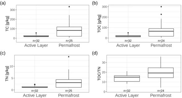
II. Biochemical compounds (Total Organic Carbon (TOC),Total Carbon (TC) and Total Nitrogen (TN)) are expected to be depleted in the active layer (AL) indicating higher (mineralisation) rates compared to the cryotic ground (Broll et al. 1999; Pries et al. 2012; Schuur et al. 2015; Sollins et al. 1984; Stevenson 1994; Strauss 2010; Vardy et al. 2000; Walthert et al. 2004). The grain size distribution (GSD) may show translocation dynamics in finer grain fractions (Broll et al. 1999; Kokelj and Burn 2003;

Locke 1986; Tarnocai and Bockheim 2011)

III. Comparison between disturbed and undisturbed categorised sites is con- sulted to reveal processes within soil profiles connected to thermokarst development, thawing of permafrost and deepening ALT. At disturbed sites, increasing temperatures may result in deeper ALT with increasing mineralisation rates exhibiting lower C and TN contents and narrower Total Organic Carbon to Total Nitrogen ratio (C/N ratio) (Brouchkov

(13)

et al. 2004; Burn 1997; Lacelle et al. 2010; Lantz et al. 2009; Nixon and Taylor 1998; Strauss 2010; Vardy et al. 1998).

1.1 Scientific background

1.1.1 Permafrost distribution and properties

Permafrost is defined as ground material containing ice and organic materials which exhibits a temperature regime lower than 0 °C for at least two consecutive years (Brown and Kupsch 1974; Everdingen 1998). The development of terrestrial permafrost (exclusively referred to in this thesis) is mainly controlled by prevailing climatic conditions but also by the historic landscape evolution and the altitude of the landscape. That is why permafrost can occur around the globe to differing extents.

Globally, 16 – 21∗10⁶ square kilometres (km²) of the exposed land surface is estimated to exhibit permafrost conditions (Gruber 2012). This accounts for 12.4-16.3 % of the exposed land surface. Permafrost occurs in higher quantities on the northern hemisphere (13– 18∗10⁶ km² north of 60 degrees South) due to its larger land surface area (Gruber 2012). Its thickness can range from a few metres up to 1.5 kilometres (km) (Black 1954; Kitover et al. 2016; Kutzbach et al. 2010).

The permafrost temperature changes with depth and develops a general vertical structure controlled by thermal fluxes between the cryotic ground and the layers below and above (Figure A1, Appendix). The depth of the permafrost base is only influenced by the geothermal fluxes from the core of the planet and its formation history. The depth where seasonal temperature fluctuations almost cease to persist (temperature change <0.1 °C), is termed Depth of Zero Annual Amplitude (DZAA) (Everdingen 1998). The layers above the DZAA experiences heat loss in winter, hence get colder, while it is supplied with thermal energy in summer. On the annual average, the temperatures decrease from bottom to top. The highest temperature fluctuations of the cryotic ground happen at the permafrost table due to seasonal influences.

The upper boundary of the permafrost is called frost/permafrost table or thawing front and usually coincides with the 0 °C isotherm which fluctuates sea- sonally and annually (Everdingen 1998). Above the permafrost lies the AL. It is characterised by annual thawing and freezing in summer and winter respectively. Areas of constantly non-cryotic ground due to thermal anomalies are called taliks and are strongly influenced by lake and river dynamics as well as salinity, pressure and water content.

The temperature of the cryotic ground is the key parameter for determining

(14)

the state of the permafrost. It is measured at the DZAA, and is used to identify long-term trends. The temperature ranges from 0 to -23.6 °C on the southern hemisphere and from 0 to -15 °C on the northern hemisphere (IPCC 2013; Romanovsky et al. 2010a). Generally the lowest temperatures are observed in permafrost areas closest to the poles and they increase towards the equator, although there are substantial differences on the same latitudes owing to varying climatic and geothermal influences. Ice content, exposition, slope, vegetation and snow cover and thermal soil and rock properties also constitute the features of the permafrost on a local scale. Thermal properties are mainly controlled by soil moisture and minimum winter temperatures (Schuh et al.

2017).

Changes in permafrost temperatures, in particular in the first few metres of the soil, imply severe alteration of the soil functioning as a C sink and have therefore consequences for the global climate.

1.1.2 Permafrost carbon climate feedback

Observations show that the polar regions (60-90 degrees North) experience a substantially stronger change in surface air temperature of up to 0.755±0.106

°C per decade between 1998-2012 as compared to global average change of up to 0.112±0.008 °C per decade in the same time period (Huang et al. 2017).

Changes in surface air temperatures have strong implications for the state of permafrost.

The ground temperature near the DZAA of 123 boreholes exhibit a global mean temperature increase by 0.29±0.12 °C between 2007 and 2016 and by 2 - 4 °C in the circumpolar Arctic since the 1970s (Biskaborn et al. 2019).

Data also show an increase of ALT in the northern hemisphere in a 22-years data set, yet the high spatial variability and strong inter-annual fluctuations hinder predictions (Hinkel and Nelson 2003; Shiklomanov et al. 2016). Inves- tigating future permafrost dynamics are important to understand due to its implications on biochemical fluxes between the atmosphere and the soil. Water saturation, little access to oxygen and low temperatures minimise the microbial degradation of organic matter significantly which allows the soil to accumulate large quantities of C from remnants of plants and animals in terrestrial soils and sediments over huge time periods.

There exists a wide range of estimates concerning the amount of C stored within permafrost soils and sediments. These estimates are highly uncertain and vary greatly, though many scientists agree that it is more C than stored in the global vegetation and more than twice the amount already in the atmosphere (Hugelius et al. 2014a; Kutzbach et al. 2010; Schuur et al. 2015;

(15)

Tamocai et al. 2009). The sequestered C relevant for current climatic concerns resides in the first few metres of soils. According to Hugelius et al. 2014b the circumpolar C storage in the first 3 metres of the soil amount 1300±200 pentagramm (Pg), most of it (ca. 800 Pg) stored in permafrost terrain.

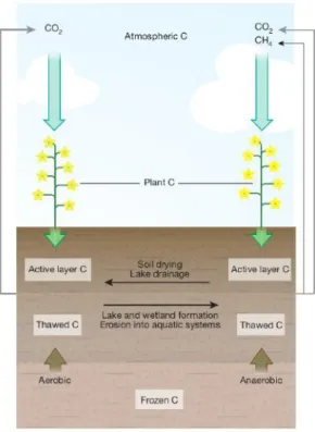
When these soil layers with sequestered C reach favourable conditions for mineralisation, such as warmer temperatures and access to oxygen, microbes ex- tract energy by breaking down the organic matter and release GHG into the atmosphere (mainly carbon dioxide (CO₂), methane (CH₄) and nitrous oxide (N₂O)) (Marushchak et al. 2011; Repo et al. 2009; Schaefer et al. 2011; Tamo- cai et al. 2009; Vardy et al. 2000). There, the GHG are radiatively active and store thermal radiation increasing global temperatures. A warming climate alters the C cycle and the permafrost areas turn from a C sink into a source for the atmosphere (Figure 1) causing a positive feedback to global warming - called permafrost carbon climate feedback (Strauss et al. 2017).

Figure 1: Permafrost Ccycle (Schuur et al. 2015). When the temperatures rise, the ALT increases and Cis released into the atmosphere.

For estimating C release, the soil composition as well as the hydrological regime are equally important. In anaerobic environments, C is released to a greater extent as CH₄, which has a 21 times higher potential impact on climate over a 100-years scale compared to CO₂ (IPCC 2013) whereas in aerobic environments the total loss of C is greater and has a higher impact on climate (Schuur et al. 2015). Depending on the amount of C in soil, the release of GHG differs significantly. Mineral (< 20% C) and organic (> 20% C) soils feature decade losses of 6-13% and 17-34% respectively (Schuur et al. 2015).

(16)

The magnitude of C release from permafrost soils is strongly linked to the C/N ratio (Table 1). Microbes breaking down C for energy, use nutrients such as nitrogen (N), which remain in the vegetation or the soil whereas C is released as GHG. Consequently, a wide C/N ratio indicates a low rate of mineralisation and hence the potential for further decomposing of C (Sollins et al. 1984;

Stevenson 1994; Strauss 2010; Walthert et al. 2004).

Under the current climate warming trajectory Representative Concentration Table 1: Classification of mineralisation rate according to C/N ratio in soils after Walthert et al. 2004

.

Pathway (RCP) 8.5, model scenarios suggest a potential C release from permafrost zones to be in the range of 37-174 Pg C with an average of 92 Pg C across models by 2100 (Schuur et al. 2015). This translates into a contributing warming potential of up to 0.27 °C by 2100.

As permafrost degrades, the thickness and areal extent decrease, the ALT deep- ens, taliks and lakes can develop and enlarge, and the landscape changes ge- omorphologically and GHG release is increased (Burn 2011; Everdingen 1998;

Kokelj and Jorgenson 2013; Kokelj et al. 2009; Romanovsky et al. 2017).

Strauss et al. (2017) mentions four different explanations why permafrost degrades: (I) An increased unfrozen water content and ground warming, (II) deepening of the ALT, (III) thermo-erosion along lakes, rivers and coasts and (IV) rapid thaw due to thermokarst and thermo-erosional processes. Morgen- stern (2012) points out that the two main reasons for permafrost degradation are thermokarsts and thermo-erosional processes which strongly modify the landscape and enhance permafrost degradation on a local scale. Understand- ing their dynamics regarding GHG release and landscape evolution is therefore highly important.

1.1.3 Thermokarst

Thermokarst terrain develops when ground ice melts or permafrost thaws and the soil collapses into the volume previously occupied by ice (Everdingen

(17)

1998). The process itself is termed thermokarst leading to typical thermokarst terrain and landforms. It enhances the permafrost degradation and microbial activity by lowering the water table and exposing previously cryotic ground (Kokelj and Jorgenson 2013; Romanovsky et al. 2017). Landforms with thermokarst features are mainly constrained to ice-rich glaciogenic deposits and are mostly absent from non-glaciated terrain and Holocene alluviums (Kokelj et al. 2017).

Preferentially, they evolve in environments with at least a slight slope gradient and excess of water and ice, causing large volumes of thawed material to be transported into fluvial, coastal and lacustrine environments (Chin et al. 2016;

Kokelj et al. 2005; Lantz et al. 2009; Shur and Jorgenson 2007).

Under varying conditions the thermal equilibrium can be disrupted by geomorphic, vegetational or climatic processes, either natural or man-induced.

Warmer air temperatures, increased rainfall and changes in snow and vegetation cover have been identified as main drivers of permafrost degradation (Biskaborn et al. 2019; Burn and Kokelj 2009; Kokelj and Jorgenson 2013;

Osterkamp 2007a,b; Romanovsky et al. 2010a,b; Shur and Jorgenson 2007;

Zhang and Stamnes 1998). These changes can cause a thermal disturbance of up to 6 °C compared to undisturbed ground (Burn 2011). Initiating events such as extreme thaw or high precipitation can result in thaw subsidence of permafrost causing the degradation of permafrost (Lacelle et al. 2010; Lantz et al. 2009).

Thermokarst development is generally expected to accelerate and intensify with warming temperatures, since more permafrost is affected by thawing (Kokelj and Jorgenson 2013; Murton 2009). Increasing thermokarst activity indicates a rejuvenation of post-glacial landscape by mobilising previously cryotic glaciogenic deposits transforming large parts of the landscape.

Thermokarsts and their impact are complex and consist of positive and nega- tive feedbacks. Several thermokarst landforms are associated with processes of permafrost degradation. One of the largest and most impacting thermokarst features on a local scale are retrogressive thaw slumps.

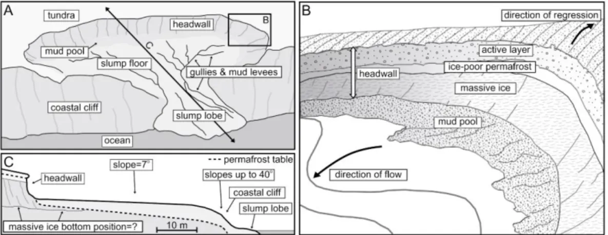
Retrogressive thaw slumps are big geomorphic features which can impact an area of tens of hectares and can displace volumes of a magnitude of 10⁶ m³of thawed material (Lantuit and Pollard 2008). Determining probable initiating events is problematic since large slumps take years to evolve and may exhibit a polycyclic nature referring to a development of new thaw slumps within the slump floor of older retrogressive failures (Kokelj and Jorgenson 2013). They occur along streams, rivers and coasts (mechanical erosion), at lakes (thermally driven) and at slopes (extreme thaw and precipitation events) comprising a distinct structure (Figure 2).

Ice-rich ground is exposed and ablated through retrogressive failure of the

(18)

soil at the headwall. Depending on the magnitude of the retrogressive failure, headwalls can be up to tens of metres high. Headwalls of thaw slumps at coasts can continue to retreat at rates of 10 metre per year (m/a) for decades and reach a peak headwall retreat of up to 30 metre (m) in exceptional years (Lantuit and Pollard 2005). At the slump floor debris accumulates and is transported downslope by rainfall-induced, fluvial and gravitational processes.

At the foot of a slump, where the slope flattens out, when no stream or river is erosively active, an alluvial fan-shaped lobe of debris can form.

Stabilisation of thaw slumps occur when sufficient material accumulates in

Figure 2: Schematic of retrogressive thaw slumps (A), headwall (B) and (C) cross-section structures after Lantuit and Pollard 2005

front of the headwall and vegetation starts to cover the slump area and impede further thawing of ground ice. It may be several decades before thaw slumps are stabilised (Burn 2011).

Generally, larger slumps retreat more rapidly due to positive feedbacks such as larger exposition to solar radiation, higher rate of ablation and more efficient debris transport. Kokelj et al. 2017 shows that the erosion intensity, the relative relief and therefore also the disturbance density is the highest at fluvial and coastal environments. Thaw slump activity has accelerated with climate change and is expected to increase in the future, in particular due to increases in rainfall (Gooseff et al. 2009; Kokelj et al. 2015b; Lantuit and Pollard 2008;

Lantz and Kokelj 2008).

Thermokarst development has gained scientific interest due to its implica- tion on the C cycle (Grosse et al. 2011; Turetsky et al. 2019). Roughly 20 % of the northern permafrost area is covered by thermokarst landforms and the unstable areas are also expected to be the most carbon-rich (Olefeldt et al.

2016). In recent literature the term “abrupt thawing” has evolved referring to fast developing thermokarst features which have a similar climate impact as gradual thawing thermokarst due to their greater release of methane (Koven et al. 2015; Turetsky et al. 2019). The presence of abrupt thawing is expected

(19)

to amplify C release by 50 % although effecting less than 20 % of the landscape (Turetsky et al. 2019).

To determine overall changes in permfrost regions, the analysis of specific soil parameters are necessary to reveal small processes within the soil effecting the landscape on a larger scale.

1.1.4 Soil Properties

In arctic regions, soil genesis is dominated by cryogenic processes due to its cold climatic conditions (Margesin 2009). Stresses and pressures created by expanding ice and contracting soil material due to temperature changes, translocate, rearrange and deform materials and solutes leading to unique soil characteristic in permafrost-affected soils. Dominantly, the presence and movement of unfrozen soil water towards the permafrost table drives these cryogenic processes such as freeze-thaw, frost heave, cryoturbation, thermal cracking, cryogenic sorting, cryodesiccation, gleying, eluviation, brunification and salin- ization (Bockheim 2007; Ping et al. 2008; Vandenberghe 2013). Although most of these processes occur in the AL, they also affect the near-surface permafrost due to fluctuations in permafrost table depth (Ping et al. 1998).

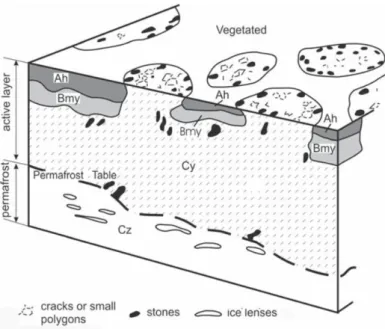
The subsurface soil horizons commonly exhibit a blocky, platy structure and are associated with higher bulk densities. Typical features are irregular and broken soil horizons, organic intrusions and accumulation, silt-enriched layers and caps, granular structures and vein formations disrupting the general horizontal organisations of the soil (Figure 3) (Ping et al. 2008; Tarnocai and Bockheim 2011; Tarnocai and Smith 1992; Vandenberghe 2013; Vardy et al.

2000). These characteristics define the movement of water through and the thermal properties of the soil dictating its past and prospective evolution.

When water percolates along the thermal gradient from warm to cold, it refreezes in the subsoil increasing the ice thickness and volume over time at the permafrost table. The occurrence of large ice volumes in permafrost has strong implications on the stability of soil (Chapter 1.1.3). This pattern is visible in moisture and soluble content profiles and fine organic and inorganic matter accumulation layers enriching the lower AL and near-surface permafrost in mineral and organic soils (Kokelj and Burn 2005; Kokelj et al. 2002; Tarnocai 1972; Wang et al. 2009). Relict active layer thicknesses can be determined by finding these accumulation layers (Kokelj et al. 2002).

In general, deeper layers have older organic material than upper layers due to the order of sedimentation and accumulation of organic C. Root penetration and soil reworking processes lead to mixed layers with differing ages. With aid of the 14C method, the age of each layer and the accumulation periods can be

(20)

Figure 3: Schematic showing a non-sorted soil profile with broken cryoturbated soil horizons (y), strongly indurated B-horizons (m), accumulated organic matter at surface (h) and accumulated solubles in the C-horizon (z)(Margesin 2009)

determined.

After the retreat of the glaciers, thermokarst activities and cryogenic processes reworked the soil and mixed the layers which may have led to younger OM in deeper layers (Akerman 2005; Lacelle et al. 2004; Pries et al. 2012). In particular, in the first metre of the soil the mixing of layers has been observed (Pries et al. 2012).

Cryoturbated soils in the arctic tundra of Canada contain substantially higher Soil Organic Carbon Content (SOCC) values compared to soils without cryoturbation (49 to 61 kilograms per square metre (kg/m²) compared to 12 to 17 kg/m²respectively) (Tarnocai and Bockheim 2011). According to King et al.

(2008) organic soils consist of much higher organic content (43 to 144 kg/m²) than mineral soils (49 to 61 kg/m²). The rates of organic Caccumulation are controlled by different environmental factors such as orientation, slope angle or nutrition availability (Chapin et al. 2002; Pries et al. 2012; Shaver et al.

1992).

In contrast to these vast organic accumulations in the AL and the permafrost, N contents are generally very low (<1 gravimetric percentage (wt%) or<10 g/kg TN) limiting plant growth and are mainly stored in the surface organic matter and the vegetation and decline with increasing depth (Broll et al. 1999).

N can only be taken up by living plants where roots can penetrate the soil and the uptake of N is therefore restricted to the AL. Other processes of N deple- tion is through microbial activity releasing the GHG N₂O into the atmosphere (Chapter 1.1.2).

(21)

The C/N ratio is narrow in the AL indicating the rate of mineralisation (see Chapter 1.1.2, Sollins et al. 1984; Stevenson 1994; Strauss 2010; Walthert et al. 2004). It is wider in the permafrost where perennially cryotic ground pro- hibits mineralisation and similarly wide in the lower layers of the AL due to anaerobic conditions (Weintraub and Schimel 2005) releasing GHG at a much slower rate (Gundelwein et al. 2007; Hinkel et al. 2001; Lacelle et al. 2010;

Schuur et al. 2015; Tarnocai and Bockheim 2011; Vardy et al. 2000; Wang et al. 2009). High organic material leads to lower bulk densities which increase with depth when the OM diminish and the soil texture changes to having more consolidated material (Vardy et al. 2000).

Studies mention dynamics where sediments are mobilised leading to a deple- tion of finer sediments in upper layers, a process occurring since the Holocene warming period to varying extents (Lacelle et al. 2004; Locke 1986). As silt is more prone to translocation developing silt-enriched layers and silt caps in the AL and as water mobilises finer sediments (clay and silt), a grain size differentiation can be observed (Bockheim and Tarnocai 1998; Lacelle et al. 2004;

Locke 1986; Tarnocai and Bockheim 2011).

This study examine the changes in soil parameters between disturbed and undisturbed ground mainly at retrogressive thaw slumps. Disturbance categories are therefore introduced for comparison.

1.2 Site description

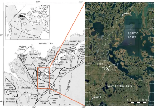
The study area is located north of Inuvik, Northwest Territories, Canada, south-east of the Mackenzie River Delta (Figure 4). It lies in the Mackenzie region where elevations vary between 9 and 187 m above sea level. The terrain with gently rolling hills and some deep river valleys has a mean slope angle of 3 °(Marsh et al. 2010).

The underlying bedrock is primarily Cretaceous and Tertiary clastic and sed- imentary rock (Dixon et al. 1992; Rampton 1988). The arctic coastal plain north of Inuvik is characterised by Pleistocene coarse grained fluvial, deltaic and estuarine sediments overlain by extensive sheets of ice-containing sediments with interbedded peat layers covered with morainal deposits and a thin organic layer on top (Mackay 1963). According to Rampton 1988 the study area is subdivided into the Anderson Plain with the South Caribou Hills and the Tuktoyaktuk Coastal Plain with the Eskimo Lakes Pitted Plain (Figure 4).

All sampling locations apart from Lake 6 lie within the elevated Caribou Hills (Rampton 1988). Sample site Lake 1 lies in the centre of the plain whereas Lake 11, 12, Trail Valley Creek (TVC) and 1sub3 at the boarder to the Eskimo

(22)

Figure 4: Physiographic subdivision of Tuktoyaktuk Coastlands and adjacent areas of the Geological Survey Canada (Rampton 1988) (left). The study area lies within the South Caribou Hills and the Eskimo Lakes Pitted Plain. Eskimo Lakes are north of most study sites apart from Lake 6 which lies west of them.

Overview map of study sites (right). White line indicates the Tuktoyaktuk- Inuvik-Highway. Dashed line indicates the north-eastern boundaries of the South Caribou Hills modified from Rampton 1988. Background map is created with an satellite imagery map from 2017 provided by Google (Google Maps 2017).

Lakes Pitted Plain. The site Lake 6 is located at the Eskimo Lakes further north. More detailed maps are displayed in the appendix from Figure A2 to A11.

The Caribou Hills is a bedrock controlled landform and is well elevated above the surrounding area. The surficial geology of the study area is dominated by morainal deposits developed during the Toker Point Stade of the Early Wisconsinan glaciation (Pleistocene). It consist also of galciofluvial out- washs from plain and valley trains around the Eskimo Lake (Late Wisconsinan glaciation, Sitidgi Stade), lacustrine deposits around relict or still existing lakes (< 15% lake cover (Mackay 1963)) and colluvial deposits formed later in the Holocene (Rampton 1987).

At the outer perimeter, the area is characterised by sharp escarpments in the east and north but more gentle in the south leading to a radial drainage system with broad melt-water channels. Except from small depressions, the Caribou Hills are well drained with thin unconsolidated, coarse-grained material which often is more than 13 m thick (Rampton 1988). There are well-laminated and

(23)

cross-bedded silts, sands and gravels inter-stratified with up to 90 centimetres (cm) thick peat beds. They indicate a previous position of the Mackenzie Delta due to post-glacial changes in sea level and a possible different course of the Mackenzie River into the Liverpool Bay (north-east of study site in Figure 4) with climatic conditions probably similar to the present (Mackay 1963). The landscape at the Caribou Hills was highly modified by thaw processes in the past which abated and permafrost could accumulate again (Kokelj et al. 2002).

According to Dyke and Prest 1987 large parts of the Mackenzie Delta and its margins were deglaciated ca. 12-13 10³ years (ka) ago but organic material did not begin to accumulate before 8 ka ago - at least in this study area (Clark et al. 2009; Dyke and Evans 2014; Kitover et al. 2016).

The current climate is characterised by long cold winters and short sum- mers, with a snow cover period of 8 months. The mean annual temperature is -10°C and the mean annual precipitation is roughly 260 mm whereof 60 % falls as snow (Marsh et al. 2010). Rampton 1988 determined an annual near-surface ground temperature between -5 and -6°C in the Caribou Hills but recent data mentioned temperatures up to -1.7°C (Gr¨unberg et al. 2020). The study area is underlain by ice-rich continuous permafrost at the edge of the forest-tundra transition zone. Extensive sheets of ice are common with an AL ranging from 0.3 to 0.8 m at sites without apparent permafrost degradation (Marsh et al.

2010).

Compared to other regions in Northwest Territories (e.g. The Peel Plateau), the study area features a low density of thaw slumps due to gentle topographic gradients and abated thawing after the early Holocene warming period (Mur- ton 2001). It is known to have experienced strong modification by thermokarst processes in the past shaping todays landscape (Rampton 1988).

1.3 Disturbance categories

Disturbance categories are implemented to connect permafrost degradation with certain soil processes. Based on experience and visual classification of the sites, disturbed-categorised ground (in plots and table referred to as ”yes”) is expected to develop a distinct pattern compared to non-disturbed ground (”no”).

Each sample location was categorised according to its aforementioned level of degradation. For assigning each sample location to its category, maps, the field book notes and pictures are advised. Aerial pictures and satellite images are commonly utilised for visual classification and identification (Kokelj et al.

2015a,b; Lacelle et al. 2015; Lantz and Kokelj 2008).

(24)

Inside the head wall the ground is categorised as disturbed, often indicated by bare soil at the surface (sign of soil erosion) with no vegetation on top (Figure 5a). Samples taken at the headwall and the close proximity of it, are also categorised as disturbed since it is the position of ablation where thaw slumps advance and enlarge (Figure 5b).

The vegetation cover is also taken into account when categorising the sites (Burn 2011; Burn and Friele 1989). High and dense vegetation has proven to be an indicator for disturbance but is no prerequisite for disturbed ground (Figure 6). At water bodies and small channels with apparent flowing or standing water a disturbance is also expected due to the thermal influence of the water (see Chapter 1.1.3) (Kokelj and Jorgenson 2013).

Areas not effected by disturbances are identified by no obvious presence of soil erosion or mass movement indicated by the typical short vegetation cover (Figure 7). The absence of standing or flowing water is also important when categorising sites as undisturbed.

(a) Bare soil inside the thaw slump at Lake 6 indicates typical slope failure and mass movements. In the far back of the picture the headwall stands out. (Picture taken from inside the thaw slump at Lake 6 on 20th of August, 2018 by Julia Boike, Alfred- Wegener Institut, Helmholtz-Zentrum f¨ur Polar- und Meeresforschung (AWI))

(b) A strongly exposed, vertical headwall section at Lake 6 (Picture take on 20th of August, 2018 by Bill Cable, AWI).

Figure 5: Examples of sites categorised as disturbed at Lake 6 [69.0066 North- ern decimal latitudinal degrees (North), 133.3634 Western decimal longitudinal degrees (West)].

(25)

(a) Picture taken from headwall downwards towards the lake. Thaw slump is in the centre of the picture.

(b) Picture taken upwards towards the head wall from inside of the thaw slump visible in Figure (a).

Figure 6: High vegetation with willow shrubs (a) and high grass cover (b) in and around the thaw slump are typical for highly disturbed areas. Location at Lake 6 [69.0066 North,133.3634West] (Pictures taken on 20th of August, 2018 by Inge Gr¨unberg, AWI).

Figure 7: Typical site defined as undisturbed without any sign of soil erosion or depressions. Typical vegetation cover are lichens, tussock sedges, tundra moss and dwarf shrubs [69.0066 North,-133.3634 West] (Pictures taken by Inge Gr¨unberg, AWI).

2 Methods

2.1 Sample extraction in-situ

The data was obtained during the MOSES expedition¹ to the Northwest Territory of Canada in August 2018. Permafrost and/or AL samples were taken at six different locations along the Inuvik-Tuktoyaktuk-Highway. The locations Lake 1, TVC and 1sub3 were sampled at undisturbed sites (Figure A2 and A5). At Lake 6, 11 and 12 several sample points were set along a

1https://www.ufz.de/export/data/470/236390_mCAN2018_Report.pdf(Accessed on 25th June 2020)

(26)

transect from undisturbed tundra through retrogressive thaw slumps to lake shores (Figure A3, A4 and A6). At Lake 1, TVC and 1sub3 a pit was dug through the AL down to the frost table boundary for permafrost core extraction (Figure 8). The battery powered mini-SIPRE Coring Auger (Figure 9) drills

Figure 8: Lake 1, first pit after drilling the first core. (Picture take on 17th August, 2018 by Julia Boike, AWI)

down to almost one metre with a coring barrel extracting a core of 5 cm in diameter. Depending on the composition of the ground (e. g. stones inhibit the drilling), the auger extracted cores of 7-60 cm in length.

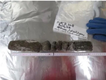
The parts were subsequently packed in plastic bags (Figure 10). During this step, care had to be taken to label the depths of each core section accurately and indicate the top and the bottom of the core.

Frozen samples were put within hours of sampling into a freezer and all samples were transported in a cooling container with ice packs back to Ger- many. The ice packs were successful in keeping the samples frozen during the journey, as shown by the temperature data collected by a logger in the cooler.

The AL soil samples were taken at different depths in the same pits where frozen core samples were drilled. The samples were simply filled into Falcon tubes or into plastic bags. Additionally, at each site the ALT and the vegetation types were noted.

At sites where no pit was dug, AL soil samples were extracted with a 2 cm in diameter soil sampling probe² extracting samples from a maximum depth of 1 m.

The extended data set with ALT measurements of Inge Gr¨unberg, AWI exhibits a different sampling setup than the main data set. Although the areas remain the same (e.g. Lake 1, 6...etc.), there are more sampling positions in each area than obtained for the main data set. Detailed maps are shown in

2https://www.ams-samplers.com/7-8-x-33-sst-soil-probe-w-handle.html [Ac- cessed on 26th June, 2020]

(27)

(a) (b)

Figure 9: (a) Testing of the battery powered mini-SIPRE Coring Auger at Lake 1 - Position 1 [68.575479 North, 133.73358West] (Picture taken on 17th of August, 2018 by Julia Boike, AWI); (b) One metre coring barrel extracting a 5 cm in diameter core (Picture taken by Frieder Tautz)

the appendix (Figure A7 to A11).

2.2 Acitve layer and permafrost subsampling

The cores were taken out of the freezing room (-25°C) and aligned along the folding rule on aluminium foil in the cooling chamber (-4°C) giving an overview over each core (Figure 12). Not every subsection (individual pieces of the core) was sampled for every parameter. It was decided for each core section individually what subsamples are to be taken. Leftovers, referred to as

“Extra” were saved for further or repeated analyses (Figure 13).

Ideally, the subsamples were extracted from the centre of the core since the outside of the core was not representative caused by thawing and refreezing during transportation. Evidently thawed parts or pieces of the core which could not be assigned properly to the core sequence, were cut off and discarded.

The weight of the sub-samples was acquired, together with the Nasco Whirl-Packs plastic bags, so that the actual weight of the sample could be calculated by subtracting the average weight of one bag. The tools for dissect- ing the subsections were a knife and Makita band-saw.

Firstly, each core was sampled at least once for 14C. A few grams were put

(28)

(a) (b)

Figure 10: Aligning the core after drilling (a) and packing it in plastic bags (b) at Lake 6, Pit [69.033713 North, 133.253694West] (Picture taken on 20th of August, 2018 by Julia Boike, AWI)

Figure 11: AL soil samples taken at study site Lake 11 on 24th August, 2018 (Pictures on 6th and 7th November, 2018 taken by Frieder Tautz)

into an annealed jar with aluminium foil underneath the lid. These samples were analysed in the AWI laboritories MICADAS in Bremerhaven.

Secondly, suitably sized subsections were cut with the band-saw into cuboids or cylinders and determined for their volume and their weight. These samples were used to analyse the ice content and the according bulk densities in the AWI laboratories in Potsdam.

Thirdly, small pieces were put into plastic cans for the analysis of TOC, TC, TN and grain size in the AWI laboratories in Potsdam.

Further subsamples were taken from soil samples extracted from above the frost table boundary. They have been kept frozen after being taken from the soil and subsampled for TOC, TC, TN, grain size and 14C. The 14C subsamples were only taken once per soil profile.

(29)

Figure 12: First core taken at Lake 1 at the first pit aligned on aluminium foil in cooling chamber at -4°C (Picture taken on 15th of November, 2018 by Frieder Tautz)

2.3 Laboratory Analyses

The following analyses were conducted for this thesis’ objectives. All measurements done in the laboratories at AWI, Potsdam were obtained by the author.

The other measurements were send to the appropriate laboratories of AWI.

• Biochemistry: TC, TN, TOC (AWI Potsdam)

• Grain size analysis (AWI Potsdam)

• Ice content (AWI Potsdam)

• Radiocarbon dating (¹⁴C) (AWI, Bremerhaven)

2.3.1 Biochemistry

The quantitative analysis of TC, TN and TOC of the samples were determined with the gas-phase chromatograph (Elementar Analysensystem GmbH Vario MAX-C for TOC; Elementar Analysensystem GmbH Vario EL III for TC and TN). The main principle of gas-phase chromatography is based on catalytic tube combustion with oxygen supply at high temperatures to incin- erate the compounds of the sample and change the aggregate state to gaseous.

With an unreactive carrier gas (mobile phase), the gaseous sample is then transported through a tube/column with a specific filling (stationary phase) interacting with the gas. Each compound takes different times to pass through and exit the column due to different chemical and physical properties (retention time). Since the compounds are separated from each other and the elements are detected and identified electronically, it is possible to analyse each element qualitatively and quantitatively.

(30)

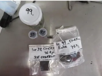
Figure 13: Subsampling for different analyses in cooling chamber: Nasco Whirl-Pack referred to as “Extra” as backup samples for subsequent analyses if necessary and the cuboid for ice content. The plastic tins are for TOC, TN, TC and GSD. The 1.5 millilitre (ml) Safe-Lock Tube for microbial sequencing (data not included in this thesis). The glass jar for 14C analysis. (Picture taken on 6th of November, 2018 by Frieder Tautz)

The subsamples for the biochemical analysis (TOC, TC, TN) were freeze- dried (Sublimator 2-4-5, Zirbus Technology) and subsequently milled in agate grinding jars (Planetary mill Pulverisette 5, Fritsch). Of the ground material 8

±0.005 milligram (mg) was filled into 50 mg tin boats together with tungsten oxide for assuring complete incineration of the sample. These small containers needed to be folded in such a way that no material is being lost during the process, because the exact weight of the sample is crucial for the analysis. The TOC samples were put and weight into crucibles instead of tin boats. The amount was dependent on the TC values obtained beforehand.

Additionally, the gas-phase chromatograph required standard samples every 15 measurements with known amounts of the measured compounds to ensure correct analytical values, which were also filled into the tin boats or crucibles respectively. To eliminate possible errors each sample is measured twice.

2.3.2 Grain size analysis

This analysis is based on the diffraction of light by particles passing through a laser beam. The intensity of the light scattered by a particle is directly proportional to the particle size and indirectly proportional to the angle of the laser beam (Fraunhofer diffraction).

The organic compounds of the sample needed to be removed with Hydro- gen peroxide (H₂O₂) to measure only clastic grains. For at least two weeks, 10 ml of 30% acetic acid (CH₃COOH) was added daily to the dried sample mixed with a 3 % H₂O₂ solution.

(31)

The pH had to be controlled by adding Ammoniac or CH₃COOH accordingly to ensure the pH to be within the range of 6.5-8. The samples were put on a heating shaker at 60°C to enhance the reaction and inhibit conglomeration at the bottom of the beaker glasses (Edmund B¨uhler GmbH SM 30 AT con- trol). When the reaction of the acid with the sample attenuated significantly (reaction indicated by bubbling) and there was no further significant change in pH observable, it was centrifuged to suck up most of the H₂O₂ and water (Heraeus Cryofuge 8500i, Thermo Scientific) and freeze-dried afterwards (Sublimator 2-4-5, Zirbus Technology).

Less than 1 gram (g) of the sample (depending on the texture of the sample) was then weighed and filled into plastic bottles with a spoon sodium pyrophosphate and a one per cent diluted ammonia solution. The sodium pyrophosphate creates a mantle around each grain to impede agglutination of single grains. To ensure that all grains were separated from each other, the plastic bottles were put in a rotation shaker for at least one day (RS12 Rotoshake, Gerhardt).

Concerning the limitation of the grain size analysis, the measurements were restricted to grains smaller 1 millimetre (mm) removed mechanically with a 1-mm-sieve. The weight of the sieved grain fractions smaller and larger than 1 mm are obtained to determine how much of the grain fraction is not included in the grain size analysis (A1). This methodical error needs to be addressed accordingly and is indicated by the fractions larger than 1 mm in [wt%] removed with the sieve and the relative amount of grains (>1mm) measured by the Mastersizer3000 (see Chapter 4.5).

To ensure a grain density obscuring the light between 2 and 15 %, a conic rotary sample divider (Laborette 27, Fritsch) divided the solution into 8 equally grain-distributed sub-samples. A sieve on top of the conic rotary sample divider filtered grains larger than 1 mm which were dried and weighed afterwards.

The samples smaller than 1 mm were afterwards analysed with the grain size analyser (Malvern Mastersizer 3000 Hydro-LV).

The analysing device measured the light, obscured by the water in the tank beforehand, to calibrate the measurement of the grain size. The water level needed to be manually adjusted so that the grain density was within the obscuration range. At least three of the eight subsamples (from the rotary sampler) needed to be analysed. For each sample the device measured the GSD at least three times to ensure a statistical representation of the probe.

The programme of the Malvern Mastersizer 3000 calculated averages, variances and deviation for each sample.

(32)

2.3.3 Ice content

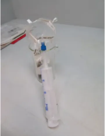
After the thawing of the cylindrical or cubic samples, the water was extracted from the sample with a 5cm-Rhizon soil moisture sampler and a vacuum tube for further chemical analysis not included in this thesis (Figure 14).

Out of 16 samples only seven were suitable for water extraction. The oth- ers did not contain sufficient water content for extraction. By applying the vacuum, water was sucked through the membrane of the Rhizon soil moisture sampler into the vacuum tube. In order to ensure that no air was drawn in and the Rhizon was fully submerged in the sample, the plastic bags were pressed together with tape. The samples after the extraction were freeze-dried to de-

Figure 14: Setup of Rhizon soil moisture sampling in the AWI laboritories in Potsdam (Picture taken by Frieder Tautz)

termine the total water content which was calculated from the difference in weight before and after the extraction and freeze-drying. Wet (ρ_w) and dry (ρ_d) bulk densities in [g∗cm^–3] were calculated using the respective wet (m_w in g) and dried (m_d in g) weight and the volume (V) of the samples (Equa- tion 1). The volume was obtained during subsampling in the cooling chamber by cutting cubes or cylinders out of the core and measuring these for their volumetric dimensions.

ρ= m

V (1)

The volume of ice/water (V_i in cm³) in a sample was calculated with the difference in weight before (m_w in g) and after (m_d in g) removal of the water and an assumed ice density (ρ_i in g∗cm^–3) of 0.9167 g∗cm^–3 (Glen 1958) (Equation 2).

V_i = mw– m_d

ρ_i (2)

The ice content can also be calculated as volumetric (θ) with Equation 3 and gravimetric (u) ice content with Equation 4 where V_g is the total volume of

(33)

the probe.

θ = V_i

V_g ∗100 (3)

u = mw– m_d

m_d ∗100 (4)

2.3.4 Soil Organic Carbon Content

With TOC values [wt%], the contribution of each layer (SOCC_Layer) to the total SOCC of the profile can be retrieved with Equation 5 derived from Strauss 2014; Tamocai et al. 2009. The SOCC is the overall TOC [kilograms (kg)] per area unit [square metres (m²)]. To obtain the SOCC at each site, the SOCC of all layers at the site are summed up. This calculation enables comparison between sites just for soil profiles with an equal amount of measurements or of soil profiles where sampling has been conducted for each soil horizon (1sub3 and Lake 11 - Position 4). T is the layer thickness in [m].

SOCC_Layer = TOC

100 ∗ρ_d∗1000∗T (5)

To enable comparison between all sites, each SOCC value per layer is reduced to the amount of SOCC per unit layer depth and is then averaged over all values of each profile (n is the number of observations). Multiplying it with the reference depth of 1 m calculates the averaged amount of SOCC per cubic metre soil [kg/cubic metres (m³)] (Equation 6).

SOCC_profile =

P(SOCC_Layer/T)

n ∗100 (6)

Since the dry bulk density (ρ_d) is not acquired for every layer, it is average over the whole data set.

2.3.5 Radiocarbon dating

The age determination was conducted in the AWI laboratories in Bremer- haven, MICADAS³ with the radiocarbon dating method (14C) on organic plant material making use of the radioactive decay of the carbon-14 isotope (¹⁴C) nuclide. There are three existing isotopes of C: carbon-12 isotope (¹²C), carbon-13 isotope (¹³C) and the most stable ¹⁴C. The ¹⁴C isotope originates from the reaction of stable nitrogen-14 isotope (¹⁴N) with solar neutrons in the upper troposphere and in the stratosphere and exhibit a certain propor-

3https://www.awi.de/en/science/geosciences/marine-geochemistry/micadas.html [9.10.2020]

(34)

tion in the atmosphere (approximately one¹⁴C atom per 1012 stable C atoms).

Hence, they are part of the C cycle. Living organisms absorb and metabolise the C atoms through photosynthesis assimilating CO₂. After the organisms death the ¹⁴C nuclide decays into the more stable N at a constant rate and the ratio between ¹⁴C and ¹²C diminishes consequently. The radioactive half- life of ¹⁴C, the time after which half of the ¹⁴C atoms are decayed, amounts 5730±40 years (a) (Dawson and Brooks 2001; Godwin 1962). The correspond- ing time since the organisms death (t in a) can be calculated with equation 7 where the decay constant λ is in [a^–1], the original ¹⁴C content (¹⁴C_t=0) and the ¹⁴C content after a certain time (¹⁴C_t=1) in [percent modern C] (Libby 1961; Stuiver and Polach 1977). The unit [percent modern C] is the¹⁴C value from 1950 for the purpose of comparison of papers throughout history.

t = 1

λ ∗ln

14C_t=0

14C_t=1 (7)

The method with the Accelerator Mass Spectrometer (AMS) determining the isotope ratios, has a detection limit of approximately 50.000 a (Fairbanks et al.

2005).

2.4 Statistical approach

All of the statistical analyses and visualisations are conducted with the programme R - Version 3.6.3 and LibreOffice Calc. Maps are created with QGIS OpenSource - Version 3.10.4 - A Coru˜na.

At two sites the ALT was not obtained due to the limits of the active layer probe (100 cm) used to assess the ALT, noted with a ”larger than” sign. For the statistical analysis the value is set to the highest possible value, hence 100 cm.

The biochemical data was handled similarly. The devices accuracy is limited to its lowest value of 0.1 wt%. Any values below that are displayed accordingly (< 0.1 wt%), yet it is set to exactly 0.1 wt% to include the values in the statistical analysis. The gravimetric percentage is transferred into a more useful unit of [g/kg] by multiplying the value [wt%] by 10. The difference between categories is determined by their mean.

The ALT has been acquired at more positions than otherwise included in the data set. The comparison of the ALT among sites includes additional ALT measurements acquired during the same expedition by Inge Gr¨unberg, AWI.

It is only used for plots concerning the ALT to ensure a higher number of values and hence a higher significance when making deductions. This data set includes ALT measurements at sites far away from any thaw slumps and the

(35)

definition of disturbance is not just restricted to thaw slump activity but it contains sites far away from any lakes and/or thaw slump activity (Chapter 1.3). When referring to other parameters than ALT, the data set is reduced to the number of samples analysed in the laboratories.

The 14C data analysed in the AWI laboratories in Bremerhaven needed to be calibrated according to the historical ¹⁴C/¹²C ratio. The raw data from the laboratories are calculated with a constant historical ratio between those two isotopes in the atmosphere and hence a constant exchange between the vegetation and other reservoirs is falsely assumed. Different ¹⁴C archives have shown that the ratio has been highly variable over the course of time (Fairbanks et al. 2005; Libby 1961; Reimer et al. 2013; Stuiver and Polach 1977). This is why the radiocarbon age has been calibrated with the INTCAL13 data set from 2017 (Reimer et al. 2013).

Outliers in the boxplots were checked for potential sources of sampling errors in the data. Any disruption in the general horizontal layer structure, observed as outliers in the data, are removed from the statistical analysis.

They indicate a vertical transportation of material and a clear processes of cryoturbation. To analyse any other processes apart from cryoturbation, vertical transportation of material needed to be identified and excluded since a cryoturbated ground features different values than a layered soil profile. The layers at Lake 6 - Position 1 (30-35 cm layer depth) and 1sub3 (70-80 cm layer depth), exhibiting cryoturbating characteristics visible in the pictures taken at the sites, are therefore excluded (Figures 15a and 15b). Any other outliers with no apparent reason for removal from the statistical analysis, remain in the data set. Outliers particularly discussed for exclusion are at Lake 11 - Position 4 (10-20 and 40-46 cm layer depth) and Position 6 (50-70 cm layer depth) but owing to lack of pictures or any other reason for removal, these values are to remain in the data set.

Measurements from AL and permafrost layers are compared to determine any differences between the permanently cryotic and the non-cryotic parts of the soil. Whenever the layer depth of a measurement (biochemistry, grain size) is relevant, the middle depth between the layer boundaries is determined.

To find any pattern in the GSD, the layers with grain size measurements from the AL are categorised according to their layer depth. There are three categories introduced: 0-30 cm, 30-70 cm and 70-100 cm.

Tests of significance are performed with the Welch’s two sample T-Test (α= 0.05). Correlation is calculated with Pearsons correlation coefficient r.

(36)

(a) The horizontal layer structure is disrupted due to cryoturbating processes [69.033713 North, 133.253683West]

(Picture taken on 20th of August, 2018 by Julia Boike, AWI) Site: Lake 6 - Position 1.

(b) Although a horizontal structure can be determined, in particular in the lower part of the AL profile, irregularities are a sign of cryogenic processes [68.740759 North, 133.494441West] (Picture taken on 26th of August, 2018 by Julia Boike, AWI). Site: 1sub3

Figure 15: Soil profiles with visible cryotic processes indicated by the white line and arrow. Outliers occuring at the depths of these discontinuities are excluded from further statistical analysis.

3 Results

3.1 General properties

The 69 measurements are distributed over 13 different positions east of the Mackenzie Delta at 6 different sites. There are 34 AL and 35 permafrost measurements from a maximum depth of 1.22 m.

The gravimetric and volumetric ice content amounts on average 60.6 wt%

and 73.0 volumetric percentage (vol%) respectively for the 16 samples obtained for ice content acquisition. The ice content in this study remains within the range of 36-81 wt% and 59-85 vol%. Most ice-content data were acquired at Lake 1, an undisturbed site in the proximity of a lake, featuring the highest values in the data set (Figure A2). The other four ice content measurements at 1sub3, TVC and Lake 6 - Position 2 are lower.

Soil profiles with no evident sign of permafrost disturbance (TVC and 1sub3) exhibit quite low ice content values similar to the only ice content measurement at a disturbed site (Lake 6 - Position 2). In general, the volumetric ice content decreases with increasing layer depth below the frost table (r = -0.64).

The wet and dry bulk densities of the samples taken from the permafrost are on average 1.2 and 0.5 g ∗cm^–3 respectively. Such as the ice content measurements, bulk densities were only obtained for permafrost cores but also