Research Collection
Working Paper
Modeling crossroads in MATSim
The case of traffic-signaled intersections
Author(s):
Sallard, Aurore; Balać, Miloš Publication Date:
2020-08
Permanent Link:
https://doi.org/10.3929/ethz-b-000429954
Rights / License:
In Copyright - Non-Commercial Use Permitted
This page was generated automatically upon download from the ETH Zurich Research Collection. For more information please consult the Terms of use.
ETH Library
2
Aurore Sallard 3
IVT 4
ETH Zurich 5
CH-8093 Zurich 6
aurore.sallard@ivt.baug.ethz.ch 7
8
Miloš Bala´c 9
IVT 10
ETH Zurich 11
CH-8093 Zurich 12
milos.balac@ivt.baug.ethz.ch 13
14 15
Word Count: 7459 words+0 table(s)×250=7459 words 16
17
Submission Date: August 1, 2020 18
ABSTRACT 1
In transportation simulation, the prediction accuracy of travel times on road segments can have sub- 2
stantial impacts on the simulation outcomes. The travel times are impacted, among other things, by 3
traffic signals. Modeling traffic signals is not straightforward in large scale simulations, especially 4
when data on their characteristics is not available. Due to this, in most of the applications using 5
the agent-based transport simulation software MATSim, traffic signals are not explicitly modeled.
6
This paper addresses this issue and proposes a method based on Webster’s formula to compute de- 7
lays experienced by motorists at traffic-signaled intersections without having access to the actual 8
traffic signal data.
9
Within this study, results regarding the imputation of road flow capacities and estimating 10
the impacts of congestion and crossroads on travel times will be presented and investigated. Ev- 11
idence shows that Webster’s approach and road capacity modifications can substantially improve 12
the quality of the travel time estimates for the regional model of Zurich, Switzerland.
13 14
Keywords: Traffic lights, crossroads, MATSim, Webster’s formula 15
INTRODUCTION 1
The goal of transportation simulation is to computationally reproduce travel conditions 2
within a given area, in order to assess the effects of future policies, investments, and, more gener- 3
ally, changes in the infrastructure. For this purpose, it is of primary importance to calculate travel 4
times as accurately as possible, because those strongly impact essential simulations’ results, such 5
as transport mode choice or destination choice. Travel times obviously depend on the length of 6
the chosen routes and of the speed limits enforced in the network. They are also influenced by 7
other parameters, such as congestion level, road geometry or zebra crossings. Road intersections, 8
as well, cause additional delays to motorists. This is why a special attention has to be paid to the 9
modelling of crossroads before actually running the simulation.
10
This issue is only partially covered in the default settings of the agent-based transport 11
simulation software MATSim (Horni et al. (1)). By default, no distinction is made in MATSim 12
between the traffic-signaled intersections and the other ones. Additional modules presented in 13
Grether (2) and Thunig et al. (3) offer however the possibility of adding traffic lights to the network 14
and to implement different strategies for controlling the signal schedules. They rely on a detailed 15
description of the intersections and on signal plans that had to be manually collected. Thus, those 16
approaches could be counted as work within the field of microscopic scale simulation, whereas 17
MATSim is usually used for mesoscopic scale applications.
18
This paper presents a contribution towards another possible way of modeling traffic- 19
signaled intersections within the MATSim framework, which relies on the Webster formula (Web- 20
ster (4)). This equation computes the optimal (in the sense of minimizing the average delay per 21
motorist) traffic signal cycle length. The presented approach does not model each individual signal 22
phase, but uses the average experienced delay, obtained through the Webster formula, to get more 23
accurate estimates of the travel times. This study also provides a straightforward way of adding 24
traffic lights’ localizations into an existing MATSim network and compares empirical travel times, 25
computed according to this new approach, to estimates obtained from two web APIs.
26
After presenting with more details the best-known methods for traffic signal scheduling 27
and the work already done within this field in MATSim, the present paper will guide the reader 28
through the different implementation steps of this new approach and provide insights into valida- 29
tion results.
30
BACKGROUND 31
Webster’s approach for optimizing the cycle length of traffic signals 32
One of the first approaches aiming to optimize the traffic signals’ schedule was described 33
by Webster. The chosen minimization criterion is the average vehicle delay, and, in this work, the 34
author develops a formulation for the optimal cycle length derived from equations approximating 35
the expected vehicle delay.
36
The computation of this average delay was thoroughly studied in Rouphail et al. (5). A first exact equation was proposed in Beckman et al. (6); it is valid for fixed-time signals under the
assumption of a binomial arrival process. Knowing the signal cycle lengthC, the effective green- phase length on a given linkg, the arrival rateqon this link, the departure rate Sfrom the queue during the green phase and Qo the expected overflow queue remaining after previous cycles, the expected delayd is given by
d= C g C
1−q
S
Qo
q +1+C g 2
. (1)
Furthermore, efforts have been made to approximate the expected vehicle delay by com- bining theoretical analysis and numerical simulations in contexts where this exact equation cannot be used, which can be due to several reasons. First, it is difficult to access the exact arrival and departure rates. Secondly, computing the expected overflow queueQocan also be a complex prob- lem. Finally, the assumptions underlying the exact formulae do not necessarily cover a large range of real-world situations. The first approximate formula was developed in Webster (4). According to this work, the average delay per vehicled, given in seconds, can be approximated by
d' C
1−g
C 2
2 1− g
Cx+ x2
2q(1−x)−0.65
C
q2
1 3x2+5
g
C, (2)
where 1
• Cis the cycle length in seconds;
2
• gis the effective green time reserved to the link on which the vehicle approaches;
3
• xis the degree of saturation on this link, which means the ratio of the (hourly) flow on the 4
link to the link capacity;
5
• qis the vehicle arrival rate in vehicles per second.
6
It has to be remarked that, if the first two terms of this expression have a theoretical justification, the 7
last one was designed only so that the theoretical delays fit better with values obtained empirically.
8
Given this expression, Webster derives from it a formula for the optimal cycle length Coptin seconds:
Copt:=1.5×L+5
1−Y , (3)
where 9
• Lis the total lost or unusable time during a signal cycle, in seconds. It corresponds to the 10
sum of the time lost due to clearance times after each phase and of the time when all the 11
traffic lights are red;
12
• Y is the sum of the saturation ratiosxfrom 2.
13
The effective green time,G:=Copt−L, can finally be split among the incoming links according to 14
their contribution to the total flow.
15
Webster’s formula has been successfully used in transportation analysis for decades and 16
remains one of the prevailing approaches to optimize traffic signal operations. It has been adapted 17
in several recent works. For instance, in Cheng et al. (7), the same optimization criterion was con- 18
sidered, but another approximate equation for the expected delay was used. Furthermore, with the 19
recent rise in interest for more environmentally sustainable transportation systems, this approach 20
was adapted in Calle-Laguna et al. (8) and Calle-Laguna et al. (9), considering new measures of 1
traffic signals’ effectiveness, namely fuel consumption and emissions of pollutants.
2
Lämmer’s adaptive traffic signal control algorithm 3
Numerous other ways of scheduling traffic signal operations have been proposed. Some 4
of them, such as Babicheva (10), rely on recent findings of queuing theory, others, such as Tonguz 5
et al. (11), are based on cellular automata approaches. It would be impossible to review throroughly 6
all those methods; it was thus decided to present only one of them, underlying one of the MATSim 7
implementations already mentioned (Thunig et al. (3)).
8
This approach was first presented in Lämmer and Helbing (12). It is based on a decen- 9
tralized control algorithm, implementing both an optimizing strategy and a stabilizing strategy, 10
using short-terms flow forecasts to adapt the green times of all incoming links. Communication 11
between neighboring intersections is also possible and stability is guaranteed thanks to observance 12
of minimal service intervals. Concretely, the optimizing strategy selects the link i that has the 13
highest priority indexπi(t)at the current timet, which is obtained from outflow rates, predictions 14
of the number of approaching vehicles and the existing queue length. This index can be interpreted 15
as a clearance efficiency rate – it represents basically the time necessary to clear the queue that 16
forms during the intergreen time. A penalty is added to prevent the system from switching signals 17
too frequently. The selected link is the one that will be served next, which means that it will be the 18
next one to be assigned a green phase. The stabilizing strategy ensures afterwards that each link is 19
served during a given minimal service time in order to prevent spillbacks.
20
An extension of this method – unfortunately not released as an open-source algorithm – 21
could be tested with the traffic simulation VISSIM (13) and implemented in reality at two inter- 22
sections in the city of Dresden (Germany) (14).
23
Traffic lights in the agent-based transport simulation framework MATSim 24
In MATSim, the network is represented by a set of nodes, representing road crossings, 25
and by a set of links, that represent road sections. Detailed information is provided about the edges 26
– one has access, among other data, to the link capacity, its type, the number of lanes it comprises 27
and to the maximal speed allowed on it –, whereas only the coordinates of the vertices are known.
28
In MATSim’s default implementation, the traffic is modeled mesoscopically: if the simulations 29
detail the vehicles’ movements through the network at the link level – for instance, one knows the 30
instant when a car enters and leaves a link –, the events happening within a link are not modeled.
31
In particular, if a link ends at a node that should represent a traffic-signaled intersection, the turn 32
pocket reserved to the left-turning cars is not clearly separated from the other ones. The traffic 33
flow itself is modeled by first-in-first-out queues; those queues are not clearly split according to 34
the agents’ intentions.
35
The fact that the traffic is modeled mesoscopically has impacts on the computation of the travel times. By default, the uncongested traversal time on a given link is given by
t= L
min(vf,vveh, max), (4)
whereL is the length of the link,vf the speed limit on the link andvveh, max the maximum speed 1
of the vehicle. If too many vehicles are present at the same time on a given link, a queue forms.
2
Then, no vehicle can leave the link before all other vehicles, which are in front of it in the queue, 3
leave themselves the link. On that way, congestion and delays caused by bottlenecks are modelled.
4
A simple approach, proposed in Hörl (15), was employed to model the delay caused by 5
intersections: each time an agent, travelling by car, crosses a road which is more important than the 6
one they are currently driving on, their travel time on this particular link is increased by a certain 7
value called thecrossing penalty. This penalty is manually calibrated, depending on the scenario, 8
and usually ranges from 3 to 8 seconds. Moreover, it is applied both to traffic-signaled and non 9
traffic-signaled intersections.
10
In Grether (2) and Grether and Thunig (16), the authors lay the foundation of an imple- 11
mentation of traffic lights in MATSim at a microscopic level. A subgraph representing the existing 12
lanes is added on top of each link. This subgraph reflects the structure of a link ending at a traffic- 13
signaled intersection: at the beginning, there is only one lane and, at its end, different lanes can be 14
present that model the distinct turn pockets. With this representation, a vehicle has to be located in 15
the appropriate turn pocket to access its next planned link. This allows to physically separate the 16
different queues, as this is done in real life, without modifying the routing approach – the shortest 17
path algorithm captures the effect of the lanes.
18
With this representation, traffic signals can be placed at the end of the lanes, allowing for 19
an accurate representation of the way a traffic-signaled intersection is operated in reality.
20
This approach has been successfully tested in Grether (2) first with fixed-time signal 21
plans and then with actuated signals. In Thunig et al. (3), another implementation, this time based 22
on Lämmer’s approach, was proposed. Those three study cases are based on applications to the 23
city of Cottbus, Germany. It can be remarked that all of them rely on fixed-time signal plans that 24
were collected during a previous study.
25
One major drawback of this approach is that such data sets, gathering traffic signal sched- 26
ules for a quite large area, are not always available. The present study addresses this issue by 27
proposing a new method, based on Webster’s approach, which can be employed without having 28
access to already existing traffic signal schedules. It also has the advantage that it remains in the 29
field of mesoscopic simulations: no complex modification of the network structure (potentially 30
at the expense of runtime efficiency) is required; nonetheless, the exact events happening at the 31
intersection level will not be simulated. However, this is not an issue in the context of the present 32
study: the main objective of this paper is to present a way of estimating the impacts of the delays 33
caused by traffic-signaled intersections on the total travel times in MATSim simulations.
34
METHODOLOGY 35
The Zurich scenario 36
The study case which was chosen to implement and test Webster’s approach into MAT- 37
Sim is the city of Zurich, Switzerland. Zurich is the largest agglomeration of Switzerland, with a 38
population estimate of around 1.5 million inhabitants living in an area of 1,086 square kilometers.
1
The scenario was created as a section of the larger Switzerland scenario, which is pre- 2
sented, as well as the cutting process, in Hörl (15) and in Hörl et al. (17). It does not comprise 3
all of Zurich’s agglomeration, but the city itself and the neighboring, smaller cities within a ra- 4
dius of 30 kilometers around the city center. Although this area is much smaller than the entire 5
agglomeration, it gathers the vast majority of the population (around 1.3 million inhabitants).
6
The simulations were performed using a population sample of 10 percent – which means 7
that the simulated population comprises of around 133,000 agents. They were run using the eqasim 8
framework (18). Discrete choice models rely on travel times estimates and the implementation 9
of Webster’s formula is likely to have significant influence on the travel times. As interference 10
between the simulation itself (through the replanning strategy) and analysis of the impacts of the 11
new method had to be avoided, it was decided not to use the MATSim discrete choice model 12
extension, one of the most important innovations featured by the eqasim pipeline. Instead, at each 13
iteration, during the replanning stage, 5 percent of the agents had the opportunity to choose a new 14
route. This strategy is calledReRoutein MATSim.
15
Extracting the traffic signals’ positions 16
The first step towards the implementation of Webster’s formula into MATSim consists 17
in collecting the localizations of the traffic signals within the study area, and in adding them in 18
some way into the existing network. Extracting the exact positions of the traffic signals can first 19
be achieved with a single OSM request (19), for instance with the help of the QGis tool (20).
20
Within this framework, for instance, all traffic lights within a given area can be extracted using 21
the QuickOSM module – the “key” attribute was set to “highway” and the “value” attribute to 22
“traffic_signals” for that purpose. The output of this step is a data set containing the coordinates of 23
all traffic signals in the study area, as well as all their OSM attributes.
24
Such a database, however, is not sufficient for MATSim to understand which nodes have 25
to be considered as traffic-signaled intersections, as traffic signals are themselves encoded as nodes 26
in OSM. Hence, node identifiers of the extracted traffic signals cannot correspond to identifiers of 27
nodes present in the MATSim network. In order to solve this issue, the file describing the MATSim 28
network was used in a Python script to recreate the structure of the directed graph representing the 29
road network thanks to the libraryNetworkX(21).
30
It was then possible to select, from this graph, all the vertices that represent potential 31
traffic-signaled intersections. Not all nodes are indeed necessarily equivalent to crossroads in 32
MATSim, as the network represents the roads’ geometry too. Particularly in Zurich, as the city is 33
built in a hilly environment, it is quite rare that streets are perfectly straight, and each bend has 34
to be modeled as one node to make sure that the network distances reflect the real ones. It was 35
decided to define an intersection as a node where either strictly more than two links (the incoming 36
links) end, or where exactly two links end and that has three or more neighbor nodes. This criterion 37
was designed in this way because the graph edges are directed. If a node has only two neighbors 38
and is such that exactly two links end in it, this means that the node is located within a road and 39
that it is thus not a real intersection. Otherwise, if three links end at a given node, it is guaranteed 1
that a conflict between at least two incoming flows will appear. The same situation is observed for 2
nodes with two incoming links but more than three neighbors: the incoming flows have to be split 3
and/or merged in or amongst all the possible outcoming links.
4
Once the candidate intersections have been designated, onek-dimensional tree is built.
5
It represents the locations of those intersections and is used to determine efficiently if, for each 6
intersection, one or more traffic signals are located nearby. Concretely, if a traffic signal was 7
found within a circle of radius 20 meters around the intersection, this intersection is alledged to be 8
traffic-signaled. Obviously, this method is not perfect and may erroneously classify intersections 9
as traffic-signaled, or miss intersections that are actually traffic-signaled, but are too large for the 10
node to be less than 20 meters away from the traffic lights. Manual validation – one can compare, 11
for instance on QGis, the locations of the traffic-signaled crossroads, obtained with this approach, 12
with the actual traffic lights – nevertheless confirmed the overall accuracy of this process. In total, 13
1326 traffic-signaled intersections were found in the study area. Unfortunately, no official figure is 14
available that would allow us to validate this result.
15
The output of this first step is anxml-file gathering all those intersections. The identifier 16
of the central vertex – corresponding to its identifier in the original MATSim network – is stored as 17
well as the identifiers of all links entering this intersection. As Webster’s approach is solely based 18
on the incoming flows, there is no need to provide more information about the links leaving the 19
intersection in the output file. Furthermore, within an intersection, incoming links corresponding 20
to one single road were grouped together. This was achieved by using a rather obvious criterion:
21
two links are alleged to belong to the same road if they have the same name (which can be accessed 22
in the OSM attributes present in the MATSim network) or if the angle between them is close to 23
180°. In particular, this will allow us to model with more accuracy the situation in which one 24
road ends in another one, as depicted in Figure 1. In this case, in reality, the distinction between 25
the primary and the secondary directions is reflected in the detailed traffic light schedules. In the 26
implemented MATSim approach, the links belonging to the same road will be first considered as 27
one single link, before being separated again for delay computation. More details will be presented 28
in the remaining paragraphs of this section.
29
Estimating road capacities 30
Traffic-signaled intersections have now been located and the necessary data about them 31
is stored in a way that can be used by MATSim. The formula that will be implemented depends to 32
a large extent on the road capacities. However, the road capacities were determined, for the Zurich 33
scenario, using the modulept2matsim. This tool defines road capacities solely according to their 34
road category in the OSM classification. For instance, by default, a motorway with three lanes has 35
a capacity of 6,000 vehicles per hour and a primary road has a capacity of 1,500 vehicles per hour.
36
Those capacities, however, do not reflect accurately what happens at a crossroad. Let us 37
imagine that a primary road, that was for instance designed to have a capacity of 1,500 vehicles 38
per hour, ends at a traffic-signaled intersection where the green signal is switched on for this link 39
on average 40 minutes per hour. Then, the capacity that has to be considered during a MATSim 40
FIGURE 1: Intersection where a road ends into a larger one, with primary and secondary direc- tions indicated.
simulation is equal to two thirds of its theoretical value, which is 1,000 vehicles per hour. On 1
the one hand, this modifies the congestion level on the different network links, which ultimately 2
influences the process determining the routes each agent will follow at each simulation stage. On 3
the other hand, it means that Webster’s formula cannot be directly implemented within MATSim:
4
experiments showed that those capacities are often too high, which leads to cycle lengths and 5
delays too short to be consistent with reality.
6
A solution was to propose a heuristic updating the capacities before running the simula- 7
tion. It is easy to notice that, in the context of a traffic-signaled intersection, not the link capacities 8
are the limiting parameters, but the intersection capacity itself. It was thus decided to set the inter- 9
section capacity to 1,800 vehicles per hour, so as to account for the two-second rule. Some works, 10
such as Riedel and Menendez (22), argue that this rule has to be adapted in an urban context such 11
as Zurich’s and that the distance separating two vehicles is usually covered in less than two sec- 12
onds, but, due to the unavoidable loss of time at the intersection, the value of 1,800 vehicles per 13
hour was kept – this is also the value that was considered in the example detailed in Riedel and 14
Menendez (22).
15
This heuristic consists in assuming the capacity of each link being equal to 1800×l, wherel is the number of lanes of the link. In that way, Webster’s formula for the optimal cycle length becomes
Copt:= 1.5×L+5 1− 1
1800 ∑
link i
fi li
, (5)
where fi is the flow on the linki (the number of vehicles that left the link during the considered 16
hour) and li is the number of lanes of the link. This equation can be interpreted in the following 17
way: first, the flow on the incoming link is downscaled according to the number of lanes since there 18
is no conflict between vehicles entering the intersection from the same link. Secondly, these scaled 19
flows are divided by the intersection capacity: those ratios represent the saturated flows, which are 20
finally summed up together as in the original formula. The remaining of Webster’s approach can 21
then be used without any other change, as the next paragraph will explain. This approach ensures 1
that motorists are not twice penalized by the delays they experience at crossroads – first through 2
Webster’s delay equation, which takes overflow queues into account, and secondly through the 3
additional travel time imposed by MATSim on congested links.
4
Implementation of the Webster’s approach 5
After the real intersection capacity was first roughly estimated, Webster’s formula can be 6
implemented. Results from a baseline MATSim simulation, with 60 iterations, were used to obtain 7
the theoretical flows on the links.
8
Those hourly flows are used to compute, hour by hour, the optimal cycle length on each 9
intersection, the green time devoted to each link and, ultimately, the average delay experienced 10
by motorists on the links. At the end of the first paragraph of this section, it was mentioned that 11
links belonging to the same road were grouped together. Concretely, during the computation of 12
the optimal cycle length, the ratios are computed group by group – and not link by link – before 13
being summed and the effective green time was split among the groups and not among the links.
14
Individual link flows are only used to compute the delays, both directly and indirectly, in the 15
saturation flow.
16
The benefits of grouping the links if they belong to the same road are numerous. It allows 17
first to model with more accuracy situations in which a small road ends in a more important one.
18
Moreover, looking at the green times, it appears that the sum of the green time to cycle length 19
ratios can be greater than one: this corresponds to what happens in reality, when green lights are 20
switched on multiple times on given lanes, during one single cycle. This was impossible with the 21
basic implementation of Webster’s approach.
22
Enforcing the delays within the simulation 23
Once the delays were obtained through Webster’s formula they can be enforced during 24
the simulation. For a given link, the travel time is computed at each iteration: if an agent leaves 25
this link by entering a link with a higher priority, the crossing penalty (defined in the introduction) 26
is added to the time needed to go through the link. To enforce the new approach, this algorithm 27
was completed with a simple test: if the link is part of an intersection, the corresponding delay is 28
added to the default travel time instead of the crossing penalty. The hour of the day is known while 29
computing those penalties; hence, the computation of delays based on hourly flows makes sense.
30
Moreover, at night, the traffic signals are often flashing yellow in Zurich. This was taken 31
into account in the simulation: between 11 pm and 5 am, the modified algorithm was not applied 32
and the default approach, with the crossing penalty only, was enforced.
33
RESULTS AND DISCUSSION 34
Several simulations were run using the methods and heuristics described in the previous 35
sections of this paper to assess the impacts of the delays experienced by motorists due to traffic 36
signals and to queues that form at crossroads. The first two correspond to the method implemented 37
by default in the Zurich scenario, which penalizes motorists with additional delays each time they 38
cross a road that have a higher priority than the one they are currently travelling on. In one of those 39
simulations, the crossing penalty was set to the value that is used by default in Zurich, which is 1
3 seconds, and, in the other one, a zero crossing penalty was considered. This helped to assess 2
the impacts of a change of the crossing penalty on the travel times. In two other simulations, the 3
capacity of all links in the network was changed to 1,800 vehicles/hour/lane and the same crossing 4
penalties (respectively 0 sec. and 3 sec.) were chosen. Doing so, the possible interactions between 5
crossing penalties and network capacities were investigated.
6
Results of the two last simulations were utilized to define hourly flows that served as 7
inputs for two other simulations, where Webster’s formula was implemented. For these two sim- 8
ulations, road capacities of 1,800 vehicles/hour/lane were once again assumed, in order not to 9
penalize twice the motorists as explained before.
10
Capacities obtained with Webster’s approach 11
As seen in the previous section, Webster’s approach was used to compute the average 12
delay experienced by motorists on a link entering an intersection, depending on the hourly flow 13
observed on that link. Webster’s formula can help re-evaluate the road capacities. Given an inter- 14
section, one knows the “green-time ratio” on each link, i.e. the ratio of the green time that was 15
assigned to this link to the optimal cycle length. Multiplying this green-time ratio by the intersec- 16
tion capacity (which was estimated to 1,800 vehicles/hour in subsection 4.3) leads then to a new 17
estimate of individual link capacities.
18
In the study case, as hourly flows were taken into account, the green-time ratios and, 19
consequently, the capacities, depend on the hour of the day. In the remaining of this subsection, 20
the results that will be presented use, for each link, the daily average of the capacities obtained from 21
Webster’s approach, assuming in the first instance link capacities of 1,800 vehicles/hour/lane. In 22
Figure 2, those capacity estimates are compared to the default values that were used in the original 23
MATSim network, according to the links’ OSM classification. Only road categories with more 24
than 30 available observations were considered, and the estimations assumed one-lane roads (the 25
total capacity estimate was divided by the number of lanes).
26
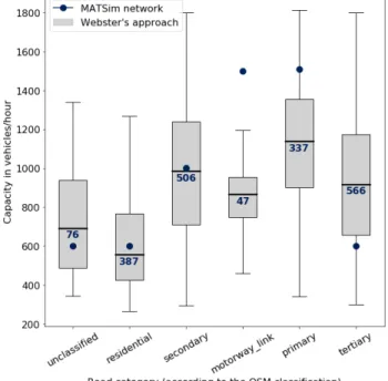
From the figure, one can see that, with Webster’s approach, the capacities are much more 27
diverse than what is assumed in the original Zurich network. For instance, on secondary roads, a 28
default capacity of 1,000 vehicles/hour is assumed. With Webster’s formula, those capacities range 29
approximatively from 300 to 1800 vehicles/hour, which reflects more accurately the diversity of 30
traffic situations that can be observed in reality. One can observe that, on the largest road categories, 31
such as primary and motorway links, the capacity estimates obtained through Webster’s approach 32
are significantly lower than the default values used by MATSim – for more than 50% of primary 33
roads observations, the estimated capacity is smaller than 1150 vehicles/hour whereas a capacity 34
of 1500 vehicles/hour is assumed in the MATSim simulations. This trend is less noticeable on 35
smaller roads. The median road capacities obtained through Webster’s formula for secondary and 36
residential roads are close to the default values used by MATSim. Nonetheless, the opposite trend 37
can be observed on tertiary roads, whose capacities MATSim tends to underestimate (a default 38
capacity of 600 vehicles/hour was assumed, almost 40% less than the observed empirical median 39
which is close to 950 vehicles/hour). Finally, the figure suggests that, regarding the capacities, 40
FIGURE 2: Comparison between capacity estimates obtained through Webster’s approach and the default capacity values assumed in the original MATSim network.
For each road category, the dark blue point indicates the default capacity obtained from OSM. The boxplots illustrate the capacity distributions estimated in this study, depending as well on the road category. The number written in the boxplot is the number of available observations. The default capacity assumed in MATSim for those links is 1,000 vehicles per hour, but the study indicates a capacity median slightly above 600 vehicles/hour.
there is almost no difference between secondary and tertiary roads.
1
From those observations, one can deduce that the default values used in MATSim sim- 2
ulations are not always the most appropriate ones. The employed approach to assign capacities to 3
roads might thus be oversimplistic and should perhaps be adapted to perform simulations that are 4
more consistent with reality. The OSM classification seems to play a major role here as it creates 5
a distinction between secondary and tertiary roads that might not reflect the reality of traffic con- 6
ditions in Zurich. The impacts of those changes in capacities on simulation outputs, such as flow 7
distributions among the network, have however not been examined yet.
8
Consequences on the travel times 9
To compare the travel times in the different simulations, 5,000 origin-destination coor- 10
dinate pairs were generated within the study area. A Java script was then used to compute the 11
optimal route and the corresponding travel times according to simulation outputs, at five different 12
hours of the day (6 a.m., 8 a.m., 12 noon, 6 p.m., 8 p.m.). These different time points correspond 13
to different traffic situations (before the morning peak hours, the morning peak hours itself, day 14
off-peak hours, evening peak hours and after the evening peak hours). Other travel time estimates, 15
for the same origin-destination pairs and for the same periods of the day, were also computed 1
through two web APIs: Google Maps (23) and Bing Maps (24). At the end, for each comparison 2
point (one of the 5,000 origin-destination pairs at one given time), eight travel time estimates were 3
available: six from the various MATSim simulations, one from Google Maps and one from Bing 4
Maps. Using two reference APIs helped to distinguish the differences existing between one online 5
service and MATSim estimates from the bias that one of those two references can have compared 6
to the other – from the results that will be presented, it will be obvious that Google Maps tends to 7
underestimate travel times compared to Bing Maps.
8
Estimates obtained from Google Maps were considered as the reference and the result 9
show the relative difference, in percentage points, between travel times obtained from the simula- 10
tions or from Bing Maps and these reference values. Figure 3 illustrates the impact, in MATSim 11
baseline simulations, of a change in the crossing penalty. Those relative differences were capped 12
in absolute value at 100% for the sake of visibility.
13
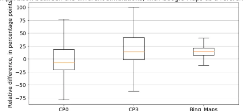
FIGURE 3: Relative difference between travel time estimates in the baseline simulations with crossing penalties equal to 0 (CP0) and 3 seconds (CP3) on the one hand, and estimates from Bing Maps on the other hand, and estimations given by Google Maps as a reference, in percentage points.
From the figure, one can see that the median relative difference increases from -7%
14
in the simulation with zero crossing penalty to 13.9% in the one with a crossing penalty equal 15
to 3 seconds. As the corresponding median from Bing Maps estimates amounts to 14.4%, one 16
understands why the value of 3 seconds was proposed as the default crossing penalty in Zurich:
17
with it, the travel times estimates are as close as possible to the ones provided by this API. However, 18
one can notice that the range between the first and ninth deciles remains unchanged, as well as 19
the range between the first and the third quartiles, when the crossing penalty is modified. Those 20
intervals are however large compared to the ones observed in the results from Bing Maps. With 21
the default crossing penalty, it is neither unlikely to underestimate the travel times by 60% nor to 22
overestimate it by 100% or more, whereas relative differences higher, in absolute value, than 30%, 23
are rare in the results from Bing Maps. To summarize, changing the crossing penalty seems to 24
result only in a translation, upwards or downwards, of the boxplot depicting the relative difference 25
of travel time estimates.
26
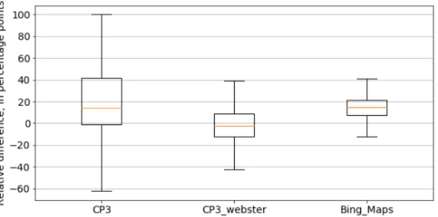
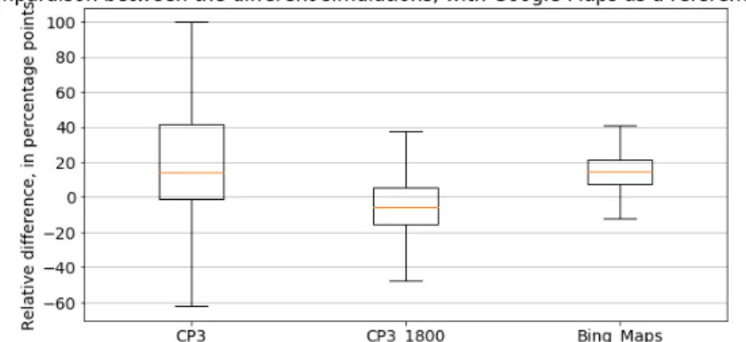
FIGURE 4: Relative difference between travel time estimates in the baseline simulation with crossing penalty equal to 3 seconds (CP3), in the simulation enforcing Webster’s approach with flows coming from the baseline simulation with the same crossing penalty (CP3_Webster) and in estimates from Bing Maps, and estimations given by Google Maps as a reference, in percentage points.
Figure 4 depicts the impacts of enforcing Webster’s approach, while keeping the crossing 1
penalty unchanged. Interestingly, with Webster’s method, the travel times appear to be closer to 2
the estimates provided by Google Maps (with a median relative difference of -2.2%) than to the 3
ones obtained from Bing Maps, contrary to what is observed while only enforcing the crossing 4
penalty. Moreover, one can see that both the interval between the first and ninth decile and the one 5
between the first and third quartile shrink significantly when Webster’s approach is enforced. This 6
implies that, on average, travel time estimates provided with this method are more reliable than the 7
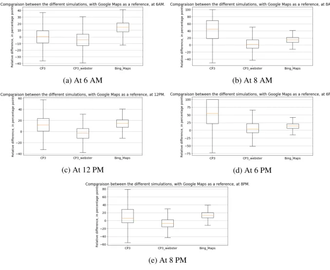
ones obtained with the crossing penalty alone. Figure 5 show the same results split according to 8
the hour when the trip should take place. One can notice that the differences between Webster’s 9
approach and the crossing penalty alone are much more significant at peak hours (8 a.m., 6 p.m.
10
and, to a smaller extent, 8 p.m.) than off peak time (6 a.m. and 12 noon). This observation suggest 11
that enforcing a crossing penalty besides penalizing separately motorists in congestion situations, 12
as it is done in the baseline simulation, might not be the most relevant approach. With Webster’s 13
method, as the computed delay simultaneously comprises the effects of the traffic lights and of 14
congestion, the travel times estimates look more satisfactory, compared to the ones obtained from 15
the two APIs.
16
This suggests that Webster’s approach is not the only reason why simulations implement- 17
ing it provide better estimates than the baseline simulations, and that the road capacities themselves 18
play a prominent role. This is what shows Figure 6, which compares the baseline simulation to 19
the simulation where all link capacities were changed to 1,800 vehicles/hour/lane. The diagramm 20
showing the results of this last simulation is indeed very similar to the one showing results of the 21
simulation with Webster’s approach in Figure 4 – enforcing this approach for a network where no 22
congestion can appear due to capacity limits leads to an increase of the median relative difference 23
of around 3 percentage points.
24
(a) At 6 AM (b) At 8 AM
(c) At 12 PM (d) At 6 PM
(e) At 8 PM
FIGURE 5: Relative difference between travel time estimates in the baseline simulations with crossing penalty equal to 3 seconds (CP3), in the simulation enforcing Webster’s approach with flows coming from the baseline simulation with the same crossing penalty (CP3_Webster) and in estimates from Bing Maps, and estimations given by Google Maps as a reference, in percentage points.
CONCLUSION 1
In this paper, a new approach to take into account traffic lights during MATSim simu- 2
lations was proposed. This method uses Webster’s formula to compute, at the mesoscopic level, 3
the delays experienced by motorists due to traffic signals themselves and queues forming because 4
of them. A technique to extract the traffic lights’ localizations and to integrate them automatically 5
in an already existing MATSim network was also developed and represents another significant 6
contribution.
7
While analyzing results obtained through this new approach, the prominent role of road 8
capacities within MATSim simulations was brought to light. It was shown that the capacities 9
assumed in the default MATSim settings may not be the most appropriate ones to ensure reliable 10
travel time estimates. Moreover, evidence was found that the approach used by default in order 11
FIGURE 6: Relative difference between travel time estimates in the baseline simulation with crossing penalty equal to 3 seconds (CP3), in the same simulation where the link capacities were set to 1,800 vehicles/hour/lane and in estimates from Bing Maps, and estimations given by Google Maps as a reference, in percentage points.
to take into account crossroads, which relies on the manually calibrated crossing penalty, might 1
tend to overpenalize motorists, regarding travel times, in particular at peak hours. On the contrary, 2
the presented method provides reliable travel time estimates, regardless of the hour of the day.
3
Comparing those estimates to the ones provided by microscopic simulation tools, such as SUMO 4
(25), would be worthwhile in order to provide more guarantees about the quality of those estimates.
5
Different parts in the article indicate potential future work. First, Webster’s method is 6
implemented in a static way: final results from one previous simulation are needed to compute the 7
delays that will be enforced, and those delays are not updated iteratively during the simulation to 8
represent the fact that motorists adapt their behavior to them. A dynamic implementation would 9
allow motorists and traffic lights to adapt simultaneously to each other. Secondly, because of this, 10
it is not straightforward to adapt this method to assess the impacts of changes in infrastructure: if 11
a modification is done to the network, a first simulation will have to be performed with the modi- 12
fied network before new delays can be computed and enforced. Besides that, Webster’s approach 13
provides road capacity estimates, it could be interesting to integrate the presented approach in an 14
iterative process, where flows, delays and road capacities could be updated simultaneously.
15
This work showed the drawbacks of the crossing penalty approach, which was employed 16
in MATSim scenarios such as the Zurich scenario. However, the new approach is only suitable for 17
traffic-signaled intersections. In the simulations that were performed for this study, the crossing 18
penalty approach was thus still used for non traffic-signaled intersections. An additional improve- 19
ment would be to propose another method to model in a more accurate way these non traffic- 20
signaled crossroads. Doing so, a complete comparison between the crossing penalty approach and 21
the new one could be performed. The hope is to work in this direction in oder to be soon able 22
to offer a new MATSim module that would model accurately all intersections and thus improve 23
significantly the quality of travel time estimates, when access to detailed traffic signal schedules is 24
not available.
25
AUTHOR CONTRIBUTION 1
The authors confirm contribution to the paper as follows: study conception and design: A. Sallard, 2
M. Bala´c; data collection: A. Sallard; analysis and interpretation of results: A. Sallard, M. Bala´c;
3
draft manuscript preparation: A. Sallard. All authors reviewed the results and approved the final 4
version of the manuscript.
5
REFERENCES
1. Andreas Horni, Kai Nagel, and Kay W. Axhausen. The multi-agent transport simulation MATSim. Ubiquity Press, London, 2016.
2. Dominik Grether. Extension of a multi-agent transport simulation for traffic signal control and air transport systems. PhD thesis, Technische Universität Berlin, 2014.
3. Theresa Thunig, Nico Kühnel, and Kai Nagel. Adaptive traffic signal control for real- world scenarios in agent-based transport simulations. Transportation Research Procedia, 37:481–488, 2019.
4. F. V. Webster. Traffic signal settings. Technical report, 1958.
5. N. Rouphail, A. Tarko, and J. Li. Traffic flow at signalized intersections. 1992.
6. M. Beckman, C. B. McGuire, and C. B. Winsten. Studies in the economics of transporta- tion. 1956.
7. Ding Xin Cheng, Carroll J. Messer, Zong Z. Tian, and Juanyu Liu. Modification of Web- ster’s minimum delay cycle length equation based on HCM 2000. In The 81st Annual Meeting of the Transportation Research Board in Washington, DC, 2003.
8. Alvaro J. Calle-Laguna, Hesham A. Rakha, and P. Eng. Optimizing isolated traffic signal timing considering energy and environmental impacts. Technical report, 2016.
9. Alvaro J. Calle-Laguna, Jianhe Du, and Hesham A. Rakha. Computing optimum traf- fic signal cycle length considering vehicle delay and fuel consumption. Transportation Research Interdisciplinary Perspectives, 3:100021, 2019.
10. TS Babicheva. The use of queuing theory at research and optimization of traffic on the signal-controlled road intersections. Procedia Computer Science, 55:469–478, 2015.
11. Ozan K. Tonguz, Wantanee Viriyasitavat, and Fan Bai. Modeling urban traffic: a cellular automata approach. IEEE Communications Magazine, 47(5):142–150, 2009.
12. Stefan Lämmer and Dirk Helbing. Self-control of traffic lights and vehicle flows in ur- ban road networks. Journal of Statistical Mechanics: Theory and Experiment, 2008(04):
P04019, 2008.
13. Stefan Lämmer and Dirk Helbing. Self-stabilizing decentralized signal control of realistic, saturated network traffic. Santa Fe Institute, 2010.
14. Stefan Lämmer. Selbst-gesteuerte Lichtsignalanlagen im Praxistest (self-controlled traffic signals, an empirical test). Straßenverkehrstechnik, 3:143–151, 2016.
15. Sebastian Hörl. Dynamic Demand Simulation for Automated Mobility on Demand. PhD thesis, ETH Zurich, 2020.
16. Dominik Grether and Theresa Thunig. Traffic signals and lanes. 2016.
17. Sebastian Hörl, Felix Becker, Thibaut J. P. Dubernet, and Kay W. Axhausen. Induzierter Verkehr durch autonome Fahrzeuge: Eine Abschätzung (traffic induced by autonomous vehicles: an estimation). Technical report, ETH Zurich, 2019.
18. Miloš Bala´c and Sebastian Hörl. Eqasim. URLhttps://eqasim.org/.
19. Open street maps. URLhttps://www.openstreetmap.org/.
20. QGIS.org (2020). QGIS geographic information system. Open source geospatial founda- tion project. URLhttps://www.qgis.org/.
21. Aric A. Hagberg, Daniel A. Schult, and Pieter J. Swart. Exploring network structure, dynamics, and function using networkx. In Gaël Varoquaux, Travis Vaught, and Jarrod Millman, editors, Proceedings of the 7th Python in Science Conference, pages 11 – 15, Pasadena, CA USA, 2008.
22. Thomas Riedel and Monica Menendez. Global Practices on Road Traffic Signal Control:
Fixed-time Control at Isolated Intersections. Elsevier, 2019.
23. Google. Google Directions API. URLhttps://www.google.com/maps.
24. Bing. Microsoft Bing Maps Platform API. URLhttps://www.bing.com/maps.
25. Pablo Alvarez Lopez, Michael Behrisch, Laura Bieker-Walz, Jakob Erdmann, Yun-Pang Flötteröd, Robert Hilbrich, Leonhard Lücken, Johannes Rummel, Peter Wagner, and Eva- marie Wießner. Microscopic traffic simulation using SUMO. In The 21st IEEE Inter- national Conference on Intelligent Transportation Systems. IEEE, 2018. URL https:
//elib.dlr.de/124092/.