Send your solutions to this chapter’s tasks until

Prof. Dr. Michael Griebel Prof. Dr. Jochen Garcke Dr. Bastian Bohn Jannik Schürg

5

D E E P N E U R A L N E T WO R K S

Send your solutions to this chapter’s tasks until

July 3rd.

After having considered unsupervised learning methods on sheets 3 and 4, we now come back to supervised learning once more. Recall that we are given data D : = {( x i , y _i ) ∈ _Ω × _Γ | i = 1, . . . , n } drawn i.i.d. according to some measure µ and we are looking for a function f , which approximately achieves f ( x ) = y for ( x, y ) ∼ µ. As before, we tacitely assume Ω ⊂ _R ^d _{and Γ} ⊂ R. We now turn to the model class of (artificial) neural networks and especially deep neural networks (DNN).

This class is very popular in machine learning nowadays and a vast zoo of specific types of DNNs exists, which are used for many different tasks such as speech recognition, automated video sequencing, graph learning or image generation, see e.g. http://www.asimovinstitute.

org/neural-network-zoo/ and [2, 6].

The basic idea of a neural network is to model the way in which infor- mation is propagated between neurons in the human brain. Specifically, they are built on the analogon of sending an electrical signal along a neuron synapse. In an artificial neural network model, certain neurons are connected to each other and - based on the state of a neuron - a signal is passed along these connections to adjacent neurons. Depend- ing on how important a connection is, it is given a certain weight. We will stick here to the class of feedforward networks, which means that information is passed only in one direction.

a single - layer feedforward network

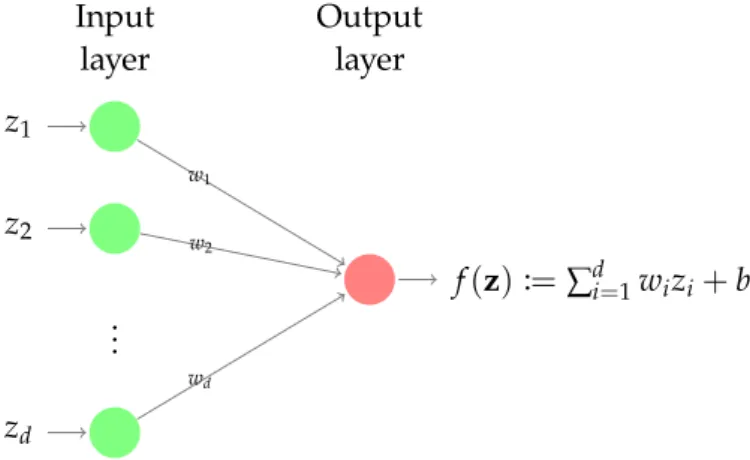
A feedforward neural network can directly be modeled as a specific directed acyclic graph. In the easiest case, we are dealing with a single- layer neural network1, see figure 5.1. For this simple network model, the i -th neuron of the input layer contains the component z _i of an input vector z ∈ _R ^d . Then it propagates this information to the single output layer neuron by multiplying it with the connection weight w _i . At the output neuron, the propagated information of all input neurons is summed up and a bias b is added. The result is

f ( _z ) =

∑ d i =

w _i z _i + b.

1 Note that the output layer is usually not counted. Therefore, we refer to this as a single-

or one-layer neural network.

z

z

.. . z _d

f ( z ) : = _∑ ^d _{i =}

w _i z _i + b

w1

w2

wd

Input layer

Output layer

Figure 5.1: A one-layer neural network, which gets a vector z = ( z

, . . . , z _d ) as input and computes f ( _z ) by propagating it to the output layer.

Viewing the weights w _i for i = 1, . . . , d and the bias b as degrees of freedom, we already know the model class of f very well: This is exactly the class of affine linear functions. Thus, the model class that can be represented by this most simple neural network is the class of affine linear functions. To obtain a classifier, usually a nonlinear activation function φ : R → _R is applied to the result in the output layer. The most simplest one in the case of two classes Γ = { 0, 1 } would be the heaviside function

φ ( t ) = (

1 if t > 0 0 else

for which we obtain the so-called perceptron neural network, which was invented by F. Rosenblatt in 1957, see [11]. It resembles the first step for machine learning with neural networks. While this is a nice fact per se, we already exhaustively dealt with this model class on the first sheets. To create a broader model class, we will now add more layers (so-called hidden layers) in between the input and the output layer to the network.

a two - layer feedforward network

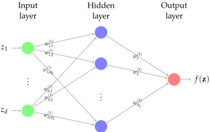
Let us now consider a more involved two-layer network, see figure 5.2. This network consists of an input layer with d

: = d neurons, one hidden layer with d

neurons and an output layer with a single neuron.

For an input z ∈ _R ^d the network does the following:

• Neuron i of the input layer gets the data z _i of the input vector.

• The information z _i is passed on by neuron i of the input layer to

neuron j of the subsequent layer multiplied by the weight w _i,j ⁽

⁾ .

5.2 a two - layer feedforward network 51

z

.. .

z _d

.. .

f ( z )

w⁽¹⁾_1,1 w⁽¹⁾_1,2

w_1,d⁽¹⁾

2

w⁽¹⁾_d,1 w_d,2⁽¹⁾

w⁽¹⁾_d,d

2

w⁽²⁾₁ w⁽²⁾₂

w⁽²⁾_d

2

Hidden layer Input

layer

Output layer

Figure 5.2: A fully-connected two-layer neural network (one hidden layer), which gets a vector z = ( z

, . . . , z _d ) as input and computes f ( z ) by propagating the input through the network architecture. Here, the hidden layer has d

neurons.

• All the information w ⁽ _i,j

⁾ · z _i for all i = 1, . . . , d that arrives in neuron j of the hidden layer is summed up and a bias b ⁽ _j

⁾ is added to create the so-called net sum:

net ⁽ _j

⁾ : =

∑ d i =

w ⁽ _i,j

⁾ z _i + b ⁽ _j

⁾ .

• The net sum is taken as input for an activation function φ ⁽

⁾ : R → _{R. Thus,} o ⁽ _j

⁾ : = φ ⁽

⁾ ( net ⁽ _j

⁾ ) is the information computed (and stored) in neuron j of the hidden layer.

• Now each neuron j of the hidden layer passes its information o ⁽ _j

⁾ to each neuron of the next layer. In our case, this is the output layer, which only consists of a single neuron. Again, the information is multiplied by the corresponding weight w ⁽ _j

⁾ .

• The information that arrives in the output layer is summed up to net ⁽

⁾ : =

d

∑ j =

w ⁽ _j

⁾ o ⁽ _j

⁾ + b ⁽

⁾ ,

where b ⁽

⁾ is the bias of the output neuron.

• We apply a final activation function φ ⁽

⁾ to obtain f ( z ) = o ⁽

⁾ : = φ ⁽

⁾ ( net ⁽

⁾ ) =

= φ ⁽

⁾

d

∑ j =

w ⁽ _j

⁾ · φ ⁽

⁾

∑ d i =

w ⁽ _i,j

⁾ z _i + b ⁽ _j

⁾

! + b ⁽

⁾

!

.

This is called forward propagation of the information/input z and it computes the output f ( z ) according to the neural network f defined by the architecture from figure 5.2. Note that, for regression, we usually choose the final activation function to be φ ⁽

⁾ : = _{id, so} o ⁽

⁾ = net ⁽

⁾ . Obviously, the model class from which f stems is now much more involved than in the single-layer case.

deep neural networks

We can directly see that, the more hidden layers we add to the network, the more involved and complicated the structure of f gets. Networks with more than one hidden layer are usually referred to as deep neural networks.

Computing point evaluations of f – forward propagation

For a given vector z ∈ d , we want to compute f ( _z ) _{, where} f is the function given by the neural network. The generalization from the two-layer case to the L-layer case with L > 2 is straightforward: Given the values o _i ^{( l )} for i = 1, . . . , d _l computed in the neurons of the l-th layer2, we obtain the values in the l + 1-th layer by computing the net sum of the j-th neuron by

net ⁽ _j ^{l +}

⁾ : =

d

i ∑ =

w ⁽ _i,j ^{l )} o ⁽ _i ^{l )} + b ⁽ _j ^{l +}

⁾

and applying the activation function of the l + 1-th layer to get o ⁽ _j ^{l +}

⁾ : = φ ^{( l +}

⁾ ( net ⁽ _j ^{l +}

⁾ ) .

This procedure is then iterated until we reach the output layer. Note that we can also write this in a matrix-vector-fashion

net ~ ^{( l +}

⁾ : = W ^{( l )} T

·~ o ^{( l )} + ~ _b ^{( l +}

⁾

with weight matrix entries W ⁽ _ij ^{l )} : = w ⁽ _i,j ^{l )} . Often - by abusing notation - you will see the application of the activation function written as

~ o ^{( l +}

⁾ : = φ ^{( l +}

⁾ ( _net ~ ^{( l +}

⁾ ) ,

where the application of φ ^{( l +}

⁾ is meant component-wise.

Apart from classic activation functions such as φ ^{( l )} ( z ) = tanh ( z ) or φ ^{( l )} ( z ) =

₊

_e

, the most famous one in recent artificial neural networks is the so-called rectified linear unit or just ReLU-function φ ^{( l )} ( z ) = ReLU ( z ) : = max ( 0, z ) _.

2 For the case l = 1, we just set o

: = z

for i = 1, . . . , d

with d

= _d.

5.3 deep neural networks 53 While deep neural networks have already been studied in the 1960s, their popularity in machine learning emerged only in the last 10 years, due to the fact that adequate hardware and efficient training algorithms to determine the weights and biases have been missing earlier.

Least-squares error minimization

Finally, let us have a look at how to train a neural network, i.e. how to determine the weights and biases. To this end, we will again aim to minimize the least-squares loss function

1 n

∑ n i =

C _i ( f ) : = ¹ n

∑ n i =

( f ( x _i ) − y _i )

_(5.1)

for the neural network model f . For L > 2 the minimization problem is nonlinear and (usually) nonconvex, which makes the mathematical and numerical treatment much harder than in the case of linear mod- els. If a minimizer of (5.1) exists, it is usually not even unique and - for deep networks with large L - many local minimizers exist. Never- theless, many numerical experiments in the last decades have shown that gradient-based minimization algorithms such as quasi-Newton algorithms or even simple descent methods lead to very good results when employed to solve (5.1). Note that we already employed a gra- dient descent algorithm for the most simple neural network model class, namely the affine linear one, on sheet 1. To compute the gradient w.r.t. the weights and biases of (5.1), we will use the so-called backward propagation or backprop algorithm, which is based on the chain rule.

Computing the gradients of C _i – backward propagation

Since the one-point loss C _i for i = 1, . . . , n is just a random instance of C ( f ) : = ( f ( x ) − y )

_for ( x, y ) ∼ µ, we will focus on computing

∂C ( f )

∂w ⁽ _i,j ^{l )} and ∂C ( f )

∂b ⁽ _j ^{l +}

⁾

∀ i = 1, . . . , d _l and j = 1, . . . , d _{l +}

for l = 1, . . . , L.

Note that the chain rule gives us

∂C ( f )

∂w ⁽ _i,j ^{l )}

= ^∂C ( f )

∂o ⁽ _j ^{l +}

⁾

· ^∂o

( l +

) j

∂ net ⁽ _j ^{l +}

⁾

· ^{∂ net}

( l +

) j

∂w _i,j ^{( l )}

= ^∂C ( f )

∂o ⁽ _j ^{l +}

⁾

· φ ^{( l +}

⁾ 0

net ⁽ _j ^{l +}

⁾

· o _i ^{( l )} .

For the first term we have

∂C ( f )

∂o ⁽ _j ^{l +}

⁾

=



 

 

2 ( f ( x ) − y ) _if l = L,

∑ ^d _{i =}

^{( f )}

∂net⁽_i^l+2)

·

(l+2) i

∂o⁽_j^l+1)

else.

Since

(l+2) i

∂o⁽_j^l+1)

= w ⁽ _j,i ^{l +}

⁾ and

∂C ( f )

∂ net ⁽ _i ^{l +}

⁾

= ^∂C ( f )

∂o ⁽ _i ^{l +}

⁾

· ^∂o

( l +

) i

∂ net ⁽ _i ^{l +}

⁾

= ^∂C ( f )

∂o ⁽ _i ^{l +}

⁾

· φ ^{( l +}

⁾ 0

net ⁽ _i ^{l +}

⁾ ,

we can calculate

^{( f )}

∂w⁽_i,j^l)

starting at the final layer and iterate backwards step by step. This process is called backward propagation or simply back- prop. To this end, let us iteratively define

δ ⁽ _j ^{l )} : =







2 ( f ( x ) − y ) = 2 ( o ⁽

^{L +}

⁾ − y ) _if l = L,

∑ ^d _i =

δ ⁽ _i ^{l +}

⁾ · φ ^{( l +}

⁾ 0

net ⁽ _i ^{l +}

⁾

· w ⁽ _j,i ^{l +}

⁾ else.

Then, it follows

∂C ( f )

∂w ⁽ _i,j ^{l )}

= δ _j ^{( l )} · φ ^{( l +}

⁾ 0

net ⁽ _j ^{l +}

⁾

· o ⁽ _i ^{l )}

for l = _{1, . . . ,} L . Analogously, one can show

∂C ( f )

∂b ⁽ _j ^{l +}

⁾

= δ ⁽ _j ^{l )} · φ ^{( l +}

⁾ 0

net ⁽ _j ^{l +}

⁾

.

Again, we can write this down in a matrix-vector format by

~ _δ ^{( l )} _: =







2 ( f ( x ) − y ) _if l = L,

W ^{( l +}

⁾ ·

~ _δ ^{( l +}

⁾ φ ^{( l +}

⁾ 0

net ~ ^{( l +}

⁾ else, which gives us the derivatives

∇

C ( f ) = ~ o ^{( l )} ·

~ _δ ^{( l )} φ ^{( l +}

⁾ 0

net ~ ^{( l +}

⁾ T

∈ _R ^d

^{× d}

_,

∇ _{~ b}

C ( f ) = ~ _δ ^{( l )} φ ^{( l +}

⁾ 0

net ~ ^{( l +}

⁾

∈ _R ^d

, where denotes the Hadamard product.

This shows us, how the derivatives for one data tuple ( _x, y ) _can be computed. Doing this for all ( x _i , y _i ) _with i = 1, . . . , n gives us the derivatives of (5.1) w.r.t. the weights and biases. This enables us to employ a gradient descent algorithm.

Training the network – stochastic (minibatch) gradient descent

Let us now introduce an advanced variant of the gradient descent

optimizer we had on sheet 1. Instead of using a standard gradient

descent optimizer, which can be costly for large data sets, we will use

a stochastic variant, where a subset B ⊂ { 1, . . . , n } is chosen randomly

5.3 deep neural networks 55 in each iteration step and the gradient ∇ _w,b w.r.t. all weights and biases of

C _B ( f ) : = ¹

| B | ∑

i ∈ B

C _i ( f )

is computed instead of the gradient of (5.1). This is much cheaper if

| B | n and gives an unbiased estimate of the gradient of C ( f ) _since the data is drawn i.i.d. according to µ. The overall stochastic minibatch gradient descent algorithm for the minimization of (5.1) is given in algorithm 5.5.

Algorithm 5.5 Stochastic gradient descent algorithm to determine a minimizer of (5.1).

Input: Data set D , learning rate ν > 0, minibatch size K, number of steps S.

for all s = 1, . . . , S do

Draw a random set B ⊂ { 1, . . . , n } _{of size} K . Calculate f ( x _i ) ∀ i ∈ B via forward propagation.

Calculate ∇ _w,b C _B ( f ) via backprop.

Update the weights and biases W ^{( l )} ← W ^{( l )} − ν · ∇

C _B ( f ) _,

~ _b ^{( l +}

) ← ~ _b ^{( l +}

) − ν · ∇ _~

b

C _B ( f ) for all l = 1, . . . , L.

end for

Task 5.1. Implement a class TwoLayerNN , which represents a (fully-connected, feed-forward) two-layer neural network, i.e. L = 2 . The activation functions should be φ ⁽

⁾ = ReLU and φ ⁽

⁾ = id . The weights and biases can be ini- tialized by drawing i.i.d. uniformly distributed random numbers in (− 1, 1 ) _. The class should contain a method feedForward to calculate the point evalu- ations of f for a whole minibatch at once and a method backprop to calculate

∇ _w,b C _B ( f ) . To this end, avoid using for-loops over the minibatch and use linear algebra operations (on vectors, matrices or tensors) instead.

Task 5.2. Augment the TwoLayerNN class by implementing methods to ran- domly draw a minibatch data set and a method to perform the stochastic minibatch gradient descent algorithm.

Task 5.3. Test your implementation by drawing 250 uniformly distributed

points x _i in R

with norm k x _i k ≤ 1 and label them by y _i = − 1 . Now draw

250 uniformly distributed points x i in R

with 1 < k _{x i} k ≤ 2 and label them

by y _i = 1 . Use your two-Layer neural network with d

= 20 hidden layer

neurons, S = 50000 iterations and K = 20 to classify the data. Try different

learning rates ν . Output the least-squares error every 5000 iterations. After

S iterations, make a scatter plot of the data and draw the contour line of your

learned classifier. What do you observe? What happens if you increase S ?

z

z

z

z

z

z

max

max

max

c1

c2

c3

c1

c2

c3

c1

c2

c3

c1

c2

c3

c2

c2

c3

c1

Convolutional layer

Input layer

Pooling layer

Figure 5.3: A convolutional layer with three (shared) weights c

, c

, c

applied

to z = ( z

, . . . , z

) followed by a downsampling/max-pooling

layer with 3 neurons.

relation to other methods / models

Finally, let us remark some analogies of (deep) neural networks to other models/methods.

A relation to kernel methods

While the weights and the biases are degrees of freedom of our model class, the (possibly nonlinear) activation functions φ ^{( l )} are usually fixed a priori. Let φ ^{( L +}

⁾ = id. Since we are only dealing with a single output neuron, we can rewrite our model as

f ( z ) = ~ w ^{( L )} T

· ψ ( z ) + b ^{( L +}

⁾

for a vector-valued function ψ : R ^d → _R ^d

depending on the weights, biases and activation functions of the previous l = 1, . . . , L − 1 layers.

In this way, we have a direct analogy to SVM or kernel methods in general, where ψ reflects the feature map which is chosen to transform the data. However, the difference between the SVM and the hidden- layer neural network model is that ψ—or equivalently the kernel K—

has been chosen a priori for SVM, whereas here ψ depends on the

degrees of freedom (namely the weights and biases of the hidden

5.5 convolutional neural networks 57 layers). Furthermore, there also exist hybrids between kernel methods and deep neural networks called deep kernel networks, see e.g. [1].

A relation to ordinary differential equations (ODEs)

A special class of neural networks are so-called residual networks (ResNets).

Here, the forward propagation step can be written in the form

~ o ^{( l +}

⁾ = ~ o ^{( l )} + _∆t · φ ^{( l +}

⁾

W ^{( l )} T

·~ o ^{( l )} + ~ _b ^{( l +}

⁾

,

where ∆ t > 0 is some positive scaling parameter. If we assume that the activation function is the same in each iteration step, this can be written as

~ _o ^{( l +}

⁾ − ~ _o ^{( l )}

∆t = φ

W ^{( l )} T

·~ o ^{( l )} + ~ _b ^{( l +}

⁾

. (5.2)

Therefore, we can reinterpret this as a time-explicit Euler discretization with step width ∆ t for the ODE

~ o ˙ ( t ) = φ

W ^T ( t ) ~ o ( t ) + ~ _b ( t ) . (5.3) Therefore, a stable forward propagation can only be guaranteed if the ODE itself admits stable solutions. From ODE theory, it is well-known that this holds if the real part of the eigenvalues of the Jacobian J of the RHS of (5.3) are non-positive. Furthermore, it is needed that the explicit Euler scheme is stable, which holds if

| 1 + _∆ t · λ _i ( _J ^{( l )} )| ≤ 1 ∀ l = 1, . . . , L − 1

is fulfilled for all eigenvalues λ _i ( J ^{( l )} ) _{of the} l-th layer Jacobian J ^{( l )} of the RHS of (5.2). This reinterpretation motivates the creation of new forms of neural networks which allow for stable evaluations, e.g.

Hamiltonian-based networks with a leapfrog-type discretization, see [7].

convolutional neural networks

By many experts, the breakthrough in deep learning is considered to be a model published in 2012. It was submitted to the ImageNet Large Scale Visual Recognition Challenge3 (ILSVRC) by a team around Alex

In the literature the model is referred to as AlexNet.

Krizhevsky [8]. One remarkable observation about this model is, that it used a machine learning technique which was not very popular at that time. Therefore, none of the other entries did use it. The second

3 An annual challenge using a dataset of 1.2 million images from various sources. Each

image depicts objects from 1000 categories which were hand–labeled using Amazon

Turk. The collection of the ImageNet dataset is a great achievement by itself.

remarkable thing is, that it did beat its competitors by over ten percent points4 in the error rate.

The model is built using a class of neural networks called (Deep) Convolutional Neural Networks (DCNN), which we will focus on in this section.

When using the HoG features in section 3.4.1 we saw that the dif- ferentiation could be implemented using an image convolution with a kernel matrix. In a CNN such convolutions are used as layers in a neu- ral network. While the weights for the convolution in the HoG features were chosen by hand, the weights in a CNN are free parameters and therefore subject to change during training.

For example, let c

, . . . , c

+

denote weights, and suppose we have d input nodes z

, . . . , z _d . If the first hidden layer is a convolutional layer its inputs are computed by

net ⁽ _j

⁾ : =

∑ n k =− n

z _{j + k} c _{n +}

_{− k}

where the values z _l for l > d or l < 1 are set to zero. In this way, weights are shared in comparison to a fully-connected layer as previously described. An example for d = 6 and n = 1 is depicted in figure 5.3. Usually more than one convolutional layer is used in parallel, resulting in a multidimensional output. Also, the input dimension can be arbitrary.

CNNs are especially popular for images. While we previously flat- tened the image and used, for example, the pixels row-wise as input to a classifier, we can now keep the 2D representation. The advantage is that locality information is available to the net in this way.

In many cases a stack of convolutional layers is used at the beginning of a network to learn features. Here, one expects the layers to learn higher and higher abstractions

This can be observed

empirically. down the network. For example one

convolution at the beginning might encode lines in certain directions, another one encodes circles, while deeper layers use these pieces of information to recognize, say, body parts.

A certain type of activation functions is usually used for convolu- tional layers. Here, a technique called subsampling is employed. The idea is to apply a function to the convolution outputs in order to make the network invariant under certain transformations. For example, the common max-pooling selects the maximum values among all (possibly overlapping) square regions of given size. In this way the network is expected to be stable under small translations. Other options are for example `

_or `

averages. A neat side effect is that this decreases the number of neurons if the regions do not overlap too much. In practice max-pooling is implemented as an additional layer, see figure 5.3 for a non-overlapping max-pooling example.

4 The results can be found here: http://www.image-net.org/challenges/LSVRC/

2012/results.html .

5.5 convolutional neural networks 59 After applying some convolutional layers, the input is often flat- tened into a one-dimensional feature vector and then fed into a final fully-connected layer for an M-class classification problem (M = | _Γ | _).

The output layer is then made of M nodes, representing a probability

distribution The labels are also

expected to be in this form.

. This is achieved for example by the softmax activation function,

o ⁽ _j ^{L +}

⁾ : =

exp

net ⁽ _j ^{L +}

⁾

∑ _i ^d =

exp

net ⁽ _i ^{L +}

⁾ ,

where d _L +

= M .

Finally, a suitable choice has to be made for the loss function (opti- mization objective). Matching the softmax function, log-likelihood is a popular choice leading to maximum likelihood estimation (MLE)

max w,b

∑ M i =

log ( _P [ y _i | x _i , w, b ]) .

We will use the so called cross entropy loss, which is related to MLE.

Keras

For the final tasks we use the K eras library [4]. It provides a high-level and easy to use abstraction for popular deep learning backends such as Tensorflow.

Defining the network from task 5.3 could be done like this import keras

import keras . layers as layers model = keras . models . Sequential ()

model . add ( layers . Dense (20 , input_shape =(2 ,) , activation =’ relu ’))

model . add ( layers . Dense (1) )

You can print a summary with print(model.summary()) .

Continue with compiling the model ^mse stands for mean

squared error, cf.

eq. (5.1), sgd is an abbreviation for algorithm 5.5.

model . compile ( loss =’mse ’, optimizer = ’sgd ’, metrics =[’ accuracy ’])

and then start training by K = 20

S = 50000

history = model . fit ( X_train , Y_train , batch_size =K , epochs =S / (500 / K) ,

verbose = True )

The gradient implementation5 is derived using automatic differentia- tion. In contrast to numeric differentiation (derivative approximated,

5 The network is at least piece-wise differentiable.

e.g. by computing the difference quotient) here the symbolic knowl- edge about the network is used. This works similar to a computer algebra system (CAS) like Mathmematica, Maple, Octave, etc.

K eras has support for several gradient descent variants, which can also be configured (e.g. change step size). Of course, the final layer can have an activation function too, e.g. softmax when used for classifica- tion.

A convolutional layer with a ReLU activation can be added with model . add ( layers . Conv2D (16 , kernel_size =(3 , 3) ,

activation =’ relu ’))

which adds 16 parallel layers (i.e. 16 layers of the same shape at the same position6) each with a 3 × 3 convolutional matrix for 2D input.

To flatten the result for classification use model . add ( layers . Flatten () )

Regularization

To prevent over-fitting many techniques are known, but most of them are not well understood. A very popular technique is called dropout, where – during each training step – one neglects nodes in a layer with a given probability p. In this way, random sub-nets are trained. To add dropout regularization to a layer use

model . add ( layers . Dropout (p)) after it.

Keras also has support for using regularization terms in the loss function, similar to what we have seen when discussing SVMs.

Task 5.4. Use K eras to build a classifier for the MNIST dataset (see template notebook).

(a) Build a model with the following layers:

– Fully-connected layer ( Dense ) with 128 output nodes + ReLU.

– Fully-connected layer with 128 output nodes + ReLU.

– Fully-connected layer with 10 output nodes + softmax.

Use the SGD optimizer with a batch size of 128 and the categorical crossentropy loss ( loss="categorical_crossentropy" ), train for 20 episodes. Use the accuracy metric (set in model.compile ) and provide the test data as validation data to model.fit (set the parameter validation_data to (X_test, Y_test) ). Plot the fit history (return value of model.fit ).

(b) Build a new network by adding dropout ( p = 0.3 ) to the first and second layer of the model from (a). Train it for 250 episodes.

6 This can also be understood in the following way: Each neuron of the convolutional

layer contains a sixteen-dimensional vector.

5.6 outlook 61 (c) Build a third network by using the model from (b) with the optimizer

"adam" instead of SGD. Be prepared to roughly explain what this optimizer does. Train for 20 episodes.

Task 5.5. Build a CNN with K eras with the following layers:

• 16 parallel conv. layer with kernel size 3 × 3 + ReLU.

• 32 parallel conv. layer with kernel size 3 × 3 + ReLU.

• A 2D max pooling layer of size 2 × 2 , non-overlapping + dropout ( p = 0.25 ).

• Flatten + fully-connected layer with 128 outputs + ReLU + dropout ( p = _0.5)

• Fully-connected layer with output size 10 + softmax.

Train for 15 episodes, the other parameters should be the same as in the previous model.

Feel free to change the network/training in order to improve the error.

Task 5.6. (Bonus) Use a CNN to learn features for pedestrian classification.

Proceed as follows:

• Design and train a CNN for pedestrian classification (use the data from section 3.4). You can start with the network from task 5.5.

• Use the output after the flattening (see K eras ’ FAQ on how to do this) as a feature vector for a linear SVM, together with the HoG features.

Try to use PCA in order to improve the accuracy, also tweak the HoG parame- ters. Make sure not to over-fit (the pedestrian dataset is small in deep learning standards). You can also install the A ugmentor library for P ython in order to enlarge the dataset (common technique in deep learning). We did obtain a 93.5% error rate, but there is definitely room for improvement! You might also want to take a look at the images which got classified wrongly.

outlook

gpus Keras (more precisely its backends) can take advantage of a

GPU (graphics card) in order to speed up the training. If you did the

tasks your training was probably using the CPU, even if your machine

has a GPU. Setting this up can be challenging. But if successful, the

performance gain is usually significant. We did run task 5.5 on six Xeon

3.6 GHz (Sandy Bridge) cores and on a Tesla P100 GPU. For the CPU

one episode of training took 30 seconds (a 2012 Quad-Core laptop took

over a minute), while on the GPU an episode was finished in three

seconds. Even higher speedups are common (our network is probably

too small).

Training a neural network is a lot of try-and-error and needs experi- ence and patience. Modern networks can only be trained (in reasonable time) on a GPU or dedicated hardware. For example, AlexNet had 60 million parameters and was trained over six days on two GPUs.

references on general neural networks and cnns For further programming resources the free course at fast.ai7 could be interesting. See also the book [6] or the review [10] on CNNs. There you will also find references to attempts on describing the history of neural networks.

adversarial neural networks Another interesting branch of literature is the one on attacks against neural networks. For example [3]

designed a sticker that you can patch onto (or near) objects to make a CNN classify everything as a toaster.8 In [5] the authors investigate how robust a CNN can detect traffic stop signs when the sign has graffiti on it (“stop eating animals” or fake SOP signs). Finally, [9] provides examples for manipulated but visually indistinguishable images of traffic signs which get classified differently by a CNN.

references

[1] B. Bohn, M. Griebel, and C. Rieger. “A representer theorem for deep kernel learning.” In: Computing Research Repository (2017).

arXiv: 1709.10441 .

[2] M. Bronstein, J. Bruna, Y. LeCun, A. Szlam, and P. Vandergheynst.

“Geometric deep learning: going beyond Euclidean data.” In:

IEEE Signal Processing Magazine 34 (4 2017), pp. 18–42.

[3] Tom B Brown, Dandelion Mané, Aurko Roy, Martín Abadi, and Justin Gilmer. “Adversarial patch.” In: arXiv preprint arXiv:1712.09665 (2017).

[4] François Chollet et al. Keras. https://keras.io . 2015.

[5] Ivan Evtimov, Kevin Eykholt, Earlence Fernandes, Tadayoshi Kohno, Bo Li, Atul Prakash, Amir Rahmati, and Dawn Song.

“Robust Physical-World Attacks on Deep Learning Models.” In:

arXiv preprint arXiv:1707.08945 1 (2017).

[6] I. Goodfellow, Y. Bengio, and A. Courville. Deep Learning. http:

//www.deeplearningbook.org . MIT Press, 2016.

[7] Eldad Haber and Lars Ruthotto. “Stable architectures for deep neural networks.” In: Inverse Problems 34.1 (2018). 014004.

7 http://www.fast.ai/

8 A top Reddit comment argues that the CNN rightfully does so, and that, in fact, the

sticker does look like a toaster...or a Hunter S. Thompson version of a toaster.

References 63 [8] Alex Krizhevsky, Ilya Sutskever, and Geoffrey E Hinton. “Ima-

genet classification with deep convolutional neural networks.”

In: Advances in neural information processing systems. 2012, pp. 1097–

1105.

[9] Nicolas Papernot, Patrick McDaniel, Ian Goodfellow, Somesh Jha, Z Berkay Celik, and Ananthram Swami. “Practical black- box attacks against deep learning systems using adversarial ex- amples.” In: arXiv preprint (2016).

[10] Waseem Rawat and Zenghui Wang. “Deep convolutional neural networks for image classification: A comprehensive review.” In:

Neural computation 29.9 (2017), pp. 2352–2449.

[11] F. Rosenblatt. “The perceptron: a probabilistic model for infor-

mation storage and organization in the brain.” In: Psychological

Reviews 65 (1958), pp. 386–408.