Reversible Architectures for Arbitrarily Deep Residual Neural Networks

(1)

Reversible Architectures for Arbitrarily Deep Residual Neural Networks

Bo Chang

^∗1,2

, Lili Meng

^∗1,2

, Eldad Haber

^1,2

, Lars Ruthotto

^2,3

, David Begert

²

and Elliot Holtham

²

1University of British Columbia, Vancouver, Canada. (bchang@stat.ubc.ca, menglili@cs.ubc.ca, haber@math.ubc.ca)

2Xtract Technologies Inc., Vancouver, Canada. (david@xtract.ai, elliot@xtract.ai)

3Emory University, Atlanta, USA. (lruthotto@emory.edu). This author is supported in part by NSF DMS 1522599.

∗Authors contributed equally.

Abstract

Recently, deep residual networks have been successfully applied in many computer vision and natural language processing tasks, pushing the state-of-the-art performance with deeper and wider architectures. In this work, we interpret deep residual networks as ordinary differential equations (ODEs), which have long been studied in mathematics and physics with rich theoretical and empirical success. From this interpretation, we develop a theoretical framework on stability and reversibility of deep neural networks, and derive three reversible neural network architectures that can go arbitrarily deep in theory. The reversibility property allows a memory- efficient implementation, which does not need to store the activations for most hidden layers. Together with the stability of our architectures, this enables training deeper networks using only modest computational resources. We provide both theoretical analyses and empirical results. Experimental results demonstrate the efficacy of our architectures against several strong baselines on CIFAR-10, CIFAR-100 and STL-10 with superior or on-par state-of-the-art performance. Furthermore, we show our architectures yield superior results when trained using fewer training data.

1 Introduction

Deep learning powers many research areas and impacts various aspects of society (LeCun, Bengio, and Hinton 2015) from computer vision (He et al. 2016; Huang et al. 2017), natural language processing (Cho et al. 2014) to biology (Es- teva et al. 2017) and e-commerce. Recent progress in designing architectures for deep networks has further accelerated this trend (Simonyan and Zisserman 2015; He et al. 2016;

Huang et al. 2017). Among the most successful architectures are deep residual network (ResNet) and its variants, which are widely used in many computer vision applications (He et al. 2016; Pohlen et al. 2017) and natural language processing tasks (Oord et al. 2016; Xiong et al. 2017;

Wu et al. 2016). However, there still are few theoretical analyses and guidelines for designing and training ResNet.

In contrast to the recent interest in deep residual networks, system of Ordinary Differential Equations (ODEs), special kinds of dynamical systems, have long been studied in mathematics and physics with rich theoretical and empirical Copyright c2018, Association for the Advancement of Artificial Intelligence (www.aaai.org). All rights reserved.

success (Coddington and Levinson 1955; Simmons 2016;

Arnold 2012). The connection between nonlinear ODEs and deep ResNets has been established in the recent works of (E 2017; Haber and Ruthotto 2017; Haber, Ruthotto, and Holtham 2017; Lu et al. 2017; Long et al. 2017; Chang et al. 2017). The continuous interpretation of ResNets as dynamical systems allows the adaption of existing theory and numerical techniques for ODEs to deep learning. For example, the paper (Haber and Ruthotto 2017) introduces the concept of stable networks that can be arbitrarily long. How- ever, only deep networks with simple single-layer convolution building blocks are proposed, and the architectures are not reversible (and thus the length of the network is limited by the amount of available memory), and only simple numerical examples are provided. Our work aims at over- coming these drawbacks and further investigates the efficacy and practicability of stable architectures derived from the dynamical systems perspective.

In this work, we connect deep ResNets and ODEs more closely and propose three stable and reversible architectures.

We show that the three architectures are governed by stable and well-posed ODEs. In particular, our approach allows to train arbitrarily long networks using only minimal memory storage. We illustrate the intrinsic reversibility of these architectures with both theoretical analysis and empirical results. The reversibility property easily leads to a memory- efficient implementation, which does not need to store the activations at most hidden layers. Together with the stability, this allows one to train almost arbitrarily deep architectures using modest computational resources.

The remainder of our paper is organized as follows. We discuss related work in Sec. 2. In Sec. 3 we review the notion of reversibility and stability in ResNets, present three new architectures, and a regularization functional. In Sec. 4 we show the efficacy of our networks using three common classification benchmarks (CIFAR-10, CIFAR-100, STL-10).

Our new architectures achieve comparable or even superior accuracy and, in particular, generalize better when a limited number of labeled training data is used. In Sec. 5 we con- clude the paper.

arXiv:1709.03698v2 [cs.CV] 18 Nov 2017

(2)

Convolution K1

Bias ReLU Convolution K1T

Convolution K2T

Bias ReLU

Convolution K2

+ -

z

y

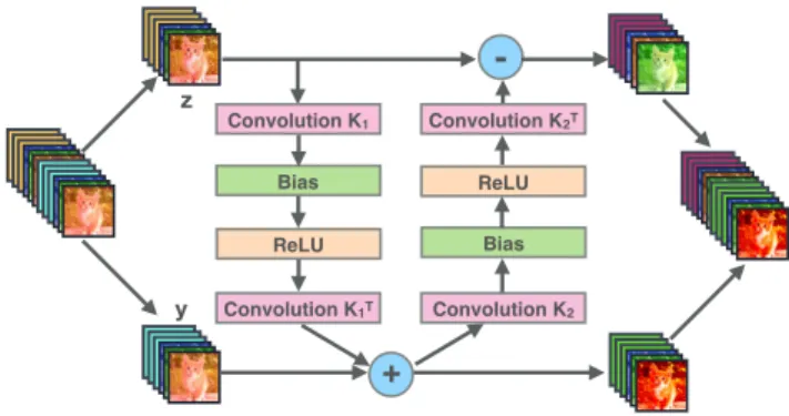
Figure 1:The Hamiltonian Reversible Block.First, the input feature map is equally channel-wise split toY_j andZ_j. Then the operations described in Eq. 10 are performed, re- sulting inY_j+1andZ_j+1. Finally,Y_j+1andZ_j+1are con- catenated as the output of the block.

2 Related Work Residual Neural Networks and Extensions

ResNets are deep neural networks obtained by stacking simple residual blocks (He et al. 2016). A simple residual network block can be written as

Yj+1=Yj+F(Yj,θj) for j= 0, ..., N−1. (1) Here,Y_jare the values of the features at thejth layer andθ_j are thejth layer’s network parameters. The goal of the training is to learn the network parametersθ. Eq. (1) represents a discrete dynamical system. An early review on neural networks as dynamical systems is presented in (Cessac 2010).

ResNets have been broadly applied in many domains including computer vision tasks such as image recognition (He et al. 2016), object detection (He et al. 2017), semantic seg- mentation (Pohlen et al. 2017) and visual reasoning (Perez et al. 2017), natural language processing tasks such as speech synthesis (Oord et al. 2016), speech recognition (Xiong et al. 2017) and machine translation (Wu et al. 2016).

Besides broadening the application domain, some ResNet successors focus on improving accuracy (Xie et al. 2017;

Zagoruyko and Komodakis 2016) and stability (Haber and Ruthotto 2017), saving GPU memory (Gomez et al. 2017), and accelerating the training process (Huang et al. 2016).

For instance, ResNxt (Xie et al. 2017) introduces a homo- geneous, multi-branch architecture to increase the accuracy.

Stochastic depth (Huang et al. 2016) reduces the training time while increases accuracy by randomly dropping a subset of layers and bypassing them with identity function.

Systems of Ordinary Differential Equations

To see the connection between ResNet and ODE systems we add a hyperparameterh > 0to Eq. (1) and rewrite the equation as

Y_j+1−Y_j

h =F(Yj,θ_j). (2)

For a sufficiently smallh, Eq. (2) is a forward Euler discretization of the initial value problem

Y(t) =˙ F(Y(t),θ(t)), Y(0) =Y0. (3)

Thus, the problem of learning the network parameters,θ, is equivalent to solving a parameter estimation problem or op- timal control problem involving the ODE system Eq. (3).

In some cases (e.g., in image classification), Eq. (3) can be interpreted as a system of Partial Differential Equations (PDEs). Such problems have rich theoretical and computational framework, including techniques to guarantee stable networks by using appropriate functionsF, the discretization of the forward propagation process (Ascher and Petzold 1998; Ascher 2010; Bellman 1953), theoretical frameworks for the optimization over the parameters θ (Bock 1983;

Ulbrich 2002; Gunzburger 2003), and methods for com- puting the gradient of the solution with respect toθ (Bliss 1919).

Reversible Architectures

Reversible numerical methods for dynamical systems allow the simulation of the dynamic going from the final time to the initial time, and vice versa. Reversible numerical methods are commonly used in the context of hyperbolic PDEs, where various methods have been proposed and compared (Nguyen and McMechan 2014). The theoretical framework for reversible methods is strongly tied to issues of stability. In fact, as we show here, not every method that is algebraically reversible is numerically stable. This has a strong implication for the practical applicability of reversible methods to deep neural networks.

Recently, various reversible neural networks have been proposed for different purposes and based on different architectures. Recent work by (Dosovitskiy and Brox 2016;

Mahendran and Vedaldi 2015) inverts the feed-forward net and reproduces the input features from their values at the final layers. This suggests that some deep neural networks are reversible: the generative model is just the reverse of the feed-forward net (Arora, Liang, and Ma 2016). (Gilbert et al. 2017) provide a theoretical connection between a model-based compressive sensing and CNNs. NICE (Dinh, Krueger, and Bengio 2015; Dinh, Sohl-Dickstein, and Ben- gio 2016) uses an invertible non-linear transformation to map the data distribution into a latent space where the result- ing distribution factorizes, yielding good generative models.

Besides the implications that reversibility has on the deep generative models, the property can be used for developing memory-efficient algorithms. For instance, RevNet (Gomez et al. 2017), which is inspired by NICE, develops a vari- ant of ResNet where each layer’s activations can be recon- structed from next layer’s. This allows one to avoid storing activations at all hidden layers, except at those layers with stride larger than one. We will show later that our physically- inspired network architectures also have the reversible property and we derive memory-efficient implementations.

3 Methods

We introduce three new reversible architectures for deep neural networks and discuss their stability. We capitalize on the link between ResNets and ODEs to guarantee stability of the forward propagation process and the well-posedness of the learning problem. Finally, we present regularization functionals that favor smooth time dynamics.

(3)

ResNet as an ODE

Eq. (3) interprets ResNet as a discretization of a differential equation, whose parametersθare learned in the training process. The process of forward propagation can be viewed as simulating the nonlinear dynamics that take the initial data, Y0, which are hard to classify, and moves them to a final stateYN, which can be classified easily using, e.g., a linear classifier.

A fundamental question that needs to be addressed is, under what conditions is forward propagation well-posed?

This question is important for two main reasons. First, instability of the forward propagation means that the solution is highly sensitive to data perturbation (e.g., image noise or adversarial attacks). Given that most computations are done in single precision, this may cause serious artifacts and in- stabilities in the final results. Second, training unstable networks may be very difficult in practice and, although impos- sible to prove, instability can add many local minima.

Let us first review the issue of stability. A dynamical system is stable if a small change in the input data leads to a small change in the final result. To better characterize this, assume a small perturbation,δY(0)to the initial dataY(0) in Eq. (3). Assume that this change is propagated through- out the network.The question is, what would be the change after some timet, that is, what isδY(t)?

This change can be characterized by the Lyapunov exponent (Lyapunov 1992), which measures the difference in the trajectories of a nonlinear dynamical system given the initial conditions. The Lyapunov exponent,λ, is defined as the exponent that measures the difference:

kδY(t)k ≈exp(λt)kδY(0)k. (4) The forward propagation is well-posed when λ ≤ 0, and ill-posed ifλ > 0. A bound on the value ofλcan be derived from the eigenvalues of the Jacobian matrix ofFwith respect toY, which is given by

J(t) =∇_Y(t)F(Y(t)).

A sufficient condition for stability is max

i=1,2,...,nRe(λi(J(t)))≤0, ∀t∈[0, T], (5) whereλ_i(J)is the ith eigenvalue ofJ, andRe(·)denotes the real part.

This observation allows us to generate networks that are guaranteed to be stable. It should be emphasized that the stability of the forward propagation is necessary to obtain stable networks that generalize well, but not sufficient. In fact, if the real parts of the eigenvalues in Eq. (5) are negative and large, λ 0, Eq. (4) shows that differences in the input features decay exponentially in time. This compli- cates the learning problem and therefore we consider architectures that lead to Jacobians with (approximately) purely imaginary eigenvalues. We now discuss three such networks that are inspired by different physical interpretations.

The two-layer Hamiltonian network

(Haber and Ruthotto 2017) propose a neural network architecture inspired by Hamiltonian systems

Y(t) =˙ σ(K(t)Z(t) +b(t)),

Z(t) =˙ −σ(K(t)^TY(t) +b(t)), (6) whereY(t)andZ(t)are partitions of the features,σis an activation function, and the network parameters are θ = (K,b). For convolutional neural networks,K(t)andK(t)^T are convolution operator and convolution transpose operator respectively. It can be shown that the Jacobian matrix of this ODE satisfies the condition in Eq. (5), thus it is stable and well-posed. The authors also demonstrate the performance on a small dataset. However, in our numerical experiments we have found that the representability of this “one-layer”

architecture is limited.

According to the universal approximation theorem (Hornik 1991), a two-layer neural network can approxi- mate any monotonically-increasing continuous function on a compact set. Recent work (Zhang et al. 2017) shows that simple two-layer neural networks already have perfect finite sample expressivity as soon as the number of parameters ex- ceeds the number of data points. Therefore, we propose to extend Eq. (6) to the following two-layer structure:

Y(t) =˙ K^T₁(t)σ(K1(t)Z(t) +b1(t)),

Z(t) =˙ −K^T₂(t)σ(K2(t)Y(t) +b2(t)). (7) In principle, any linear operator can be used within the Hamiltonian framework. However, since our numerical experiments consider images, we choose Ki to be a convolution operator, K^T_i as its transpose. Rewriting Eq. (7) in matrix form gives

Y˙ Z˙

=

K^T₁ 0 0 −K^T₂

σ

0 K1

K2 0 Y Z

+ b1

b2

. (8) There are different ways of partitioning the input features, including checkerboard partition and channel-wise partition (Dinh, Sohl-Dickstein, and Bengio 2016). In this work, we use equal channel-wise partition, that is, the first half of the channels of the input isYand the second half isZ.

It can be shown that the Jacobian matrix of Eq. (8) satisfies the condition in Eq. (5), that is,

J=∇(^YZ)

K^T₁ 0 0 −K^T₂

σ

0 K1

K₂ 0 y z

=

K^T₁ 0 0 −K^T₂

diag(σ⁰)

0 K1

K₂ 0

, (9)

wherediag(σ⁰)is the derivative of the activation function.

The eigenvalues of Jare all imaginary (see the Appendix for a proof). Therefore Eq. (5) is satisfied and the forward propagation of our neural network is stable and well-posed.

A commonly used discretization technique for Hamilto- nian systems such as Eq. (7) is the Verlet method (Ascher and Petzold 1998) that reads

Y_j+1=Y_j+hK^T_j1σ(K_j1Z_j+b_j1),

Z_j+1=Z_j−hK^T_j2σ(K_j2Y_j+1+b_j2). (10)

(4)

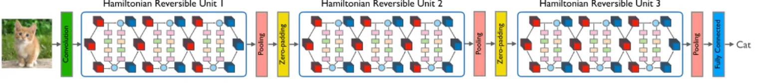
We choose Eq. (10) to be our Hamiltonian blocks and illustrate it in Fig. 1. Similar to ResNet (He et al. 2016), our Hamiltonian reversible network is built by first concatenating blocks to units, and then concatenating units to a network. An illustration of our architecture is provided in Fig. 2.

The midpoint network

Another reversible numerical method for discretizing the first-order ODE in Eq. (3) is obtained by using central finite differences in time

Y_j+1−Y_j−1

2h =F(Y_j). (11)

This gives the following forward propagation

Yj+1=Y_j−1+ 2hF(Yj), for j= 1, . . . , N −1, (12) whereY1is obtained by one forward Euler step. To guarantee stability for a single layer we can use the functionFto contain an anti-symmetric linear operator, that is,

F(Y) =σ((K−K^T)Y+b). (13) The Jacobian of this forward propagation is

J= diag(σ⁰)(K−K^T), (14) which has only imaginary eigenvalues. This yields the single layer midpoint network

Yj+1 =

(2hσ((Kj−K^T_j)Yj+bj), j = 0,

Y_j−1+ 2hσ((Kj−K^T_j)Yj+bj), j>0.

(15) As we see next, it is straightforward to show that the midpoint method is reversible (at least algebraically). However, while it is possible to potentially use a double layer midpoint network, it is difficult to ensure the stability of such network.

To this end, we explore the leapfrog network next.

The leapfrog network

A stable leapfrog network can be seen as a special case of the Hamiltonian network in Eq. (7) when one of the kernels is the identity matrix and one of the activation is the identity function. The leapfrog network involves two derivatives in time and reads

Y(t) =¨ −K(t)^Tσ(K(t)Y(t)+b(t)), Y(0) =Y0. (16) It can be discretized, for example, using the conservative leapfrog discretization, which uses the following symmetric approximation to the second derivative in time

Y(t¨ j)≈h⁻²(Yj+1−2Yj+Yj−1).

Substituting the approximation in Eq. (16), we obtain:

Y_j+1=

(2Yj−h²K^T_jσ(KjYj+bj), j= 0,

2Yj−Y_j−1−h²K^T_jσ(KjYj+bj), j >0.

(17)

Reversible architectures and stability

An architecture is called reversible if it allows the recon- struction of the activations going from the end to the beginning. Reversible numerical methods for ODEs have been studied in the context of hyperbolic differential equations (Nguyen and McMechan 2014), and reversibility was dis- covered recently in the machine learning community (Dinh, Krueger, and Bengio 2015; Gomez et al. 2017). Reversible techniques enable memory-efficient implementations of the network that requires the storage of the last activations only.

Let us first demonstrate the reversibility of the leapfrog network. Assume that we are given the last two states,Y_N and Y_N−1. Then, using Eq. (17) it is straight-forward to computeY_N₋₂:

YN−2= 2YN−1−YN

−h²K^T_N−1σ(KN−1YN−1+b_N−1). (18) GivenYN−2 one can continue and re-compute the activations at each hidden layer during backpropagation. Simi- larly, it is straightforward to show that the midpoint network is reversible.

The Hamiltonian network is similar to the RevNet and can be described as

Yj+1=Yj+F(Zj),

Zj+1=Zj+G(Yj+1), (19) where Yj and Zj are a partition of the units in block j;

F and G are the residual functions. Eq. (19) is reversible as each layer’s activations can be computed from the next layer’s as follows:

Zj=Zj+1− G(Yj+1),

Yj=Yj+1− F(Zj). (20) It is clear that Eq. (10) is a special case of Eq. (19), which enables us to implement Hamiltonian network in a memory efficient way.

While RevNet and MidPoint represent reversible networks algebraically, they may not be reversible in practice without restrictions on the residual functions. To illustrate, consider the simple linear case where G(Y) = αY and F(Z) =βZ. The RevNet in this simple case reads

Y_j+1=Y_j+βZ_j, Zj+1=Zj+αYj+1.

One way to simplify the equations is to look at two time steps and subtract them:

Yj+1−2Yj+Yj−1=β(Zj−Zj−1) =αβYj, which implies that

Y_j+1−(2 +αβ)Y_j+Y_j−1= 0.

These type of equations have a solution of the formY_j = ξ^j. The characteristic equation is

ξ²−(2 +αβ)ξ+ 1 = 0. (21) Definea = ¹₂(2 +αβ), the roots of the equation are ξ = a±√

a²−1.Ifa²≤1then we have thatξ=a±i√ 1−a².

(5)

+ -

+ - +

- +

-

+ -

Zero-padding

Pooling

Convolution Fully Connected

Pooling

Zero-padding

Pooling Cat

Hamiltonian Reversible Unit 1 Hamiltonian Reversible Unit 2 Hamiltonian Reversible Unit 3

Figure 2:The Hamiltonian Reversible Neural Network.It is the simple stacking of several Hamiltonian reversible blocks as shown in Fig. 1 and pooling layer.

and|ξ|²= 1,which implies that the method is stable and no energy in the feature vectors is added or lost.

It is obvious that Eq. (21) is not stable for every choice of αandβ. Indeed, if, for example,αandβ are positive then

|ξ| >1and the solution can grow at every layer exhibiting unstable behavior. It is possible to obtain stable solutions if 0< αandβ <0and both are sufficiently small. This is the role ofhin our Hamiltonian network.

This analysis plays a key role in reversibility. For unstable networks, either the forward or the backward propagation consists of an exponentially growing mode. For computation in single precision (like most practical CNN), the gradient can be grossly inaccurate. Thus we see that not every choice of the functions F and G lead to a reasonable network in practice and that some control is needed if we are to have a network that does not grow exponentially neither forward nor backwards.

Arbitrarily deep residual neural networks

All three architectures we proposed can be used with arbitrary depth, since they do not have any dissipation. This implies that the signal that is input into the system does not decay even for arbitrarily long networks. Thus signals can propagate through this system to infinite network depth. We have also experimented with slightly dissipative networks, that is, networks that attenuate the signal at each layer, that yielded results that were comparable to the ones obtained by the networks proposed here.

Regularization

Regularization plays a vital role serving as parameter tuning in the deep neural network training to help improve generalization performance (Zhang et al. 2017). Besides commonly used weight decay, we also use weight smoothness decay.

Since we interpret the forward propagation of our Hamilto- nian network as a time-dependent nonlinear dynamic process, we prefer convolution weightsK that are smooth in time by using the regularization functional

R(K) = Z T

0

kK˙1(t)k²_F+kK˙2(t)k²_F dt,

wherek·kFrepresents the Frobenius norm. Upon discretization, this gives the following weight smoothness decay as a regularization function

Rh(K) =h

T−1

X

j=1 2

X

k=1

Kjk−Kj+1,k

h

2

F

. (22)

4 Experiments

We evaluate our methods on three standard classification benchmarks (CIFAR-10, CIFAR100 and STL10) and compare against state-of-the-art results from the literature. Fur- thermore, we investigate the robustness of our method as the amount of training data decrease and train a deep network with 1,202 layers.

Datasets and baselines

CIFAR-10 and CIFAR-100 The CIFAR-10 dataset (Krizhevsky and Hinton 2009) consists of 50,000 training images and 10,000 testing images in 10 classes with 32×32image resolution. The CIFAR-100 dataset uses the same image data and train-test split as CIFAR-10, but has 100 classes. We use the common data augmentation techniques including padding four zeros around the image, random cropping, random horizontal flipping and image stan- dardization. Two state-of-the-art methods ResNet (He et al.

2016) and RevNet (Gomez et al. 2017) are used as our baseline methods.

STL-10 The STL-10 dataset (Coates, Ng, and Lee 2011) is an image recognition dataset with 10 classes at image resolu- tions of96×96. It contains 5,000 training images and 8,000 test images. Thus, compared with CIFAR-10, each class has fewer labeled training samples but higher image resolution.

We used the same data augmentation as the CIFAR-10 except padding12zeros around the images.

We use three state-of-the-art methods as baselines for the STL-10 dataset: Deep Representation Learning (Yang et al.

2015), Convolutional Clustering (Dundar, Jin, and Culur- ciello 2015), and Stacked what-where auto-encoders (Zhao et al. 2016).

Neural network architecture specifications

We provide the neural network architecture specifications here. The implementation details are in the Appendix. All the networks contain 3 units, and each unit has nblocks.

There is also a convolution layer at the beginning of the network and a fully connected layer in the end. For Hamilto- nian networks, there are 4 convolution layers in each block, so the total number of layers is12n+ 2. For MidPoint and Leapfrog, there are 2 convolution layers in each block, so the total number of layers is6n+ 2. In the first block of each unit, the feature map size is halved and the number of filters is doubled. We perform downsampling by average pooling and increase the number of filters by padding zeros.

(6)

Name Units Channels # Model Params (M) Accuracy CIFAR-10 CIFAR-100 CIFAR-10 CIFAR-100

ResNet-32 5-5-5 16-32-64 0.46 0.47 92.86% 70.05%

RevNet-38 3-3-3 32-64-112 0.46 0.48 92.76% 71.04%

Hamiltonian-74 (Ours) 6-6-6 32-64-112 0.43 0.44 92.76% 69.78%

MidPoint-26 (Ours) 4-4-4 32-64-112 0.50 0.51 91.16% 67.25%

Leapfrog-26 (Ours) 4-4-4 32-64-112 0.50 0.51 91.92% 69.14%

ResNet-110 18-18-18 16-32-64 1.73 1.73 94.26% 73.56%

RevNet-110 9-9-9 32-64-128 1.73 1.74 94.24% 74.60%

Hamiltonian-218 (Ours) 18-18-18 32-64-128 1.68 1.69 94.02% 73.89%

MidPoint-62 (Ours) 10-10-10 32-64-128 1.78 1.79 92.76% 70.98%

Leapfrog-62 (Ours) 10-10-10 32-64-128 1.78 1.79 93.40% 72.28%

ResNet-1202 200-200-200 32-64-128 19.4 - 92.07% -

Hamiltonian-1202 (Ours) 100-100-100 32-64-128 9.70 - 93.84% -

Table 1:Main results for different architectures on CIFAR-10 and CIFAR-100.We compare our three dynamical system inspired neural networks (Hamiltonian, MidPoint, and Leapfrog) with the state-of-the-art methods ResNet (He et al. 2016) and RevNet (Gomez et al. 2017). Please note RevNet and our three architectures are much more memory-efficient than ResNet.

Methods Accuracy

Baselines (Yang et al. 2015) 73.15%

(Dundar et al. 2015) 74.1%

(Zhao et al. 2016) 74.3%

Ours Hamiltonian 85.5%

MidPoint 84.6%

Leapfrog 83.7%

Table 2:Main results on STL-10.All our three architectures outperform the benchmark methods by about 10%.

Main Results and Analysis

CIFAR-10 and CIFAR-100 We show the main results of different architectures on CIFAR-10/100 in Table 1. Our three architectures achieve comparable performance with ResNet and RevNet in term of accuracy using similar number of model parameters. Compared with ResNet, our architectures are more memory efficient as they are reversible, thus we do not need to store activations for most layers.

While compared with RevNet, our models are not only reversible, but also stable, which is theoretically proved in Sec.

3. We show later that the stable property makes our models more robust to small amount of training data and arbitrarily deep.

STL-10 Main results on STL-10 are shown in Table 2.

Compared with the state-of-the-art results, all our architectures achieve better accuracy.

Robustness to training data subsampling

Sometimes labeled data are very expensive to obtain. Thus, it is desirable to design architectures that generalize well when trained with few examples. To verify our intuition that stable architectures generalize well, we conducted exten- sive numerical experiments using the CIFAR-10 and STL- 10 datasets with decreasing number of training data. Our focus is on the behavior of our neural network architecture

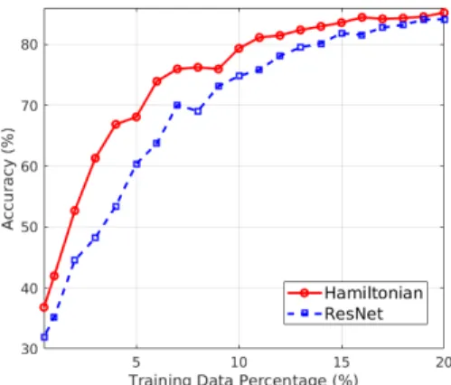
Figure 3: Hamiltonian vs ResNet test accuracy on CI- FAR10 with a small subset of training data.

in face of this data subsampling, instead of improving the state-of-the-art results. Therefore we intentionally use simple architectures: 4 blocks, each has 4 units, and the number of filters are16−64−128−256. For comparison, we use ResNet (He et al. 2016) as our baseline. CIFAR-10 has much more training data than STL-10 (50,000 vs 5,000), so we randomly subsample the training data from 20%to0.05%

for CIFAR-10, and from 80% to5% for STL-10. The test data set remains unchanged.

CIFAR-10 Fig. 3 shows the result on CIFAR-10 when decreasing the number examples in the training data from20%

to5%. Our Hamiltonian network performs consistently better in terms of accuracy than ResNet, achieving up to13%

higher accuracy when trained using just3%and4%of the original training data.

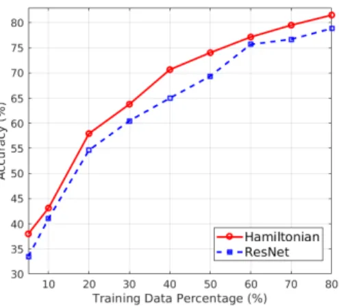
STL-10 From the result as shown in Fig. 4, we see that Hamiltonian consistently achieves better accuracy than ResNet with the average improvement being around3.4%.

(7)

Figure 4:Hamiltonian vs ResNet test accuracy for STL10 with a small subset of training data.

Especially when using just40%of the training data, Hamil- tonian has a5.7%higher accuracy compared to ResNet.

Training a 1202-layer Hamiltonian

To demonstrate the stability and memory-efficiency of the Hamiltonian network with arbitrary depth, we explore a 1202-layer architecture on CIFAR-10. An aggressively deep ResNet is also trained on CIFAR-10 in (He et al. 2016) with 1202 layers, which has an accuracy of92.07%. Our result is shown at the last row of Table 1. Compared with the original ResNet, our architecture uses only a half of parameters and obtains better accuracy. Since the Hamiltonian network is intrinsically stable, it is guaranteed that there is no issue of exploding or vanishing gradient. We can easily train an arbitrarily deep Hamiltonian network without any difficulty of optimization. The implementation of our reversible architecture is memory efficient, which enables a 1202 layer Hamil- tonian model running on a single GPU machine with 10GB GPU memory.

5 Conclusion

We present three stable and reversible architectures that connect the stable ODE with deep residual neural networks and yield well-posed learning problems. We exploit the intrinsic reversibility property to obtain a memory-efficient implementation, which does not need to store the activations at most of the hidden layers. Together with the stability of the forward propagation, this allows training deeper architectures with limited computational resources. We evaluate our methods on three publicly available datasets against several state-of-the-art methods. Our experimental results demonstrate the efficacy of our method with superior or on-par state-of-the-art performance. Moreover, with small amount of training data, our architectures achieve better accuracy compared with the widely used state-of-the-art ResNet. We attribute the robustness to small amount of training data to the intrinsic stability of our Hamiltonian neural network architecture.

6 Appendix

Proof: All eigenvalues of

J

in Eq.

(9)

are imaginary.

The Jacobian matrixJis defined in Eq. (9). IfAandBare two invertible matrices of the same size, thenABandBA have the same eigenvalues (Theorem 1.3.22 in (Horn and Johnson 2012)). If we define

J⁰= diag(σ⁰)

0 K₁ K2 0

K^T₁ 0 0 −K^T₂

= diag(σ⁰)

0 −K₁K^T₂ K2K^T₁ 0

:=DM, (23)

thenJandJ⁰ have the same eigenvalues.D is a diagonal matrix with non-negative elements, and M is a real anti- symmetric matrix such thatM^T = −M. Letλand v be a pair of eigenvalue and eigenvector ofJ⁰ =DM, then

DMv=λv, (24) Mv=λD⁻¹v, (25) v^∗Mv=λ(v^∗D⁻¹v), (26) whereD⁻¹ is the generalized inverse ofD. On one hand, sinceD⁻¹is non-negative definite,v^∗D⁻¹vis real. On the other hand,

(v^∗Mv)^∗=v^∗M^∗v=v^∗M^Tv=−v^∗Mv, (27) where∗represents conjugate transpose. Eq. 27 implies that v^∗Mvis imaginary. Therefore,λhas to be imaginary. As a result, all eigenvalues ofJare imaginary.

Implementation details

Our method is implemented using TensorFlow library (Abadi et al. 2016). The CIFAR-10/100 and STL-10 experiments are evaluated on a desktop with an Intel Quad-Core i5 CPU and a single Nvidia 1080 Ti GPU.

For CIFAR-10 and CIFAR-100 experiments, we use a fixed mini-batch size of 100 both for training and test data except Hamiltonian-1202, which uses a batch-size of 32.

The learning rate is initialized to be 0.1 and decayed by a factor of 10 at 80, 120 and 160 training epochs. The total training step is 80K. The weight decay constant is set to 2×10⁻⁴, weight smoothness decay is2×10⁻⁴ and the momentum is set to 0.9.

For STL-10 experiments, the mini-batch size is 128. The learning rate is initialized to be 0.1 and decayed by a factor of 10 at 60, 80 and 100 training epochs. The total training step is 20K. The weight decay constant is set to5×10⁻⁴, weight smoothness decay is3×10⁻⁴and the momentum is set to 0.9.

References

Abadi, M.; Agarwal, A.; Barham, P.; Brevdo, E.; Chen, Z.; Citro, C.; Corrado, G. S.; Davis, A.; Dean, J.; Devin, M.; et al. 2016.

Tensorflow: Large-scale machine learning on heterogeneous dis- tributed systems.arXiv preprint arXiv:1603.04467.

Arnold, V. I. 2012. Geometrical methods in the theory of ordinary differential equations. Springer Science & Business Media.

(8)

Arora, S.; Liang, Y.; and Ma, T. 2016. Why are deep nets reversible: A simple theory, with implications for training. ICLR- Workshop.

Ascher, U., and Petzold, L. 1998. Computer Methods for Ordi- nary Differential Equations and Differential-Algebraic Equations.

Philadelphia: SIAM.

Ascher, U. 2010.Numerical methods for Evolutionary Differential Equations. Philadelphia: SIAM.

Bellman, R. 1953. An introduction to the theory of dynamic pro- gramming. Technical report.

Bliss, G. A. 1919. The use of adjoint systems in the problem of differential corrections for trajectories.JUS Artillery51:296–311.

Bock, G. 1983. Recent advances in parameter identification techniques for ode. In Deuflhard, P., and Hairer, E., eds.,Numerical treatment of inverse problems. Boston: Birkhauser.

Cessac, B. 2010. A view of neural networks as dynamical systems.

International Journal of Bifurcation and Chaos.

Chang, B.; Meng, L.; Haber, E.; Tung, F.; and Begert, D. 2017.

Multi-level residual networks from dynamical systems view.arXiv preprint arXiv:1710.10348.

Cho, K.; Van Merri¨enboer, B.; Gulcehre, C.; Bahdanau, D.;

Bougares, F.; Schwenk, H.; and Bengio, Y. 2014. Learning phrase representations using rnn encoder-decoder for statistical machine translation.ACL.

Coates, A.; Ng, A.; and Lee, H. 2011. An analysis of single-layer networks in unsupervised feature learning. InAISTATS.

Coddington, E. A., and Levinson, N. 1955. Theory of ordinary differential equations. Tata McGraw-Hill Education.

Dinh, L.; Krueger, D.; and Bengio, Y. 2015. Nice: Non-linear independent components estimation.ICLR-Workshop.

Dinh, L.; Sohl-Dickstein, J.; and Bengio, S. 2016. Density estimation using real NVP.NIPS.

Dosovitskiy, A., and Brox, T. 2016. Inverting visual representations with convolutional networks. InCVPR.

Dundar, A.; Jin, J.; and Culurciello, E. 2015. Convolutional clustering for unsupervised learning.arXiv preprint arXiv:1511.06241.

E, W. 2017. A proposal on machine learning via dynamical systems.Communications in Mathematics and Statistics.

Esteva, A.; Kuprel, B.; Novoa, R. A.; Ko, J.; Swetter, S. M.; Blau, H. M.; and Thrun, S. 2017. Dermatologist-level classification of skin cancer with deep neural networks.Nature.

Gilbert, A. C.; Zhang, Y.; Lee, K.; Zhang, Y.; and Lee, H. 2017.

Towards understanding the invertibility of convolutional neural networks.arXiv preprint arXiv:1705.08664.

Gomez, A. N.; Ren, M.; Urtasun, R.; and Grosse, R. B. 2017.

The reversible residual network: Backpropagation without storing activations.NIPS.

Gunzburger, M. D. 2003. Perspectives in flow control and optimization. SIAM.

Haber, E., and Ruthotto, L. 2017. Stable architectures for deep neural networks.arXiv preprint arXiv:1705.03341.

Haber, E.; Ruthotto, L.; and Holtham, E. 2017. Learning across scales-a multiscale method for convolution neural networks.arXiv preprint arXiv:1703.02009.

He, K.; Zhang, X.; Ren, S.; and Sun, J. 2016. Deep residual learning for image recognition. InCVPR.

He, K.; Gkioxari, G.; Doll´ar, P.; and Girshick, R. 2017. Mask R-CNN. InICCV.

Horn, R. A., and Johnson, C. R. 2012.Matrix Analysis.

Hornik, K. 1991. Approximation capabilities of multilayer feed- forward networks.Neural networks.

Huang, G.; Sun, Y.; Liu, Z.; Sedra, D.; and Weinberger, K. Q. 2016.

Deep networks with stochastic depth. InECCV.

Huang, G.; Liu, Z.; Weinberger, K. Q.; and van der Maaten, L.

2017. Densely connected convolutional networks. CVPR.

Krizhevsky, A., and Hinton, G. 2009. Learning multiple layers of features from tiny images.

LeCun, Y.; Bengio, Y.; and Hinton, G. 2015. Deep learning. Na- ture.

Long, Z.; Lu, Y.; Ma, X.; and Dong, B. 2017. Pde-net: Learning pdes from data.arXiv preprint arXiv:1710.09668.

Lu, Y.; Zhong, A.; Li, Q.; and Dong, B. 2017. Beyond finite layer neural networks: Bridging deep architectures and numerical differential equations.arXiv preprint arXiv:1710.10121.

Lyapunov, A. M. 1992. The general problem of the stability of motion. International Journal of Control.

Mahendran, A., and Vedaldi, A. 2015. Understanding deep image representations by inverting them. InCVPR.

Nguyen, B. D., and McMechan, G. A. 2014. Five ways to avoid storing source wavefield snapshots in 2d elastic prestack reverse time migration.Geophysics.

Oord, A. v. d.; Dieleman, S.; Zen, H.; Simonyan, K.; Vinyals, O.;

Graves, A.; Kalchbrenner, N.; Senior, A.; and Kavukcuoglu, K.

2016. Wavenet: A generative model for raw audio. arXiv preprint arXiv:1609.03499.

Perez, E.; de Vries, H.; Strub, F.; Dumoulin, V.; and Courville, A. 2017. Learning visual reasoning without strong priors. arXiv preprint arXiv:1707.03017.

Pohlen, T.; Hermans, A.; Mathias, M.; and Leibe, B. 2017. Full resolution image compression with recurrent neural networks.CVPR.

Simmons, G. F. 2016.Differential equations with applications and historical notes. CRC Press.

Simonyan, K., and Zisserman, A. 2015. Very deep convolutional networks for large-scale image recognition.ICLR.

Ulbrich, S. 2002. A sensitivity and adjoint calculus for discontin- uous solutions of hyperbolic conservation laws with source terms.

SIAM J. Control and Optimization41:740–797.

Wu, Y.; Schuster, M.; Chen, Z.; Le, Q. V.; Norouzi, M.;

Macherey, W.; Krikun, M.; Cao, Y.; Gao, Q.; Macherey, K.; et al.

2016. Google’s neural machine translation system: Bridging the gap between human and machine translation. arXiv preprint arXiv:1609.08144.

Xie, S.; Girshick, R.; Doll´ar, P.; Tu, Z.; and He, K. 2017. Aggre- gated residual transformations for deep neural networks. CVPR.

Xiong, W.; Droppo, J.; Huang, X.; Seide, F.; Seltzer, M.; Stolcke, A.; Yu, D.; and Zweig, G. 2017. The microsoft 2016 conversational speech recognition system. InICASSP.

Yang, S.; Luo, P.; Loy, C. C.; Shum, K. W.; Tang, X.; et al. 2015.

Deep representation learning with target coding. InAAAI.

Zagoruyko, S., and Komodakis, N. 2016. Wide residual networks.

BMVC.

Zhang, C.; Bengio, S.; Hardt, M.; Recht, B.; and Vinyals, O. 2017.

Understanding deep learning requires rethinking generalization.

ICLR.

Zhao, J. J.; Mathieu, M.; Goroshin, R.; and LeCun, Y. 2016.ICLR- workshop.