Decision-making in complex and uncertain environments - Experimental studies in behavioral economics

Decision-making in complex and uncertain environments

-

Experimental studies in behavioral economics

Dissertation zur Erlangung des Grades eines Doktors der Wirtschaftswissenschaft

eingereicht an der Fakultät für Wirtschaftswissenschaften der Universität Regensburg

vorgelegt von: Johannes Moser

Berichterstatter: Prof. Dr. Andreas Roider und Prof. Jörg Oechssler, Ph.D.

Tag der Disputation: 22. November 2019

Universit¨ at Regensburg

Dissertation

Decision-making in complex and uncertain environments

Experimental studies in behavioral - economics

Inauguraldissertation

zur Erlangung des akademischen Grades eines Doktors der Wirtschaftswissenschaften

der Universit¨at Regensburg

Erstbetreuer: Prof. Dr. Andreas Roider Zweitbetreuer: Prof. J¨org Oechssler, Ph.D.

Vorgelegt im Juli 2019 von:

Johannes Moser

Acknowledgments

First of all, I want to thank my first supervisor Andreas Roider for his guidance and support during the work on my thesis. I always had the opportunity to talk to him about my research and I greatly benefited from his vast experience. Additionally, he also assisted me in a lot of organizational matters, such as applying for conferences or during the revision of a paper. Overall, Andreas always expected a high level of motivation and performance from me, but at the same time he made sure that I could fully concentrate on my research. This made it possible for me to write this thesis in its present form.

I further want to thank my colleagues from the University of Regensburg and my fellow students from the International Graduate Program “Evidence-Eased Eco- nomics” (EBE). In internal presentations as well as in discussions with my peers, I received great feedback and comments which helped me to further improve my own work. Also the atmosphere within this group was always very pleasant.

At this point, I also want to emphasize how much I profited from my membership in the International Graduate Program “Evidence-Based Economics” (EBE) of the Elite Network of Bavaria. The course program of the EBE was structured in a very sensible way and it was very much in line with my own research interests. Through the EBE I got in touch with a lot of interesting people and experts from all over the world. Additionally, I received a generous funding which made it possible for me to attend several national and international conferences, where I got the opportunity to present my own research. Furthermore, because of the funding, I was able to conduct the experiments which I used for my thesis.

Looking back, I can say that working on my thesis was a demanding, but re- warding journey. This thesis is the result of four interesting years of research in the field of behavioral and experimental economics and I hope that this work will give the reader a good insight into this field.

Johannes Moser, July 2019

F¨ ur meine Eltern

Contents

1 Introduction

1

2 Hypothetical thinking and the winner’s curse

5

2.1 Literature review . . . . 9

2.2 The model . . . 12

2.3 Experimental design . . . 14

2.3.1 Implementation . . . 14

2.3.2 Basic setup . . . 15

2.3.3 Treatments . . . 16

2.3.4 Behavioral predictions . . . 17

2.4 Results . . . 19

2.4.1 Overall bidding pattern in stage I . . . 19

2.4.2 Bidding behavior in stage II . . . 20

2.4.3 Profits . . . 24

2.4.4 Differentiation between low and high signals . . . 27

2.4.5 Cursed equilibrium . . . 29

2.4.6 Analysis on subject level . . . 30

2.5 Discussion . . . 32

3 Correlation neglect and voting

34 3.1 Experimental design . . . 36

3.1.1 General setting . . . 36

3.1.2 Part 1 . . . 37

3.1.3 Part 2 (Treatments) . . . 38

3.1.4 Post-experimental questionnaire . . . 38

3.1.5 Implementation . . . 39

3.2 Properties of the game . . . 40

3.3 Results . . . 42

3.4 Discussion . . . 46

4 Leadership in dynamic public goods games

48 4.1 Literature review . . . 49

4.2 Experimental design and procedures . . . 51

4.2.1 Part I . . . 51

4.2.2 Part II . . . 52

4.2.3 Participants and procedures . . . 54

4.3 Hypotheses and research questions . . . 54

4.3.1 Wealth . . . 54

4.3.2 Inequality . . . 56

4.3.3 Leader types . . . 56

4.4 Results . . . 57

4.4.1 Wealth . . . 58

4.4.2 Inequality . . . 59

4.4.3 Payoff dominance accross rounds . . . 62

4.4.4 Further analysis of the

LEAD

treatment . . . 63

4.5 Discussion . . . 69

5 Consistency of cooperation types

71 5.1 Design and procedures . . . 71

5.1.1 Protocol . . . 71

5.1.2 Sequential Prisoner’s Dilemma (SPD) . . . 72

5.1.3 Sequential Public Goods Game (FGF) . . . 73

5.2 Results . . . 74

5.2.1 Contribution paths in

FGF

by

SPD

type . . . 74

5.2.2 Relationship between classification methods . . . 75

5.3 Summary and discussion . . . 79

6 Conclusion

80

A Figures & Tables (Section 2 - winner’s curse)

89

B Proofs (Section 2 - winner’s curse)

95

C Instructions (Section 2 - winner’s curse)

97

D Control questions (Section 2 - winner’s curse)

103

E Proofs (Section 3 - correlation neglect)

104

F Instructions (Section 3 - correlation neglect)

107

G Voting screens (Section 3 - correlation neglect)

110

H Balancing table (Section 4 - leadership)

111

I Translated instructions (Section 4 - leadership)

112

J Instructions (Section 5 - cooperation types)

116

List of Figures

2.1 Illustration of the treatments . . . 17

2.2 Median and mean bids in stage I . . . 20

2.3 Range of unsophisticated and sophisticated bids . . . 21

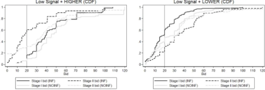
2.4 Cumulative distribution functions - Low signals . . . 22

2.5 Cumulative distribution functions - High signals . . . 22

2.6 Changing of bids in stage II (treatment INF) . . . 28

2.7 Changing of bids across the rounds . . . 29

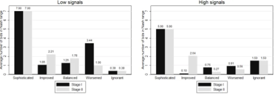
2.8 Bids in Nash range by bidder type . . . 31

3.1 Preferences across treatments . . . 43

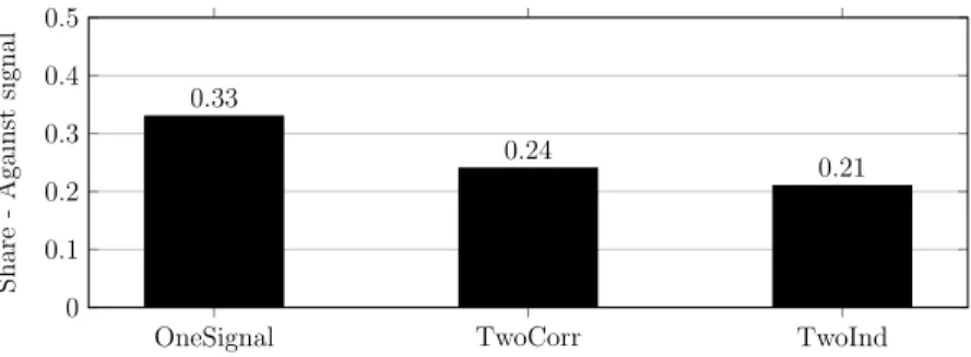
3.2 Voted against signal when signal is different to preference . . . 43

3.3 Votes by treatment when signal is different to preference . . . 44

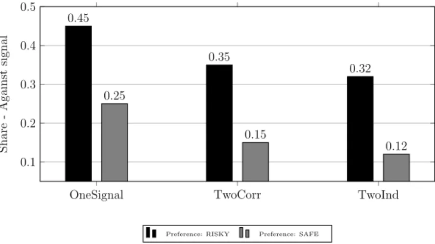
3.4 Votes by preference when signals are mixed . . . 46

4.1 Payoff structure of the sequential prisoner’s dilemma . . . 51

4.2 Average endowment at the end of each round . . . 58

4.3 Average Gini coefficient at the end of each round by treatment . . . . 60

4.4 First emergence of no PAYOFF DOMINANCE . . . 62

4.5 Leader’s relative contribution by behavioral type and round . . . 65

4.6 Relationship between leader’s first contribution and final endowment 67 4.7 Average endowment by treatment + leader/non-leader . . . 68

4.8 Bad leadership . . . 68

4.9 Good leadership . . . 69

5.1 Payoff structure of the sequential prisoner’s dilemma . . . 72

5.2 Contribution paths by

SPD

classification in

FGF

. . . 74

5.3 Venn diagrams of SPD and FGF-T (Th¨oni and Volk, 2018) . . . 78

5.4 Venn diagrams of SPD and FGF-F (Fallucchi et al., 2018) . . . 79

A.1 Typical decision screen in stage I. . . . 89

A.2 Typical decision screen in stage II (treatment INF). . . . 90

A.3 Typical decision screen in stage II (treatment NOINF). . . . 91

A.4 Distribution of bids in stage I . . . 92

A.5 Distribution of bids in stage II (INF) . . . 92

A.6 Distribution of bids in stage II (NOINF) . . . 92

A.7 Corridor of Nash range . . . 93

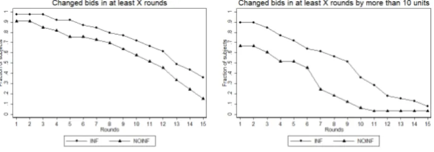
A.8 Fraction of changed bids across the 15 rounds . . . 94

G.1 Typical voting screen in treatment

OneSignal

. . . 110

G.2 Typical voting screen in treatment

TwoCorr

. . . 110

G.3 Typical voting screen in treatment

TwoInd

. . . 110

List of Tables

2.1 Prediction of other player’s signal for different constellations . . . 18

2.2 Winner’s curse and loser’s curse in Stage I for different constellations of signals. Winner’s curse: won, but with a negative payoff. Loser’s curse: lost, but could have won the auction with a positive payoff. . . 20

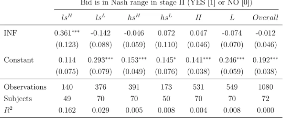
2.3 Regression Table - Bid in Nash range (Stage II) . . . 23

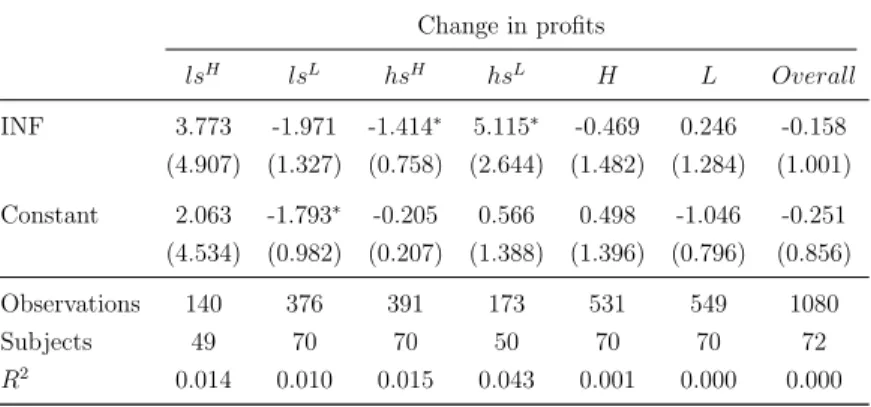
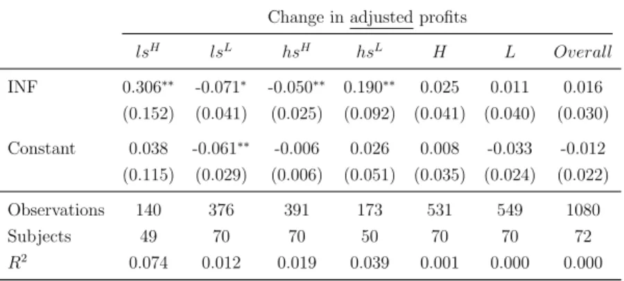
2.4 Regression Table - Change in profits . . . 25

2.5 Regression Table - Change in adjusted profits . . . 26

2.6 Number of different bidding types across treatments . . . 31

3.1 Payoff structure in part 1 . . . 37

3.2 Payoff structure in part 2 . . . 39

3.3 Self-reported risk preferences . . . 45

4.1 Cooperation types . . . 52

4.2 Structure of periods and rounds . . . 52

4.3 Regression Table - Final endowment . . . 59

4.4 Regression Table - GINI coefficient . . . 61

4.5 Regression Table - Violation of payoff dominance . . . 63

4.6 Regression Table - Matching of leader contribution (absolute and rel- ative) . . . 64

4.7 Regression Table - Final endowment (only

LEAD)

. . . 66

5.1 Cooperation types in

SPD

. . . 73

5.2 Regression Table - Contribution paths . . . 75

5.3 Cooperation types in Th¨oni and Volk (2018) . . . 76

5.4 Types in

SPD

and

FGF

(Refinement of Th¨oni and Volk, 2018) . . . . 76

5.5 Cooperation types in Fallucchi et al. (2018) . . . 77

5.6 Types in

SPD

and

FGF

(Refinement of Fallucchi et al., 2018) . . . . 77

A.1 Regression Table - Bid in Nash range (Stage I) . . . 93

A.2 Regression Table - Changes across the bidding ranges . . . 94

E.1 Combinations of signals . . . 104

H.1 Number of different cooperation types across treatments . . . 111

1 Introduction

Behind all things are reasons. Reasons can even explain the absurd. Do we have the time to learn the reasons behind the human being’s varied behavior? I think not. Some take the time.

– Log Lady, Twin Peaks

There is a large body of empirical evidence that people do not always behave accord- ing to game theoretic predictions in many economic or social environments. Possible deviations from standard-economic behavior can occur when individuals have either (i) non-standard beliefs, which are systematically biased, (ii) non-standard prefer- ences, such as preferences for fairness, or (iii) when they engage in imperfect utility maximization, for example, because of limited attention and only consider salient alternatives in their choice sets (Rabin, 2002). This thesis addresses issues related to such forms of boundedly rational behavior and non-standard utility maximization.

As a general term, for all deviations from standard-economic behavior mentioned above, I will use the expression “non-standard decision-making” in this thesis.

The field of behavioral economics deals with questions concerning non-standard decision-making, by combining elements from economics and psychology. This area of economic research has become increasingly important in recent years, which was also reflected in the Nobel Prize for Richard H. Thaler in 2017. Research in this field has been able to explain many empirical findings and economic puzzles, such as charitable giving (Ariely, Bracha, and Meier, 2009), blood donations (Mellstr¨om and Johannesson, 2008), overbidding in auctions (Crawford and Iriberri, 2007), or default effects in retirement savings (Madrian and Shea, 2001).

With my own work, I want to contribute to the vast experimental literature in behavioral economics. For this purpose, I will look at three different environments in which non-standard decision-making is commonly observed: common value auctions, public good games, and elections. The main aims of my research in these areas are the following: (i) finding the underlying channels of non-standard decision- making; (ii) investigating how the occurrence of potential cognitive mistakes can be reduced; (iii) checking whether mental shortcuts, or heuristics, are always irrational or whether they can be sometimes beneficial for individuals or groups and even lead to more socially efficient outcomes; (iv) furthermore, I am interested in the reasons and the economic consequences of cooperative and non-cooperative behavior.

With this, I would like to answer questions that have not yet been conclusively

clarified in the literature so far. My empirical research strategy relies on laboratory

and online experiments. The thesis will consist of four main chapters (Sections 2,

3, 4, and 5) following after the introduction.

The first chapter (Section 2) investigates the relationship between the winner’s curse and mistakes in hypothetical thinking in the context of common value auc- tions.

¹

There is evidence that bidders fall prey to the winner’s curse because they fail to extract information from hypothetical events - like winning an auction. In this chapter, I investigate experimentally whether bidders in a common value auc- tion perform better when the requirements for this cognitive issue - also denoted by contingent reasoning - are relaxed, leaving all other parameters unchanged. For my underlying research question, I used a lab experiment with two stages. In stage I, the subjects participate in a non-standard common value auction, called the wallet game, in which a na¨ıve bidding strategy can lead to both winner’s curse and loser’s curse. In stage II, the subjects in the treatment group learn whether their initial bid was the winning bid or not and they get the opportunity to change this bid.

In this sense, the bidders face the same decision problems as in stage I again, but the need for hypothetical thinking is reduced in stage II. More generally, I want to answer the question whether models focusing on inconsistent beliefs of individuals, like cursed equilibrium and level-k (Eyster and Rabin, 2005; Crawford and Iriberri, 2007) or approaches concerning contingent reasoning on hypothetical future events (Charness and Levin, 2009; Ivanov, Levin, and Niederle, 2010; Esponda and Vespa, 2014) are more suitable for explaining the winner’s curse.

In summary, the main questions I want to answer in this chapter are:

1. Do subjects in a common value auction perform better when they already learn ex ante, before the final payoffs are known, whether their bid is the winning bid or not?

2. Are approaches concerning mistakes in contingent reasoning or belief-based models like cursed equilibrium more accurate to explain the winner’s curse?

The second chapter (Section 3) deals with another cognitive mistakes known as correlation neglect.

²

This bias refers to underestimating the degree to which various sources of information may be correlated. Typical examples for this issue are the news media or markets for financial assets. In an online experiment, I tested how the presence of correlation neglect affects the outcome in a collective voting problem. My work aims to supplement the existing experimental literature on correlation neglect by implementing a theoretical work of Levy and Razin (2015a).

The experimental setup I used, provides an environment that includes the main features of their theoretical model: subjects with ideological preferences who receive an imperfect signal about the state of the world - which might differ from their

1This chapter is based onMoser(2019).

Available under:https://doi.org/10.1007/s11238-019-09693-9

2This chapter is based onMoser and Wallmeier(2019).

preferences - and a collective decision via majority vote. So the participants in my experiment are confronted with two conflicting objectives which they have to include in their maximization problem. Since political preferences are difficult to measure accurately, I focused on an approach where the choice of two alternatives depended on the risk preferences of the participants. On the one hand this makes the whole task more abstract, but on the other hand clear statements can be made about the effect of correlation neglect, when subjects are affected by personal preferences. To measure the effect of correlation neglect, the participants either received one signal, two perfectly correlated signals, or two independent signals about a state of the world in a between-subject design.

In summary, the main questions I want to answer in this chapter are:

1. Are subjects prone to correlation neglect in a collective decision problem - even though the correlation of information is presented in an obvious way?

2. What is the effect of correlation neglect on the outcome of an election where voters are influenced by ideological preferences?

The third chapter (Section 4) presents an experiment, where I tested whether leadership can influence the contribution pattern of individuals in a public goods game with growth.

³

In this chapter, I combine existing experiments concerning (i) leadership in static public goods games (see, for example, Moxnes and Van der Heijden, 2003; G¨ uth, Levati, Sutter, and Van Der Heijden, 2007) and (ii) experiments on dynamic public goods games with growth (see, for example, G¨achter, Mengel, Tsakas, and Vostroknutov, 2017). In my setup, leadership is associated with role model behavior or leading-by-example. This means that the leader has no formal power, but simply acts as first-mover. Through the dynamic setting, where growth is possible, I can investigate the long run effect of leadership. Additionally, I check whether the behavioral type of the leader has an effect on the success of the group.

To determine the cooperation type of each individual, I used a sequential prisoner’s dilemma where the participants had to make their decisions via strategy method.

In summary, the main questions I want to answer in this chapter are:

1. Does leading-by-example yield an improvement in a dynamic setting with en- dowment carryover?

2. Does the behavioral type of the leader affect the group’s performance?

The fourth chapter (Section 5) thematically ties in with the third chapter.

⁴

While, I show in the third chapter that cooperation types have a high predictive

3This chapter is based onEichenseer and Moser(2019b).

4The fourth chapter is based onEichenseer and Moser(2019a).

power concerning the success of a group, I demonstrate in the fourth chapter that dif- ferent methods for eliciting cooperation types are consistent to a large extent. More preciously, I compare a one-shot public goods game with strategy method, using the procedure of Fischbacher, G¨achter, and Fehr (2001), with a sequential prisoner’s dilemma, which was for example used in Miettinen, Kosfeld, Fehr, and Weibull (2017) and Kosfeld (2019). Furthermore, I want to investigate which method yields more valid results depending on the underlying research question.

In summary, the main questions I want to answer in this chapter are:

1. Are two structurally different methods for classifying cooperation types con- sistent?

2. Which of these methods yields the more valid results?

This thesis concludes with a final review of the conducted experiments, where I summarize the most important results and findings of my work (Section 6).

To answer the underlying questions, I made use of economic experiments, either in the laboratory or as online experiments. Controlled lab and online experiments have a few important advantages compared to field experiments or observational data. For example, (i) subjects can be randomly assigned to different treatment groups to rule out any selection biases and (ii) the researchers can keep specific variables constant in the lab, which is not always possible in the field. This makes it easier to make causal inferences. The lab experiments for the first and third chapter were programmed in zTree (Fischbacher, 2007) and conducted in the Regensburg Economic Science Lab (RESL). The online experiment for the second chapter was programmed in LimeSurvey and conducted on the research platform Prolific. The online experiment for the fourth chapter was programmed in LimeSurvey and con- ducted on Amazon Mechanical Turk (MTurk). For the experiments, I received a generous funding through the International Doctoral Program “Evidence-Based Economics” of the Elite Network of Bavaria.

Overall, I hope that my thesis can contribute to the vast literature on non-

standard decision-making in behavioral economics by providing some new ideas and

motivations which hopefully might further help to identify potential cognitive mis-

takes and ultimately help to avoid irrational behavioral patterns.

2 Hypothetical thinking and the winner’s curse ⁵

The winner’s curse is a well-known empirical phenomenon in common value auc- tions, which was first described by Capen, Clapp, and Campbell (1971). They showed that many oil companies in the 1960’s and 1970’s had to report a drop in profit rates because of systematic overbidding in auctions for drilling rights. Later experimental evidence for the winner’s curse was also found in a large number of lab studies (see, for example, Bazerman and Samuelson, 1983; Thaler, 1988; Charness and Levin, 2009; Ivanov, Levin, and Niederle, 2010).

I show in an experimental setup that bidders are more likely to avoid the win- ner’s curse when they are informed, before submitting a bid, whether their bid is the winning bid or not. By giving the subjects this information, I weaken the require- ment for them to condition their bid on winning the auction: winning or losing are now not hypothetical anymore, and the adverse selection issue of winning an auction with a common value for all bidders becomes more salient. The findings of my thesis suggest that mistakes in hypothetical thinking seem to explain a substantial part of the winner’s curse. Thus, approaches that focus on this mental process might be more suitable for explaining this phenomenon than belief-based models like cursed equilibrium (Eyster and Rabin, 2005), which state that the winner’s curse is mainly driven by inconsistent beliefs. Herewith, this thesis attempts to shed light on the ongoing debate on whether models, focusing on the erroneous belief formation of individuals, like cursed equilibrium and level-k (Eyster and Rabin, 2005; Crawford and Iriberri, 2007)

⁶

or approaches concerning contingent reasoning on hypothetical future events (Charness and Levin, 2009; Ivanov, Levin, and Niederle, 2010; Esponda and Vespa, 2014) are more suitable for explaining the winner’s curse.

Contingent reasoning refers to the ability of thinking through hypothetical sce- narios and to perform state-by-state reasoning. There is evidence that people have difficulties engaging in this cognitive task. While this is well documented in the psychological literature (see, for example, Evans, 2007; Nickerson, 2015; Singmann, Klauer, and Beller, 2016), economists devoted little attention to this issue for a long time. However, in the more recent economic literature this topic appears more and more frequently (see, for example, Charness and Levin, 2009; Louis, 2013; Esponda and Vespa, 2014; Ngangou´e and Weizs¨acker, 2015; Levin, Peck, and Ivanov, 2016;

5This chapter is a slightly modified version ofMoser(2019).

6Both models fall into the category of belief-based models, since the cause manifesting in the winner’s curse is seen in the belief formation of individuals. The general assumptions of Bayesian Nash Equilibrium are still fulfilled, in the sense that subjects best-respond to beliefs, but the as- sumption about the consistency of beliefs is relaxed. In cursed equilibrium, the degree ofcursedness is given byχ∈[0,1], i.e., the belief that with some probabilityχthe actions of the opponents do not depend on their types. A value of 0 is equivalent to the usual Bayesian Nash Equilibrium, whereas a value of 1 corresponds to a setting in which the players do not assume any correlation between the actions of a player and his type, which is also denoted asfullycursed equilibrium.

Esponda and Vespa, 2016; Li, 2017; Koch and Penczynski, 2018).

In contrast to belief-based models, like cursed equilibrium, the concept of con- tingent reasoning has still received very little formal treatment. Li (2017) represents the first attempt to capture this mental process formally by introducing the concept of obviously strategy-proof (OSP) mechanisms.

⁷

A major contribution of Li’s paper is to explain why subjects perform better in ascending bid auctions compared to sealed bid auctions. However, it cannot explain why common value auctions might be more challenging for the bidders than private value auctions. For this reason, the concept of OSP mechanisms is not sufficient to fully capture the most relevant aspects of the winner’s curse.

Can a broader definition of contingent reasoning explain why bidders fall prey to the winner’s curse? To answer this question I will go back one step from OSP mechanisms and focus only on the events of winning or losing an auction - which provide information about the true value of a good in common but not in private value auctions. Bidders in common value auctions now face two cognitive hurdles.

First, they have to be able to recognize and identify several hypothetical scenarios which might possibly occur (e.g., winning or losing an auction) and second, the bidders have to be able to infer information from such hypothetical events. The question is which of these cognitive tasks is more challenging for subjects and to what extent they affect the likelihood of the winner’s curse to occur. There are three possibilities: (i) bidders are perfectly able to perform state-by-state reasoning, but they neglect the informational content of the other bidders’ actions and, hence, the informational content of winning an auction as proposed by cursed equilibrium; (ii) bidders take into account that the bids of the other players are correlated with their signals, but they are not able to identify the relevant states to condition on in the first place; (iii) bidders are neither able to perform state-by-state reasoning, nor do they take into account the informational content of winning an auction.

In this chapter, I test experimentally whether subjects in an auction are able to infer information from the events of winning or losing if these are not hypothetical anymore. For this purpose, I constructed a second-price auction in which the bidders learn whether a bid, which was considered optimal ex ante, is the winning bid or not (but without learning their payoff yet) and they receive the possibility to change this bid. This treatment intervention is similar to the sequential treatment in Esponda and Vespa (2014) where participants in an election learned whether their votes were

7According toLi(2017), a mechanism is OSP if and only if an optimal strategy can be found without the necessity of performing contingent reasoning. However, Li’s definition of contingent reasoning is very strict in a game-theoretic sense as it does not only involve conditioning on different broader states of the world or future events (such as conditioning on being the winner in an auction or conditioning on being the pivotal voter in an election), but also conditioning on each possible decision node in a given information set. Additionally, there is only a differentiation between whether a game is OSP or not, but no distinction between “more” or “less” contingent reasoning.

pivotal or not before they had to cast a vote. In contrast to Koch and Penczynski (2018) my approach is weaker, since it does not remove the need for contingent reasoning at all, but only partly in a specific context. However, thereby I am able to show whether such a weak manipulation, on a feedback basis, is sufficient for subjects to improve their bids, without changing the whole structure of the game.

Additionally, it has to be noted that even Koch and Penczynski (2018) did not meet the strict requirements of completely eliminating the necessity for contingent reasoning, according to the definition of Li (2017). This further emphasizes the urgent need for a consistent definition of this term.

The auction model I used in the experiment is based on a second-price sealed bid auction similar to the wallet game proposed by Klemperer (1998) and the model used in Avery and Kagel (1997), which is a non-standard common value auction.

The basic idea of the game is the following: two players, indexed by

i

= 1, 2, receive a private

iid

signal,

xi

, drawn from some commonly known distribution. In a second- price sealed bid auction they bid for an object worth

v

=

x1

+

x2

. This game is played in two stages. In stage I, the subjects participate in the wallet game against a random opponent. In stage II, the subjects play the same auctions again, against the decisions of the former opponent, but this time the subjects in the treatment group are informed whether their initial bid was the winning bid or not. In this sense, the bidders receive information about some realized event before they have to come up with a bid.

⁸

Apart from knowing whether their bid is the winning or losing bid, the subjects face exactly the same decision problem as in stage I.

My design allows a clear distinction between mistakes in contingent reasoning and cursed equilibrium since two crucial assumptions of the latter are that (i) no (or only a partial) correlation between the other players’ actions and types is assumed and (ii) bidders still best-respond given their beliefs. Hence, for a “cursed” bidder the information on whether his bid is higher or lower than the bid of the opponent, does not provide him further information which would be relevant for updating his bid. For fully cursed bidders this argument is straightforward, but it also holds for partly cursed bidders because of the best-response assumption. By definition, the bid of a cursed bidder is already evaluated conditional on winning in stage I, albeit a partly cursed bidder implicitly assumes that winning is less informative than in equilibrium. This means, the feedback of winning in stage II provides no further relevant information, since it is already included in the decision of a partly cursed bidder in stage I.

The reason for choosing the wallet game, instead of a more standard model for common value auctions, is that in this game a na¨ıve bidding strategy can lead to both

8See alsoEsponda and Vespa(2016) for a distinction between static and dynamic choice situa- tions.

over- and underbidding, relative to the symmetric equilibrium strategy, depending on whether the private signal is low or high. In this sense, there can be both a winner’s and a loser’s curse (see also Holt and Sherman, 1994).

⁹

This property is useful for two reasons. First, I am able to control for psychological explanations, stating that the winner’s curse is mainly driven by emotional factors of winning (see, for example, Van den Bos, Li, Lau, Maskin, Cohen, Montague, and McClure, 2008;

Astor, Adam, J¨ahnig, and Seifert, 2013). Second, and more importantly, I am able to check whether bid shading in stage II is due to proper Bayesian updating or just a rule of thumb when learning that a certain bid was the winning bid. In my setup, bid shading is only advisable for low signals, but not for high signals. Thus, the subjects have to differentiate between these two kinds of signals, instead of following the simple decision rule “decrease your bid, when you learn that your bid was the winning bid”.

The findings of my thesis reveal two important observations:

(i) Bidders are more likely to avoid the winner’s curse and the loser’s curse in stage II when they are informed whether their bid is the winning bid or not, given that the respective information has a sufficiently high predictive power concerning the opponent’s signal. This suggests that the crucial cognitive hurdle for bidders in a common value auction is not forming beliefs about the opponents’ behavior, but identifying the relevant states to condition on in the first place.

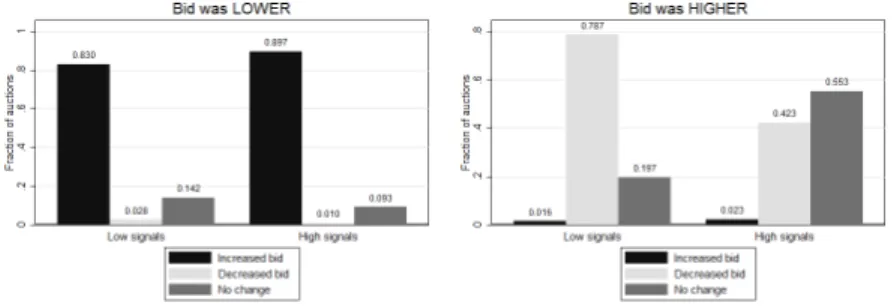
(ii) Information can also be negative for the bidders, depending on the context.

The subjects in my experiment differentiated only imperfectly between situations in which decreasing (increasing) a bid is rational and those in which it is not and they often used simple heuristics instead of making strategic changes. This behavior might be partly explained by an actual joy of winning or, to be more precise, a disappointment of losing. When subjects learned that they lost an auction in stage I, most of them increased their bid in stage II, regardless of having a low or high private signal. Conversely, when subjects learned that they won an auction in stage I, they acted more strategically and bids for low signals were decreased at a much higher rate compared to bids for high signals (78.7% vs. 42.3%).

This chapter is organized as follows. Section 2.1 will provide an overview about the current literature closely related to my research topic. Section 2.2 will present the underlying theoretical model for the experiment. Section 2.3 describes the ex- perimental design. Section 2.4 presents and discusses the results of the experiment.

Section 2.5 concludes the chapter.

9A loser’s curse can be understood as losing an auction, but the bidder could have won with a positive payoff.

2.1 Literature review

This thesis is the first to investigate the direct effect of the information of winning (or losing) in the context of a common value auction. The novelty of my design is that I use a dynamic choice setting `a la Esponda and Vespa (2014) in a sealed bid auction. Similar to them, I want to differentiate between mistakes in hypotheti- cal thinking and problems with extracting information from the opponents’ actions.

With this setup I am able to test whether potential errors in common value auctions occur due to an inability of performing contingent reasoning or due to inconsistent beliefs as proposed by cursed equilibrium. To the best of my knowledge, none of the recent approaches provided a similar framework. For example, the experiment by Charness and Levin (2009) is a single decision maker problem in an adverse selection environment. Additionally, they measured the effect of contingent reasoning only indirectly by transforming their initial game into a set of simple lotteries. Ivanov, Levin, and Niederle (2010) showed that belief-based models, like cursed equilibrium, might be not that powerful in explaining the winner’s curse, but they provided no alternative explanation. The paper of Koch and Penczynski (2018) is also closely re- lated to my work. So far they are the only ones who combined contingent reasoning and belief-based models in their experiment. However, they focused on a different aspect of contingent reasoning, not directly related to the event of winning an auc- tion. Finally, Levin, Peck, and Ivanov (2016) used Dutch auctions and showed that in this format conditioning on winning is more salient compared to a strategically equivalent first-price auction. All of these papers will be discussed in more detail in the following part.

As explained above, the paper most closely related to my own work is the one by Esponda and Vespa (2014). They created a common value voting experiment where a subject interacted with two computers. The main task for the subject was to submit a vote for a ball which was either red or blue. Due to the commonly known voting algorithm of the computers, the vote of the subject was only relevant when the ball was blue and, hence, the optimal choice for the subject was always to vote for blue. Esponda and Vespa (2014) observed that subjects made significantly less errors in a sequential election, where the voters knew whether they were pivotal or not, compared to a simultaneous election, where the voters were not informed about their pivotality. Similarly, in their lab experiment Ngangou´e and Weizs¨acker (2015) found that traders in a financial market setting performed better in a sequential trading mechanism where no Bayesian updating on hypothetical events was required.

Charness and Levin (2009) conducted an experiment constructed as a simple

individual choice problem similar to an acquiring a company game, which is based

on a lemon market (Akerlof, 1970), to investigate the driving mechanisms behind

the winner’s curse. The results of their paper revealed that most of the subjects sys- tematically overbid even though the strategy of the computerized seller was known and, hence, there was no need for the subjects to form beliefs about his behav- ior. This pattern was reduced in a setting where the bidding task was transformed into a set of simple lotteries with no requirement of thinking in hypothetical situa- tions. However, transforming the initial game into a simple lottery task changes the whole structure of the game and so it remains difficult to extract a causal effect of hypothetical thinking.

Ivanov, Levin, and Niederle (2010) used a similar approach as Charness and Levin (2009), but they conducted their experiment in an actual auction context us- ing the maximal game.

¹⁰

The aim of their experiment was not to look at the effect of contingent reasoning, but rather to disprove that the winner’s curse is driven by inconsistent beliefs. Ivanov, Levin, and Niederle (2010) observed significant over- bidding which was not reduced in a modified setting of the maximal game where the beliefs of the participants were explicitly formed and, thus, belief-based models, like cursed equilibrium, had little explanatory power. However, Costa-Gomes and Shimoji (2015) criticized Ivanov, Levin, and Niederle (2010) for the misuse of some of the game theoretical concepts, arguing that some of their findings can indeed be explained by belief-based models. Similarly, Camerer, Nunnari, and Palfrey (2016) argued that the observed behavior of the subjects in Ivanov, Levin, and Niederle (2010) can be explained by belief-based models if they are combined with a quantal response model. Under this extension the assumption of perfect best-reply behavior in cursed equilibrium and level-k model is relaxed and stochastic choices are allowed.

They showed that this extended model fits very well to the data of Ivanov, Levin, and Niederle (2010).

¹¹

My approach is different from the one in Ivanov, Levin, and Niederle (2010).

Rather than showing that bidders do not best-respond, even though their beliefs are explicitly formed, I show that bidders in my setup react to information which is, by definition, not relevant for the updating process of a “cursed” bidder.

¹²

Koch and Penczynski (2018) conducted an auction game similar to the one in

10Ivanov, Levin, and Niederle(2010) criticized that the acquiring a company game, used in Charness and Levin(2009), represents a lemon market and not a common value auction. Thus, it seems problematic to extend the findings from their experiment to common value auctions in general. They also claimed that it can make a difference whether a subject plays against other people or against a computer. In fact,Ivanov, Levin, and Niederle(2010) also used a computer treatment, but in their case the computer mimicked the subject’s own past strategy.

11However,Camerer, Nunnari, and Palfrey(2016) also assume that, if theperfectbest-reply assumption of cursed equilibrium and level-kmodel is maintained, these models are very bad in predicting the behavior in maximal value games.

12In the setup ofIvanov, Levin, and Niederle(2010) one could still argue that the belief formation of a cursed bidder takes place in an isolated “black box” and is not affected by information about the opponent’s behavior which is given to such a bidder. This is not an issue in my design.

Kagel and Levin (1986) to investigate how explanations concerning contingent rea- soning and belief-based models interact. The authors found that the relaxation of both cognitive requirements had a significant effect on avoiding the winner’s curse.

To identify the effect of contingent reasoning on the bidding behavior of the subjects, the authors used a transformed version of the original game, where both bidders re- ceived the same information about an object with a stochastic value, instead of different private signals. In this sense, there was no need for the bidders to con- dition on whether their own signal was relatively low or high. This is different from my approach, where I focus on the direct effect of the information of winning an auction. Additionally, I only changed one parameter in stage II, whereas Koch and Penczynski (2018) used two different games, but with the same best-response functions and equilibria.

Levin, Peck, and Ivanov (2016) used an experiment to investigate the impact of Bayesian updating and non-probabilistic reasoning (referred to as contingent reason- ing in this thesis) on avoiding the winner’s curse. They used common value Dutch and common value first-price auctions based on the model in Kagel, Harstad, and Levin (1987) and compared both versions to quantify the effect of non-probabilistic reasoning. Additionally, they measured the skills of the participants in Bayesian updating and non-probabilistic reasoning through a questionnaire, which the sub- jects had to answer before they participated in the auctions, and showed that both cognitive skills had a significant effect on avoiding the winner’s curse, resulting in higher earnings for the subjects. The authors also showed that subjects performed better in a Dutch auction, where the auction ended when the first subject stopped the clock, compared to a Dutch auction, where the auction ended when the last subject stopped the clock and no subject received any feedback about whether he is the highest bidder. In the first setting, a bidder knows, in the moment of stopping the clock, that he is the highest bidder and, hence, it is more salient for him to con- dition his bid on winning compared to the second setting with a “silent” clock. The authors concluded that bidders can better handle the winner’s curse if the require- ments for this form of hypothetical thinking are reduced.

¹³

Note that this form of a Dutch auction is not comparable to the sequential approach of Esponda and Vespa (2014) because, strictly speaking, only after stopping the clock the subject learns that he is the highest bidder.

¹⁴

The advantage of my design is that the bidders in stage II receive this information before they have to come up with a bid.

13As a further robustness check, the authors also used private-value auctions, where they did not find a significant difference between these two kinds of Dutch auctions.

14A further problem of Dutch auctions is that the bidders have to make a decision pressed for time. This can lead to various effects on emotional level (see, for example,Adam, Kr¨amer, and Weinhardt,2012;Adam, Kr¨amer, and M¨uller,2015).

2.2 The model

In the following section I present a formal description of the auction game used in the experiment. This game is based on the wallet game proposed by Klemperer (1998) and the model used in Avery and Kagel (1997). Henceforth, this game will be denoted as the wallet game, although it is slightly different from the original one.

¹⁵

There are two players, indexed by

i

= 1, 2. Each player

i

receives a signal

xi

from the set

X

=

{0,

1, . . . ,9, 10, 50, 51, . . . , 59, 60} (|X| = 22), with each value equally likely and with replacement (so there are 11 low and 11 high signals). The players compete for an object worth

v

=

x1

+

x2

in a second-price sealed bid auction. The players are allowed to choose a bid

bi

in the range of [0, 120], with only integer values possible. In case of a tie, the player with the higher signal wins. If the signals are also equal, both players receive a payoff of 0. The payoff of player 1 (analogously for player 2) is thus given by:

π1

=











x1

+

x2−b2

if

b1> b2

x1

+

x2−b2

if

b1

=

b2∧x1> x2

0 otherwise

(1)

The utility function of both players is assumed to be symmetric across

i

such that

ui

(x) =

v

=

x1

+

x2

with x = [x

1, x2

]

^T

(see also Crawford and Iriberri, 2007).

Proposition 1. Given that player

i

sees a signal

xi

, the expected value of the object is given by

E[V|Xi

=

xi

] =

xi

+ 30.

The proof of Proposition 1 is straightforward and, hence, omitted. Henceforth, bidding according to

bi

(x

i

) =

xi

+ 30 will be denoted as na¨ıve bidding, since the bid is not evaluated conditional on winning. It is easy to show that this bidding function cannot be part of a symmetric equilibrium. For example, a na¨ıve bidder with a low signal (x

i∈ {0, . . . ,

10}) only wins when the other na¨ıve player also has a low signal and the price to pay is always above (or equal to) 30, which results in a negative payoff for the winning bidder.

Proposition 2. Bidding

b1

(x

1

) =

α·x1

and

b2

(x

2

) =

_α−^α₁ ·x2

are equilibrium strategies for any

α >

1. For

α

= 2 we have the unique symmetric equilibrium with

bi

(x

i

) = 2

·xi

for all

i∈ {1,

2}.

The proof of Proposition 2 can be found in Appendix B.

¹⁶

The intuitive expla-

15A detailed analysis of the general wallet game withN bidders can be found inEyster and Rabin(2005) andCrawford and Iriberri(2007).

16The proof of uniqueness of the symmetric equilibrium is not presented in this thesis, but it can be found inEyster and Rabin(2005) andCrawford and Iriberri(2007) for the general wallet game.

nation for the symmetric equilibrium is the following: under the assumption that all bidders have the same bidding function

bi

(x

i

), which is monotonically increasing in

xi

, a rational player anticipates that he only wins if his signal is at least as high as the signal of the opponent, thus, barely if

x1

=

x2

holds. Hence, the optimal bid in (the symmetric) equilibrium is given by

bi

(x

i

) = 2

·xi

. Henceforth, bidding according to

bi

(x

i

) = 2

·xi

will be denoted as sophisticated bidding. Note that these equilibrium strategies are neither affected by risk preferences nor the distribution of the signals

x1

and

x2

(see also Klemperer, 1998).

Proposition 3. Any bid

bi

(x

i

) outside the interval [x

i, xi

+ 60] is weakly dominated.

The proof of Proposition 3 can be found in Appendix B. The intuitive explanation is the following: bidding below the private signal can never be optimal in a second- price auction because the value of the good is at least

xi

. Bidding above

xi

+ 60 is, likewise, never optimal, since the maximal value of the good is at most

xi

+ 60.

Proposition 4. All equilibria from Proposition 2, except the symmetric one with

α

= 2, involve weakly dominated bids for one player for at least some signals.

The proof of Proposition 4 can be found in Appendix B. Because of this issue, asymmetric equilibria are less plausible, since they involve weakly dominated bids for at least some

xi

(for one player). Additionally, some bids resulting from a bidding function

bi

(x

i

) =

α·xi

with

α >

2 are not even feasible because the bidding range is restricted on the interval [0, 120]. Consequently, throughout the analysis of this thesis, I will only focus on the symmetric equilibrium, with

bi

(x

i

) = 2

·xi

, as a benchmark for sophisticated bidding. Hence, we have the following benchmark bidding functions for na¨ıve (NVE) and sophisticated (BNE) bidding:

b^{N V E}_i

(x

i

) =

xi

+ 30 (2)

and

b^{BN E}_i

(x

i

) = 2

·xi.

(3)

At this point it seems important to explain the reasons for choosing a modified

model of the wallet game, with discrete signal space and a gap in the middle, instead

of a continuous range between 0 and 60. First, in the original wallet game, the na¨ıve

and sophisticated bidding functions get closer, the more one reaches the middle of

the signal space. For the value in the middle, which would be 30 in a continuous

range, both bidding functions are even identical. Thus, in the original wallet game,

it gets more difficult to distinguish between na¨ıve and sophisticated bidding for

these intermediate values. Second, in my setup the sophisticated bidding strategy

is also a best-response for the na¨ıve bidding strategy. So even if a sophisticated player assumes that his opponent bids na¨ıvely, he still best-responds by using the sophisticated bidding function. The intuition is simple: if the other player uses the na¨ıve bidding strategy, the best-response is to always win for high signals and to always lose for low signals. This is given when following the sophisticated bidding rule. This makes

b^{BN E}_i

(x

i

) = 2

·xi

a stronger and more credible benchmark for sophisticated bidding, although it is still not a weakly dominant strategy.

As a concluding remark it is important to note that bidding

bi

(x

i

) =

xi

+ 30 can be explained by both: mistakes in contingent reasoning and cursed equilibrium or level-k model (Eyster and Rabin, 2005; Crawford and Iriberri, 2007).

¹⁷

This elucidates a general dilemma in behavioral and experimental economics: even though a model fits well to the data, it is not clear whether it has indeed explanatory power.

Hence, it remains important to disentangle competing theories.

2.3 Experimental design

2.3.1 Implementation

The experiment was conducted in the Regensburg Economics Science Lab (RESL) in February 2017. For the technical implementation the software zTree was used (Fischbacher, 2007) and for the recruitment of participants the online recruitment system ORSEE was used (Greiner, 2004). In total, 5 sessions were conducted with overall 72 participants (mostly undergraduate students from various fields). For each session I had between 10 and 18 participants (always an even number).

The experimental currency unit (ECU) used in the experiment were Taler. All signals and bids in the experiment were expressed in terms of Taler. The exchange rate was 1 Euro = 10 Taler. The participants were payed out in Euro at the end of the experiment. The average payment was 16.02 Euro. The sessions lasted between 60 and 75 minutes.

At the beginning of the experiment each participant was endowed with 50 Taler.

At the end of the experiment, the participants received their initial endowment plus (minus) their generated earnings (losses) in both stages of the experiment (in total 6 rounds were payoff-relevant). Additionally, a show-up fee of 4 Euro was payed to each subject which was guaranteed no matter what decisions the subject made dur- ing the experiment. So each subject earned at least 4 Euro. If the losses exceeded 50 Taler, the participants only received their show-up fee. 4 out of 72 participants suffered from higher losses.

17A bidder who does not condition his bid on winning, ignores the adverse selection issue inherent in this kind of auction and only considers his private signal and a “cursed” bidder implicitly assumes that the opponent will bid independently of his signal which makesbi(xi) =xi+30 a best-response.

2.3.2 Basic setup

The experiment is divided into two stages, both of which are payoff-relevant. The subjects are informed that there is a second stage, but they receive the details only after finishing stage I. In stage I, the players participate in 15 rounds of the wallet game (i.e., each subject receives successively 15 random signals drawn from the set

X

=

{0,

1, . . . , 9, 10, 50, 51, . . . , 59, 60} with replacement).

¹⁸

Each subject gets randomly matched with another subject of the group (e.g., subject k and subject l ).

In this sense, the first signal of subject k is matched with the first signal of subject l , the second signal of k is matched with the second signal of l, and so on. The subjects are aware that they play against a fixed stranger for the course of the 15 rounds.

¹⁹

The subjects receive no immediate feedback after submitting their bids, but only learn their payoff at the very end of the experiment (i.e., after finishing stage II).

So there should be neither endowment effects nor learning effects through explicit feedback. Three randomly selected rounds are payoff-relevant. A typical decision screen of stage I is shown by Figure A.1 in Appendix A.

Before starting with the actual task, all participants are asked to answer eight control questions (see Appendix D) and to participate in five testing rounds of the wallet game without monetary payoff, but with immediate feedback about their hypothetical payoff after each bid, to give them a practical understanding of the game. However, the subjects receive no feedback about the bid or the signal of the opponent. The opponent in the testing rounds is represented by a computer who uses the bidding strategy

bj

(x

j

) =

xj

+ 30. The participants are not explicitly informed about the strategy of the computer and they only learn that the bidding function of the computer is monotonically increasing in his signal.

²⁰

Stage II is, from a theoretical point of view, a repetition of stage I. All sub- jects receive the same 15 signals as in stage I, in the same order. In stage II, the subjects play against a computerized opponent who mimics the behavior of their former opponent from stage I. Subject

k

plays against the decisions of subject

l

in stage I and vice versa. Each subject therefore faces exactly the same decision

18The actual explanation in the experiment is that each player receives an envelope with a random amount of money inside (seeInstructionsin AppendixC).

19Since the subjects received no feedback after submitting their bids, I did not use a random matching approach in which the opponent would change after each round.

20The reason for using the na¨ıve bidding function as a strategy for the computer in the testing rounds is that deviating from the sophisticated bidding functionb^{BN E}i (xⁱ) = 2·xiis much more harmful when the other player uses the na¨ıve bidding function. If the computer had used the sophisticated bidding function, the subjects would have been less likely to realize that deviating from this strategy is a bad idea. In the presented setupb^{BN E}i (xⁱ) = 2·xiis a best-response for both the na¨ıve and the sophisticated bidding function.

problems as in stage I if we abstract from social preferences.

²¹

As in stage I, the bids and the signals of the opponent are not observable. The rules for bidding and winning are the same as in stage I and the same three randomly selected rounds are again payoff-relevant. In stage II, the subjects are randomly (and with equal like- lihood) assigned to either treatment INF (information) or NOINF (no information).

2.3.3 Treatments INF (Information)

The subjects who receive treatment INF are able to see for each signal whether their initial bid from stage I was HIGHER or LOWER than the respective bid of the op- ponent.

²²

For example if a subjects sees that her initial bid of

b^I_i

= ¯

z

was HIGHER than the bid of his opponent, she knows that submitting a bid of

b^II_i

=

z≥z

¯ results in winning the auction for sure. Conversely, if a subjects sees that his bid

b^I_i

=

¯

z

was LOWER than the bid of his opponent, he knows that submitting a bid of

b^II_i

=

z <

¯

z

results in losing the auction for sure. In this sense, there is no requirement anymore to condition on the hypothetical event of winning (or losing) for a certain range of bids, especially for the bid which was considered as optimal in stage I. An example of a typical screen is given by Figure A.2 in Appendix A.

NOINF (No information)

The subjects in treatment NOINF face exactly the same situation as those in treat- ment INF, except that they do not get any information about the bid of their opponent. Instead of HIGHER or LOWER they only see ??? on their screen. How- ever, all subjects are informed about both treatments (i.e., the subjects in NOINF know how treatment INF looks like and vice versa). An example of a typical screen is given by Figure A.3 in Appendix A. The general structure of the treatments is illustrated by Figure 2.1.

21In contrast to stage I, the decisions do not affect the payoff of the opponent anymore. So if a subject has preferences concerning the other player’s payoff, the decision problem might be different for him.

22If the bids are equal, the subjects also get the message “LOWER”, so LOWER means lower or equal.

Wallet game (k

↔l)

15 rounds

15 rounds

15 rounds

Stage I Stage II

INF

NOINF Wallet game +

information (k

→l)

Wallet game (k

→l) p = 0.5

1 - p = 0.5

Figure 2.1: Illustration of the treatments

2.3.4 Behavioral predictions

The following behavioral predictions are based on the assumption of a boundedly rational agent who is cognitively limited in the sense that he is not able to infer information from hypothetical events, like winning or losing an auction. Such an agent will be denoted as na¨ıve.

²³

A na¨ıve bidder will behave as if the auction is a private value auction since he ignores the adverse selection in the event of winning (for low signals) and the positive selection in the event of losing (for high signals) and will choose a bid that is based on the expected value of the good if he is risk-neutral.

Hence, he will bid

bi

(x

i

) =

xi

+ 30 for any given signal.

If all bidders behave like this, there will always be a winner’s curse for the bidders who win with a low signal (x

i∈ {0, . . . ,

10}), since they only win when the other player also has a low signal and the price to pay is always above (or equal to) 30.

Conversely, all bidders who lose with a high signal (x

i∈ {50, . . . ,

60}) fall prey to a loser’s curse, since they could have won the auction at a profitable price.

How will such a cognitively limited agent react, when he receives the information HIGHER or LOWER - i.e., when he learns whether his ex ante, as optimally con- sidered bid, is the winning bid or not? If such an agent is able to correctly extract information form observed events, which implies that he has consistent beliefs about the behavior of the opponent, he should update his bids at least for some constel- lations of signal and information. Consider therefore Table 2.1 and two players, 1 and 2. Player 1 is a na¨ıve bidder who bids according to

b1

(x

1

) =

x1

+ 30 in stage I.

Player 2 is the opponent of player 1. As a minimum requirement for rationality, player 2 does not use any weakly dominated bids.

²⁴

The first columns show the four

23Note that this thesis will not provide a generalizable formal model of na¨ıve behavior as it can be found, for example, inLi(2017).

24This means for eachx2he may choose any bid in a range of [x2, x2+ 60]. So, for low signals the bid can be in a range of [0,70] and for high signals in a range of [50,120].

different constellations of signal and information that can occur in the experiment from the perspective of player 1. The constellations are abbreviated by the form

s^T

, with

s∈ {ls, hs}

(low or high signal) and

T ∈ {L, H}

(information LOWER or HIGHER). The last column shows the prediction of player 2’s signal when player 1 receives the respective information and given that he believes that his opponent does not use any weakly dominated bids.

Proposition 5. If a player bids according to

bi

(x

i

) =

xi

+30 in stage I and the other player does not use any weakly dominated bids, he can predict in stage II whether the signal of the other player is low or high when (i) he wins with a low signal or (ii) he loses with a high signal.

Constellation Signal Information Prediction of other’s signal

ls^H

Low signal HIGHER Low signal

ls^L

Low signal LOWER Low or high signal

hs^H

High signal HIGHER Low or high signal

hs^L

High signal LOWER High signal

Table 2.1: Prediction of other player’s signal for different constellations

The proof of Proposition 5 is provided in Appendix B. We can see that for constellations

ls^H

and

hs^L

the respective information provides unambiguous hints about the opponent’s signal for player 1. While for these constellations the weak assumption of an opponent who does not use any weakly dominated bids is sufficient to correctly predict his signal (low or high)

²⁵

, this is not the case for constellations

ls^L

and

hs^H

where the probabilities for a low or high signal depend on the specific bidding function of the opponent. So for the latter two constellations a sophis- ticated computation of probabilities is required to predict the expected value of the opponent’s signal correctly. Based on this, clear predictions can be made for constellations

ls^H

and

hs^L

, but not for constellations

ls^L

and

hs^H

.

•

In constellations

ls^H

and

hs^L

, bidders will update their bids in stage II, result- ing in bids closer to the Nash prediction and higher earnings for the subjects.

•

For constellations

ls^L

and

hs^H

, the behavior of the bidders can be ambiguous since the expected value of the opponent’s signal depends on the specific beliefs of the bidders and the updating process requires non-trivial computations.

25To be more precise: for constellationsls^Handhs^Lit is sufficient to assume that player 2 does not bid more thanx2+ 60 for low signals (no weakly dominated overbidding) and not less thanx2

for high signals (no weakly dominated underbidding). Since 91.94% of all bids in stage I fall into this category, this is actually a plausible belief.

As a concluding remark, it is important to note that cursed equilibrium cannot explain an updating of bids in stage II, since a “cursed” bidder implicitly assumes that the opponent chooses a bid which is independent of his signal, hence, the respective information would not be useful for such a bidder.

²⁶

2.4 Results

In this section, the results of the experiment will be presented. First, I will give a descriptive overview about the overall bidding pattern in stage I, before the subjects are assigned to a treatment group. Second, I will present the effects of the infor- mation treatment (INF) in terms of bidding behavior and the resulting profits.

²⁷

Finally, I will provide evidence that the observed behavior is to a not negligible extent driven by an actual updating of the opponent’s signal, when receiving infor- mation which is not hypothetical anymore, and not because the subjects followed a simple decision rule like “always decrease when you see HIGHER and always in- crease when you see LOWER”. Additionally, I will also provide an analysis on the subject level, where I classify subjects into different categories based on their bidding behavior.

All bids and profits in the following part are expressed in terms of experimental currency units (ECU) with an exchange rate of 1 Euro = 10 ECU.

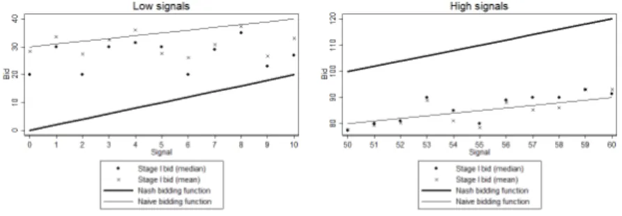
2.4.1 Overall bidding pattern in stage I

Figure 2.2 presents the mean and median bids for low and high signals in stage I. The average bids for low signals are above the Nash prediction and the average bids for high signals are below the Nash prediction in stage I. For high signals the mean and median bids are fitted very well by the na¨ıve bidding function

b^{N V E}_i

(x

i

) =

xi

+ 30.

The results of a Wilcoxon sign rank test show that for high signals the hypothesis that the actual bids are equal to bids resulting from the na¨ıve bidding function cannot be rejected (p = 0.624).

²⁸

26Eyster and Rabin(2005) argued that cursed equilibrium is basically not defined for sequential games and that players in sequential games might be less “cursed” than in simultaneous games.

However, in my setup the players only observe whether their bid was higher or lower than the bid of the opponent, but they do not observe the specific action of the other player, as, for example, in an ascending bid auction. Additionally, it can be argued that the concept of “cursedness” would be a rather weak one if “cursedness” would suddenly vanish in the moment of revealing the other player’s action (see alsoDeversi, Ispano, and Schwardmann(2018)).

27When I compare the effects between INF and NOINF, for different constellations of signal and information, I look at those subjects in treatment NOINF whowould havereceived the respective information if they had been in treatment INF, in order to get an appropriate control group.

28Graphs reporting all bids in stage I and II can be found in AppendixA(Distribution of bids).

Figure 2.2: Median and mean bids in stage I

Overall, we can observe a high occurrence of the winner’s curse for low signals (16.67% in stage I) and of the loser’s curse for high signals (17.02% in stage I).

Conditional on winning, the rate for the winner’s curse increases to 59.31% for low signals and conditional on losing, the rate for the loser’s curse increases to 56.47%

for high signals. The rate of the winner’s curse is very high, especially when consid- ering that the auctions were conducted as second-price auctions. This shows clearly that the problem of irrational bidding behavior is a considerable one. A further conclusion is that emotional factors of winning seem to play a minor role in stage I, since the rates for winner’s and loser’s curse are very similar.

Low(LOST) Low(WON) Low High(LOST) High(WON) High

No curse 338 59 397 74 378 452

91.11% 40.69% 76.94% 43.53% 95.94% 80.14%

Winner’s curse 0 86 86 0 16 16

0.00% 59.31% 16.67% 0.00% 4.06% 2.84%

Loser’s curse 33 0 33 96 0 96

8.89% 0.00% 6.40% 56.47% 0.00% 17.02%

Total 371 145 516 170 394 564

100.00% 100.00% 100.00% 100.00% 100.00% 100.00%

Table 2.2: Winner’s curse and loser’s curse in Stage I for different constellations of signals. Winner’s curse: won, but with a negative payoff. Loser’s curse: lost, but could have won the auction with a positive payoff.

2.4.2 Bidding behavior in stage II

In this subsection, I present an analysis of the difference in bidding behavior be-

tween stage I and II and across treatments. First, I will illustrate my findings by