Inauguraldissertation zur
Erlangung des Doktorgrades der
Wirtschafts- und Sozialwissenschaftlichen Fakultät der
Universität zu Köln 2014
vorgelegt von
Dipl. Math. Johannes Kern aus
Villingen-Schwenningen
Tag der Promotion: 10.7.2014
stellung dieser Arbeit geholfen haben. Insbesondere
• Carlos Alós-Ferrer für die erstklassige Betreuung,
• Klaus Ritzberger für die Erstellung des Zweitgutachtens,
• Ðura-Georg Granić für mehrfaches Korrekturlesen, gute Kommentare und moralische Unterstützung,
• Johannes Buckenmaier, Jaume García-Segarra, Sabine Hügelschäfer, Ana Križić, Jiahui Li, Alexander Ritschel, Fei Shi und Alexander Wag- ner für die tolle Zusammenarbeit während der letzten Jahre,
• meiner Mutter Hildegard Kern sowie Verena Kempf für die Unter-
stützung während der letzten Jahre.
List of Tables v
List of Figures vi
Introduction and Summary 1
1 Repeated Games in Continuous Time as Extensive Form Games 5
1.1 Introduction . . . . 5
1.2 Repeated Games in Continuous Time . . . . 9
1.2.1 Extensive Form Games Without Discreteness Assump- tions . . . . 9
1.2.2 Existing Approaches to Extensive Form Games in Con- tinuous Time . . . 13
1.2.3 The Action-Reaction Framework . . . 15
1.3 A Possibility Result . . . 22
1.3.1 Strategies and Outcomes in General Extensive Form Games . . . 23
1.3.2 Strategies and Outcomes in the Action-Reaction Frame- work . . . 25
1.4 An Alternative Approach: Strategy Constraints . . . 26
1.5 An Equivalence Result . . . 31
1.5.1 Outcome-Equivalence and Equivalence Classes . . . 31
1.5.2 Equivalence of CRM and Action-Reaction Framework . 34 1.6 Relation to the Literature . . . 36
1.6.1 Maximal Strategy Sets . . . 36
1.6.2 Staying Quiet . . . 38
ii
Appendix 1.B: Proofs from Section 1.4 . . . 51
Appendix 1.C: Proofs from Section 1.5 . . . 58
Appendix 1.D: Proposition 5 . . . 76
References Chapter 1 . . . 77
2 Comment on “Trees and Extensive Forms” 81 2.1 Introduction . . . 81
2.2 Preliminaries . . . 81
2.3 Corrected Formulation and Changes . . . 82
2.4 Example . . . 86
References Chapter 2 . . . 88
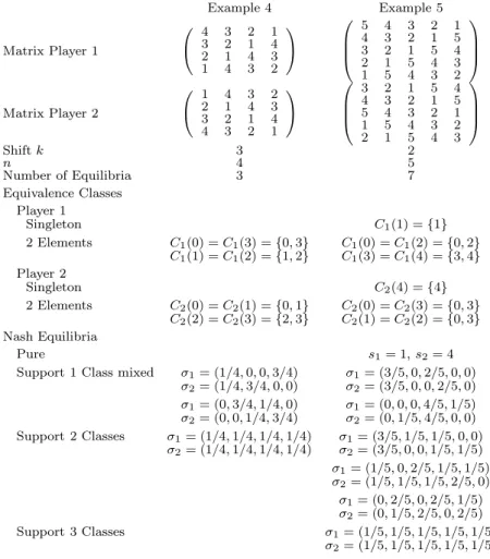
3 Circulant Games 89 3.1 Introduction . . . 89
3.2 Circulant Games . . . 92
3.3 Main Results . . . 97
3.3.1 Preliminaries . . . 97
3.3.2 The Number of Nash Equilibria . . . 99
3.3.3 The Structure of Nash Equilibria . . . 100
3.4 Generalizations . . . 103
3.5 Conclusion . . . 104
Appendix 3.A: Transformation of Games . . . 106
Appendix 3.B: Proofs of Main Results . . . 107
Appendix 3.C: Tables . . . 119
References Chapter 3 . . . 121
4 Preference Reversals: Time and Again 123 4.1 Introduction . . . 123
4.2 A Simple Model of Preference Reversals and Decision Times . 126 4.2.1 Model and Rationale . . . 127
4.2.2 Predictions . . . 129
4.3.1 Experimental Design and Procedures . . . 136
4.3.2 Procedures . . . 138
4.3.3 Results of Experiment 1 . . . 139
4.3.4 Regression Analysis for Experiment 1 . . . 142
4.3.5 Discussion of Experiment 1 . . . 146
4.4 Experiment 2: Eliminating Reversals . . . 147
4.4.1 Motivation and Hypotheses . . . 147
4.4.2 Design of Experiment 2 . . . 148
4.4.3 Procedures . . . 150
4.4.4 Results of Experiment 2 . . . 150
4.4.5 Regression Analysis for Experiment 2 . . . 156
4.4.6 Discussion of Experiment 2 . . . 158
4.5 General Discussion and Conclusion . . . 161
Appendix 4.A: Proofs . . . 163
Appendix 4.B: Lotteries . . . 168
Appendix 4.C: Screenshots . . . 169
References Chapter 4 . . . 170
iv
3.1
Examples of iso-circulant games.. . . 119
3.2
Examples of counter-circulant games.. . . 120
4.1
Preference reversal rates, Experiment 1.. . . 139
4.2
Random effects panel regressions for decision times, Experiment 1.144
4.3
Preference reversal rates, Experiment 2.. . . 151
4.4
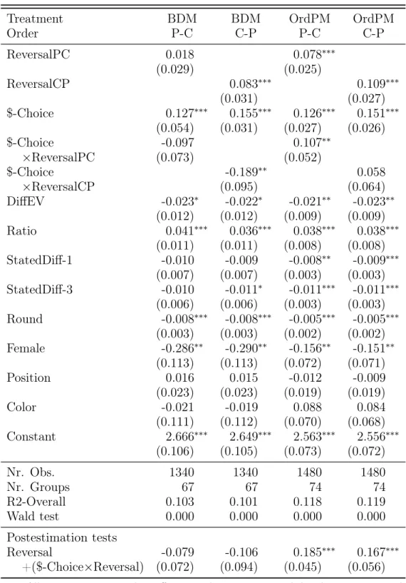
Random effects panel regressions for decision times, Experiment 2.157
4.5
The lottery pairs.. . . 168
4.1
Average number of reversals per subject, Experiment 1.. . . 140 4.2
Average decision time per individual in the choice task, Experiment 1.141 4.3
Average non-reversal decision time per individual in the choice task,Experiment 1.
. . . 143 4.4
Average number of reversals per subject, Experiment 2.. . . 152 4.5
Average decision time per individual in the choice task, Experiment 2.154 4.6
Average non-reversal decision time per individual in the choice task,Experiment 2.
. . . 155 4.7
Screen displays.. . . 169
vi
This dissertation consists of four research papers, covering topics from decision and game theory. Chapters 1 and 2 concern continuous-time games and extensive forms. Chapter 3 presents results on the number of Nash equilibria in a particular class of games called circulant games, while Chapter 4 covers the preference reversal phenomenon. In the following, I present a brief overview of the four chapters summarizing the main findings.
Chapter 1, entitled “Repeated Games in Continuous Time as Extensive
Form Games”, is the result of joint work with Carlos Alós-Ferrer (University
of Cologne). Continuous-time games suffer from a severe conceptual issue,
namely that some strategy profiles induce multiple outcomes while other
profiles induce no outcome at all. Since preferences are defined on the set
of ultimate outcomes, neither profiles leading to a multiplicity of outcomes
nor profiles that “evaporate” can be evaluated, hence making it impossible
to analyze such games for example in terms of equilibria. The literature
has proposed several ways to deal with this issue. The most common one
requires players to stick to a chosen action for some strictly positive amount
of time. Indeed, it can be shown that any profile of such strategies induces
a unique outcome. This approach is, however, problematic from a game-
theoretic point of view. Fixing the extensive form of the game (i.e. decision
nodes and choices) determines the players’ strategies as these are mappings
from the set of decision nodes to the set of choices. Placing exogenous re-
strictions on the set of strategies hence implicitly changes (and in the worst
case destroys) the extensive form. Our paper presents a game-theoretically
well-founded framework for modeling repeated games in continuous time. It
further provides a clarification as to which restrictions on strategies can be
allowed in the sense that the resulting strategies can be derived from a well-
defined extensive form. Work on this paper was shared among authors as
follows: Johannes Kern 50%, Carlos Alós-Ferrer 50%.
nal of Economic Theory, Vol. 146, No. 5, September 2011, pp. 2165–2168.
The paper comments on the definition of Extensive Form in Alós-Ferrer and Ritzberger (2008) and shows that one of the properties there needs to be ad- justed. It provides counterexamples showing that with the original version of this property some results do not hold as stated and presents a corrected formulation of the property as well as the corrected statement of the results.
It further provides proofs for these results under the new formulation. Work on this paper was shared among authors as follows: Johannes Kern 33
13%, Carlos Alós-Ferrer 33
13%, Klaus Ritzberger 33
13%.
Chapter 3 entitled “Circulant Games” is joint work with Ðura-Georg Granić (University of Cologne). Games with a cyclical structure are ubiq- uitous in game theory and are routinely used to generate popular examples, starting with Matching Pennies and Rock-Paper-Scissors. For these as well as larger games, the cyclical structure can be captured by circulant payoff matrices in which each row vector is rotated by one element relative to the preceding row vector. In our paper we study a class of two-player games in which both players payoffs are given by such circulant matrices. Given that these payoffs are ordered, we are able to determine the exact number of (pure and mixed) Nash equilibria. This number only depends on the number of strategies, the position of one of the player’s largest payoff in the first row of his payoff matrix, and whether the players’ payoff matrices “cycle” in the same or in different directions. Our results further allow us to describe the support of each Nash equilibrium strategy. Work on this paper was shared among authors as follows: Johannes Kern 50%, Ðura Georg Granić 50%.
Chapter 4, “Preference Reversals: Time and Again”, is the result of joint work with Carlos Alós-Ferrer, Ðura-Georg Granić, and Alexander K. Wagner (all at the University of Cologne). Experiments documenting the preference reversal phenomenon highlight that, contrary to the invariance assumption underlying most economic theories of choice, preferences may actually be in- fluenced by the elicitation method employed. In the most basic setup of such
2
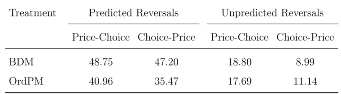
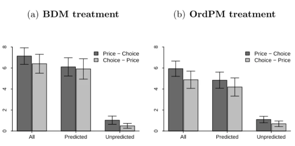
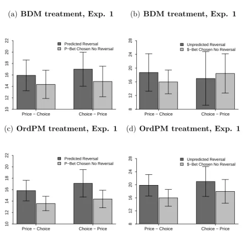
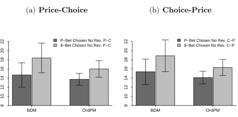
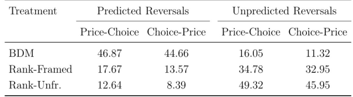
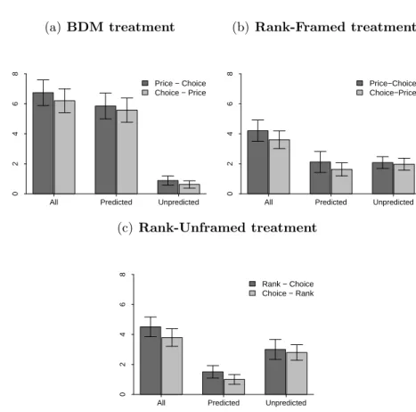
($-bet). They are then asked to state prices for each of the lotteries. A prefer- ence reversal occurs if either the $-bet receives a higher price in a pair where the P -bet is chosen (predicted reversal) or the P -bet receives a higher price in a pair where the $-bet is chosen (unpredicted reversal). The preference re- versal phenomenon is characterized by a significantly higher rate of predicted reversals. We present a new, simple process-based model that explains the preference reversal phenomenon and makes novel predictions about the asso- ciated decision times in the choice phase. The phenomenon is jointly caused by noisy lottery evaluations and an overpricing phenomenon associated with the compatibility hypothesis. A laboratory experiment confirmed the model’s predictions for both choice data and decision times. Choices associated with reversals take significantly longer than non-reversals, and non-reversal choices take longer whenever long-shot lotteries are selected. A second experiment showed that the overpricing phenomenon can be shut down, greatly reducing reversals, by using ranking-based, ordinally-framed evaluation tasks. This experiment also disentangled the two determinants of the preference rever- sal phenomenon since noisy evaluations still deliver testable predictions on decision times even in the absence of the overpricing phenomenon. Work on this paper was shared among authors as follows: Johannes Kern 25%, Carlos Alós-Ferrer 25%, Ðura Georg Granić 25%, Alexander K. Wagner 25%.
References
Alós-Ferrer, C.,
andK. Ritzberger (2008): “Trees and Extensive
Forms,” Journal of Economic Theory, 43(1), 216–250.
Extensive Form Games
1.1 Introduction
Suppose two players play a continuous-time version of the infinitely repeated Prisoner’s Dilemma, starting at time t = 0. A player is then free to choose a strategy conditioning on arbitrary events in the past. For instance, a player could specify the following grim-trigger strategy: cooperate as long as both players have always cooperated in the past, otherwise defect forever. Now suppose both players use this strategy. One is tempted to conclude that the outcome of the strategy profile is eternal cooperation. Indeed, this outcome is compatible with the strategy profile in the sense that, at every point in time, instantaneous cooperation is prescribed by the strategy profile given the past history contained in the outcome. However, if time is continuous, there are infinitely many other outcomes which are equally compatible with these grim-trigger strategies. Fix any arbitrary time T , and consider the outcome where both players cooperate up to and including time T , and defect at any later point in time. Since there is no first point in time where players defect, this outcome never contradicts the prescriptions of the grim- trigger strategy profile and hence is also compatible with it. We conclude that the strategy profile induces a continuum of different outcomes. As a consequence, even if every outcome has a well-defined payoff, the payoff of the considered strategy profile is not well-defined, and a game-theoretical analysis becomes impossible.
Outcome multiplicity is not the only problem in continuous-time repeated
games. Consider a different strategy profile where each player starts coop-
erating and further decides to cooperate unless only cooperation has been
cannot be the outcome. But, if a defection occurred at any strictly posi- tive point in time, this must mean that no defection occurred before, and hence the strategies prescribe a defection at every previous, strictly positive point in time, a contradiction. Hence, this simple strategy profile induces no outcome at all.
These problems have been previously pointed out by Anderson (1984), Simon and Stinchcombe (1989), Stinchcombe (1992), and Alós-Ferrer and Ritzberger (2008), among others. As shown in Alós-Ferrer and Ritzberger (2008, 2013a), they are not exclusive of continuous-time settings: intuitively, it suffices for the time axis to have an accumulation point towards the past to generate such problems, as e.g. in the case of the time set {1/n}
n=1,2,...S
{0}.
We now have a good understanding of the underlying reasons for these prob- lems. Alós-Ferrer and Ritzberger (2008) (see also Alós-Ferrer, Kern, and Ritzberger, 2011) formulated out a characterization of the set of extensive forms where every profile of pure strategies generates a unique outcome (and hence a normal-form game can be defined). This characterization can be ar- gued to describe the domain of game theory, for games outside the character- ized set cannot be “solved” in any sense of the word. Unsurprisingly, perfect- information continuous-time games are outside this domain; technically, they fail a condition called “up-discreteness” in Alós-Ferrer and Ritzberger (2008), which precludes accumulation points toward the past.
This state of affairs has not prevented economic theory from venturing into the realm of continuous-time games (the literature is of course too ex- tensive to review it here). And neither should it. On the one hand, contin- uous time is often analytically convenient due to the possibility of employ- ing techniques from differential calculus along the time dimension. On the other hand, discrete time sometimes creates artificial phenomena which van- ish away in continuous time; and it is their vanishing in the latter framework which proves their artificiality in the former. However, the problems pointed out above create serious difficulties with the interpretation of continuous- time applications. For instance, if certain strategy combinations fall out of the framework by virtue of creating outcome existence or uniqueness prob-
6
lems, the meaning of any equilibrium concept becomes questionable, since some deviations might be excluded for merely technical reasons, and not the self-interest of the deviator. Further, if a proper extensive form game can- not be specified for a continuous-time model, notions of “time consistency”
cannot rely on subgame perfection or other equilibrium refinements based on backward induction, since in the absence of a properly formulated extensive form, it is not possible to determine the full collection of subgames capturing the strategic, intertemporal structure of the problem.
One typical approach for developing a coherent framework in continuous time is to admit an exogenous restriction on the set of pure strategies and de- clare some of those inadmissible. In the case of differential games (Friedman, 1994), this approach often leads to the specification of a normal-form game, where strategies are required to be e.g. differentiable or integrable functions of some state variable. In other domains, the analysis has been restricted to strategies incorporating some Markov structure, as e.g. in the case of the literature on (individual) strategic experimentation (e.g. Keller and Rady, 1999; Keller, Rady, and Cripps, 2005). The approach was most effectively described by Stinchcombe (1992), who set out to identify a maximal set of strategies for a continuous-time game such that every strategy profile induces a unique outcome. The result incorporates elements of a framework intro- duced by Anderson (1984) and also studied by Bergin and MacLeod (1993) and Bergin (1992, 2006), and rests on the condition that a strategy must always identify the player’s next move.
Stinchcombe (1992) identifies the best that can be done through strategy
constraints once one accepts the inconvenient fact that unconstrained con-
tinuous time games cannot be solved. From a game-theoretic point of view,
however, restricting the strategy set is an unsatisfactory approach. On the
one hand, since certain strategies are excluded on purely technical grounds,
we face the problems with the interpretation of equilibria and time consis-
tency pointed out above. On the other hand, there is a more fundamental,
conceptual problem. An extensive form game incorporates a complete de-
scription of the possible choices of every player at every decision node. A
behavioral strategy is merely a collection of possible “local” decisions at the
nodes, and any possible combination thereof is a feasible behavioral strategy.
Once the game is specified, there can be no further freedom in the specifica- tion of the possible local decisions, since those have already been fixed in the extensive form. The set of possible behavioral strategies is thus automatically specified once the extensive form is given.
A restriction prohibiting a given combination of local decisions in order to preserve some property of the outcome, no matter how desirable, lacks any decision-theoretic justification. Worse, it is then unclear whether the extensive form structure survives the restriction, raising doubts as to whether the resulting formal object is simply a (constrained) normal-form game.
Here we propose a different approach to the study of continuous-time games. The basic idea is as follows. Continuous time is a convenient device;
its modelization within an extensive form game, however, needs only go so far as it is useful for game-theoretic purposes. The formalizations analyzed until now might have “gone too far”, in the sense that the associated extensive forms become too large and restoring tractability requires restricting their strategy spaces. The literature has concentrated on providing ideas and rationales for restricting the strategy space in an ex-post way. In this paper, we prove that continuous-time decisions can be captured by applying those ideas to the very definition of the game. The resulting formal object can then still be considered a well-defined “continuous-time game”; it is, however, a fully solvable extensive form game, i.e. every strategy profile induces a unique profile, without any restriction on the set of behavioral strategies.
The advantage is that the framework is an extensive form game without any caveat, and standard game-theoretic concepts and methods can then be applied. In other words, our message is a positive one: we show that continuous-time modeling is possible without giving up the benefits and the conceptual discipline resulting from well-defined extensive form games.
In this paper, we focus on the repeated-game framework with observable actions.
1Specifically, we show how repeated games in continuous time can
1This is the framework where the problems we mentioned above are the most severe.
Continuous-time models are also customarily used in different frameworks, e.g. games with imperfect monitoring (Sannikov, 2007). Intuitively, the fact that players cannot condition on as many events as in the case of perfectly observable actions shrinks the strategy space
be formalized incorporating natural conditions from the onset. The construc- tion is not trivial, and in order to describe it we must carefully detail the appropriate game tree and choice structure. Once this is in place, we show that, by virtue of fulfilling the appropriate conditions, the resulting game is well-behaved without any restrictions on the strategy sets. In order to link our construction to the literature, we then show that it is possible to retrace our steps and prove an equivalence result between the unrestricted behav- ioral strategies in our repeated game and a restricted class of strategies in a more naïvely specified (and hence, in our view, problematic) continuous-time repeated game.
The paper is structured as follows. Section 1.2 lies out the general frame- work for repeated games in continuous time, the Action-Reaction Framework.
Section 1.3 presents our main result, showing that in our framework all strat- egy profiles induce unique outcomes. Section 1.4 presents the alternative ap- proach through restricted strategies (Conditional Response Mappings) and Section 1.5 proves an equivalence result, which allows us to link our exten- sive form to the previous literature in Section 1.6. Section 1.7 concludes.
The construction and the main arguments are detailed in the main text but specific proofs are relegated to the appendix.
1.2 Repeated Games in Continuous Time
1.2.1 Extensive Form Games Without Discreteness As- sumptions
Working definitions of extensive form games frequently incorporate strong re- strictions in the form of explicit finiteness or discreteness assumptions. Since we aim to view continuous-time repeated games as extensive form games, we need a more general approach. We will rely on a definition of extensive form games allowing for infinite time horizon, continuous time axis, and arbitrary action sets. This concept is the basis for a general framework developed in
and makes it easier to obtain a well-defined extensive form game. See Alós-Ferrer and Kern (2013) for a comment.
Alós-Ferrer and Ritzberger (2005, 2008, 2013a,b).
The definition comes in two parts. The first is a general concept of game tree, capturing the order and nature of decisions. The second is a definition of extensive decision problem (given the game tree) which incorporates all appropriate consistency conditions on the choices that players can make.
Let us start with game trees. Following Kuhn (1953), a game tree is just an ordered set of “decision points” or nodes which can be represented as an abstract graph. Alternatively, von Neumann and Morgenstern (1944) focus on ultimate outcomes as the primitive objects and consider nodes as sets of such outcomes, which become finer as decisions are taken. A result arising in the work quoted above is that there exists exactly one way of defining game trees such that both approaches are equivalent. As a consequence, there is no loss of generality in assuming a game tree where nodes are taken to be sets of ultimate outcomes, as in the following definition.
Definition 1. A (rooted) game tree T = (N, ⊇) is a collection of nonempty subsets x ∈ N (called nodes) of a given set W partially ordered by set inclusion such that W ∈ N (W is called the root) and
(TI) “Trivial Intersection:” if x, y ∈ N with x ∩ y 6= ∅, then x ( y or y ⊆ x.
(IR) “Irreducibility:” if w, w
′∈ W with w 6= w
′, then there exist x, x
′∈ N such that w ∈ x \ x
′and w
′∈ x
′\ x.
(BD) “Boundedness:” for every nonempty chain h ⊆ N there exists w ∈ W such that w ∈ x for all x ∈ h.
2A play is a chain of nodes h ⊆ N that is maximal in N , i.e. there is no x ∈ N \ h such that h ∪ {x} is a chain. Plays are the natural objects on which preferences can be defined in a setting where the time horizon is not assumed to be finite. The advantage of game trees is that the underlying set W can also be identified with the set of plays. Specifically, Alós-Ferrer and Ritzberger (2005, Theorem 3(c)) show that an element w ∈ W can be seen either as a possible outcome (element of some node) or as a play (maximal
2A chain is a subset ofN that iscompletely ordered by set inclusion.
chain of nodes), and a node x ∈ N can be identified with the set of plays passing through it.
For a game tree (N, ⊇) with set of plays/outcomes W and an arbitrary subset a ⊆ W (not necessarily a node), define the up-set ↑ a and the down-set
↓ a by
↑ a = {y ∈ N |y ⊇ a } and ↓ a = {y ∈ N |a ⊇ y } .
The key implication of (TI) is that ↑ x is a chain for all x ∈ N , which is contained in (can be “prolonged to”) the play ↑ {w} for any w ∈ x. Further, if h is a play, by (BD) there exists a unique outcome w ∈ W such that
∩
x∈hx = {w}, or, equivalently, h =↑ {w}. This fact is the basis for the equivalence between outcomes and plays, which essentially reduces to the fact that, for w ∈ W and x ∈ N, w ∈ x if and only if x ∈↑ {w}. When a distinction is called for, we write w for the outcome and ↑ {w} for the play (chain of nodes).
We now turn to the second part of the definition. In an extensive form game, players make decisions at nodes that are properly followed by other nodes, called moves. Let X = {x ∈ N | ↓x \ {x} 6= ∅ } be the set of all moves.
3In finite, perfect information examples, the possible actions or op- tions available to a player at a given move can be identified with the nodes following that move (its immediate successors). In more general settings, we need a more general object. The possible alternatives faced by players are modeled through choices, which are subsets c ⊆ W satisfying a number of consistency conditions.
Before we present those conditions, we need a notion of when a choice c is available at a move x. For an arbitrary set of outcomes/plays a ⊆ W , the set of immediate predecessors of a is defined by
P (a) = {x ∈ N |∃y ∈↓ a : ↑ x =↑ y\ ↓ a } .
Since nodes in a game tree are sets of plays, they too may, but need not, have immediate predecessors. Since choices are also sets of plays, the set of
3All other nodes are calledterminal. It follows from (IR) that a nodex∈N is terminal if and only if there is w∈W such thatx={w}.
immediate predecessors of a choice is well defined, and we will say that a choice c is available at a move x ∈ X if x ∈ P (c). This is the key element in the following definition.
Definition 2. An extensive decision problem (EDP) with player set I is a pair (T, C ), where T = (N, ⊇) is a game tree with set of plays W and C = (C
i)
i∈Iis a system consisting of collections C
i(the sets of players’
choices) of nonempty unions of nodes (hence, sets of plays) for all i ∈ I such that
(EDP.i) if P (c) ∩ P (c
′) 6= ∅ and c 6= c
′, then P (c) = P (c
′) and c ∩ c
′= ∅, for all c, c
′∈ C
ifor all i ∈ I;
(EDP.ii) x ∩
∩
i∈I(x)c
i6= ∅ for all (c
i)
i∈I(x)∈ A (x) and for all x ∈ X;
(EDP.iii) if y, y
′∈ N with y ∩ y
′= ∅ then there are c, c
′∈ C
ifor some player i ∈ I such that y ⊆ c, y
′⊆ c
′, and c ∩ c
′= ∅;
(EDP.iv) if x ) y ∈ N , then there is c ∈ A
i(x) such that y ⊆ c for all i ∈ I (x), for all x ∈ X;
where A (x) = ×
i∈I(x)A
i(x), A
i(x) = {c ∈ C
i|x ∈ P (c) } are the choices available to i ∈ I at x ∈ X, and I (x) = {i ∈ I |A
i(x) 6= ∅ } is the set of decision makers at x, which is required to be nonempty, for all x ∈ X.
An extensive form game is an extensive decision problem together with a specification of players’ preferences on the set of plays.
The interpretation of the conditions above is as follows (see Alós-Ferrer
and Ritzberger, 2005, Section 5 or Alós-Ferrer and Ritzberger, 2008, Section 3
for additional details). (EDP.i) stands in for information sets: if two distinct
choices c, c
′∈ C
iare ever simultaneously available, then they are disjoint
and available at the same moves—at those in the information set P (c) =
P (c
′). (EDP.ii) requires that simultaneous decisions by different players
at a common move do select some outcome. (EDP.iii) states that for any
two disjoint nodes, there is a player who can eventually make a decision that
selects among them. Finally, (EDP.iv) states that, if a player takes a decision
at a given node, he must be able not to discard any given successor of the
node. This excludes absent-mindedness (Piccione and Rubinstein, 1997), as
in the original formulation of Kuhn (1953).
An important point about EDPs is that they allow several players to de- cide at the same move. This sometimes simplifies both the representation of a game and the equilibrium analysis (see Alós-Ferrer and Ritzberger, 2013a, for examples). This will also be important for our present purposes, for in repeated games players act simultaneously at every time point. If we adopted the convention that each move is assigned to one player only, we would be forced to incorporate artificial “cascading information sets” to accommodate this characteristic.
1.2.2 Existing Approaches to Extensive Form Games in Continuous Time
We now turn to the specific problem of modeling a repeated game in contin- uous time explicitly as an extensive form game. A first, direct approach to this task is to define strategies as mappings from the set of history-time pairs to the set of possible actions with the minimal requirement that at time t the same action is prescribed for two histories that agree on [0, t[. Indeed, this approach can be readily formalized as an EDP (Alós-Ferrer and Ritzberger, 2005, 2008).
Let W be the set of functions f : R
+→ A, where A = Q
i∈I
A
iand each A
iis some fixed set of actions containing at least two elements. W is the set of all possible outcomes in the continuous-time repeated game.
Let the set of nodes be N = {x
t(f ) | t ∈ R
+, f ∈ W }, where x
t(f ) = {g ∈ W | g(τ ) = f (τ) ∀ τ ∈ [0, t[ } for f ∈ W and t ∈ R
+. A node x
t(f) contains all functions that agree with f on [0, t[ while all possibilities of val- ues at t and afterwards are still open. (N, ⊇) can be shown to be a game tree (Alós-Ferrer and Ritzberger, 2005).
A strategy in this framework is a mapping assigning a choice of the form
c
it(f, a
i) = {g ∈ x
t(f ) | g
i(t) = a
i} (for some a
i∈ A
i) to every move of the
form x
t(f). However, it is then possible to define strategies like the ones
described in the introduction that induce no outcome or that induce a con-
tinuum of outcomes (cf. Examples 10 and 12 of Alós-Ferrer and Ritzberger,
2008). Hence, this approach, while intuitive, is not suited to model repeated
games in continuous time. In order to be able to “solve” these games, addi- tional assumptions are needed.
A second approach is to view a continuous-time game as the limit of some sequence of discrete-time games and then define continuous-time strategies as limits of sequences of strategies in discrete time. This approach, however, presents difficulties of its own. A particular problem, pointed out by David- son and Harris (1981) and Fudenberg and Levine (1986), is that sequences of discrete time strategies may not possess a limit (the “chattering problem”).
Imagine, for instance, a sequence of discretizations with period length 1/n and discrete-time strategies prescribing to cooperate in periods k/n with k odd and defect in other periods.
A third approach is to restrict the sets of strategies in a game, that is, to impose the exogenous constraint that certain strategies cannot be used for e.g. equilibrium analysis. This allows to identify strategy sets which keep the framework tractable (e.g. guaranteeing existence and uniqueness of out- comes), and hence avoids the problems mentioned above. This approach has been pursued in Anderson (1984), Bergin (1992, 2006), Bergin and MacLeod (1993), Perry and Reny (1993), and Perry and Reny (1994), among others (see also Simon and Stinchcombe (1989) for a combination of this approach and discrete-time approximations). Stinchcombe (1992) investigates maxi- mal strategy sets such that a unique outcome can be assigned to every admis- sible strategy profile, thereby obtaining a setting which is as good as it can be given a potentially problematic extensive form. As mentioned in the in- troduction, this approach presents conceptual problems because (behavioral) strategies are collections of local decisions, and which decisions are feasible should be solely and completely determined by the extensive form. However, it remains an open question whether the maximal strategy set approach can be reconciled with a pure extensive form approach. This would entail finding a new extensive form such that the unconstrained sets of behavioral strategies are equivalent, in a well-defined sense, to the set of constrained strategies.
We will return to this question in Section 1.5.
1.2.3 The Action-Reaction Framework
Our approach to the problem of defining extensive form games in continuous time is different to the ones just mentioned. We will exhibit a specific exten- sive decision problem capturing repeated decisions in continuous time, such that, for every strategy profile, one and only one associated outcome exists.
The basic construction relies on ideas present in the frameworks of Anderson (1984), Stinchcombe (1992), and Bergin (2006). However, the approach is different at a basic level because strategy sets are kept unconstrained; the differences with respect to the “direct approach”-EDP mentioned above are built directly into the construction of the extensive decision problem.
The basic idea of the construction is as follows. At time 0 all players choose a first action that they will have to stick to for some positive amount of time. This amount of time is determined by the choice of “inertia times”
during which a player is committed to her current action. After this, when- ever a player’s inertia time has run out she can revise her previous action.
If she switches to a different one, i.e. “makes a jump”, the players who did not jump can react instantly and choose new actions as well. All players will again have to stick to their new actions for some positive amount of time, i.e. decide on new inertia times. This construction prevents players from jumping again right after an action change and from reacting even though no other player has jumped. The latter is crucial: a direct consequence is that the set of decision points becomes well-ordered, hence eliminating the problems of the direct approach.
We proceed in two steps. First we will describe the set of outcomes/plays of the game. The construction of this set already incorporates the essence of the Action-Reaction Framework. The second step is to appropriately define nodes and choices and show that the resulting structure is indeed an extensive decision problem.
The Outcome Space
Fix a finite set of players I and an arbitrary action space A
ifor each player
i ∈ I. Assume that A
iis a metric space.
We start by defining the set of plays, i.e. the possible maximal chains of decisions that might actually occur during the game. Ultimately, the history of all decisions taken by a player i builds a function f
i: R
+7→ A
ias in the direct approach. We will introduce additional constraints to reflect the Action-Reaction Framework.
We require some preliminary notation. First, given a metric space B, call a function g : R
+7→ B (right-)piecewise constant if for every t ∈ R
+there exists ε > 0 such that g
]t,t+ε[is constant. If g is piecewise constant, g
+(t) := lim
τ→t+g(τ ) exists for all t ∈ R
+. In this case, define
RK(g) = {t ∈ R
+| g
+(t) = g(t) }
to be the set of points where g is right-constant. Second, given any function g : R
+7→ B, let
LC (g) =
t ∈]0, +∞[
∃ g
−(t) := lim
τ→t−
g(τ) ∧ g
−(t) = g(t)
denote the set of points where g is left-continuous.
4The following definition spells out the first ingredient of our framework.
Definition 3. A decision path is a tuple f = (f
i)
i∈Isuch that (DP.i) for each i ∈ I , f
i: R
+7→ A
iis piecewise constant,
(DP.ii) for each i ∈ I , LC (f
i) S
RK (f
i) = R
+,
(DP.iii) for each t ∈ R
+, if ∃ i ∈ I with t ∈ R(f
i), then ∃ j ∈ I with t ∈ J (f
j), where J(f
i) := RK (f
i) \ LC(f
i) and R(f
i) := LC (f
i) \ RK (f
i) are the set of jump points and reaction points of player i, respectively. The set of all decision paths is denoted by F .
Property (DP.i) states that a player’s action revision cannot occur arbi- trarily close to a previous action revision. A direct consequence (see Lemma
4For piecewise constant functions as defined here, a function is right-continuous attif and only if it is right-constant att.
A.2 in Section 1.7) is that the set of jump points of any player is well-ordered by the usual order on the real numbers. Property (DP.ii) requires that a player’s action revision cannot take the form of an instantaneous change which is then abandoned (i.e. simultaneous failure of left- and right-continui- ty).
5Taken together, (DP.i) and (DP.ii) mean that when a player changes action, be it due to a jump or to a reaction to somebody else’s revision, the player is not able to change action again immediately after the change.
Property (DP.iii) is the only condition requiring consistency across play- ers’ paths of decisions. Intuitively, jump points are those where a players’
decision path has changed discontinuously (a sudden action revision), while t is a reaction point if the player’s strategy shifts immediately after t but not at t, in reaction to an observed shift of another player at t: an “instant reaction”. (DP.iii) states that a player can change action by instant reaction only if some other player jumped at t.
The second key ingredient of the Action-Reaction Framework are inertia times. By (DP.i), after every jump or reaction at t, there exists ε > 0 such that the player is “committed” not to revise action again until at least t + ε (although a better interpretation is a physical impossibility to revise too often). We will introduce an explicit record of inertia times as part of every play. Formally, let E be the set of all possible functions ǫ = (ǫ
i)
i∈Iwith ǫ
i: R
+→ R
+such that ǫ
i(0) > 0 for all i ∈ I. The quantity ǫ
i(t) will play the role of a marker, with the interpretation that ǫ
i(t) > 0 if and only if player i is able to revise her action at t. In that case, ǫ
i(t) represents the length of time after t for which player i cannot change action again, unless it is as reaction to some other action change.
Define the set of decision points of player i as DP (ǫ
i) := {t ∈ R
+| ǫ
i(t) > 0 } ,
i.e. the set of times at which player i is able to take a decision. In order to link inertia times with decision paths, we will have to spell out consistency
5In particular, (DP.ii) implies that 0∈RK(fi)for alli∈I, i.e.f+(0) =f(0). That is the players’ initial decisions cannot be adjusted arbitrarily close to t= 0. Note that this implies0∈RK(fi)\LC(fi) =J(fi)for alli∈I.
conditions. A minimal such condition is that J (f
i) ∪ R(f
i) ⊆ DP (ǫ
i), i.e.
whenever a player makes a decision or reacts to another decision at time t, an inertia time ǫ
i(t) > 0 is specified. However, the inclusion will typically be strict, since a player can always decide to keep the previous action, which still requires specifying a (new) inertia time. That is, t ∈ DP (ǫ
i) indicates a decision which might not be observable as such (because no action change ensues), while t ∈ J(f
i) ∪ R(f
i) implies an observable action change.
Before introducing the announced consistency conditions, again we re- quire additional notation. Since ǫ
i(0) > 0, for all i ∈ I, ǫ ∈ E, and t ∈]0, +∞[
the intersection DP (ǫ
i) ∩ [0, t[ is not empty and hence by the Supremum Ax- iom we can define
Prev(ǫ
i, t) := sup(DP (ǫ
i) ∩ [0, t[),
which gives the last time before t that player i has taken a decision. Define Prev(ǫ
i, 0) = 0 for all i ∈ I and ǫ ∈ E. For i ∈ I , ǫ ∈ E, and t ∈ DP (ǫ
i) define
Next(ǫ
i, t) := t + ǫ
i(t),
which gives the next time after t that player i can initiate an action change if no other player jumps before. Further let
P J(ǫ
i) := {t ∈ R
+| Next(ǫ
i, Prev(ǫ
i, t)) = t } ∪ {t ∈ R
+| t = Prev(ǫ
i, t)}
be the set of potential jumps for player i, i.e. the set of times where a player is allowed to initiate an action change according to the inertia times. Those are of two kinds. The “natural ones” are those where the inertia time since the last time an action change was implemented has “run out”. The second is slightly counterintuitive, and corresponds to points which are the supremum of the set of prior time points where action changes have been initiated, i.e.
accumulation points of prior action changes.
Last, for w = (f, ǫ) ∈ F × E and t ∈ R
+define (for notational conve-
nience) IDP (ǫ, t) := {i ∈ I | t ∈ DP (ǫ
i)}, IJ(f, t) := {i ∈ I | t ∈ J(f
i)},
and IP J (ǫ, t) := {i ∈ I | t ∈ P J (ǫ
i) }, i.e. the sets of players having decision
points, jumps, and potential jumps at t, respectively.
We are now ready to define the set of plays, which incorporate the con- nection between decision paths and inertia times.
Definition 4. A play is a pair w = (f, ǫ) ∈ F × E such that (P.i) for each i ∈ I, J (f
i) ⊆ P J(ǫ
i);
(P.ii) for each i ∈ I, J (f
i) ⊆ T
j∈I
DP (ǫ
j);
(P.iii) for each i ∈ I, P J (ǫ
i) ⊆ DP (ǫ
i);
(P.iv) for each i ∈ I and each t ∈ DP (ǫ
i) if τ ∈ DP (ǫ
i)∩]t, Next(ǫ
i, t)[ then S
j6=i
J(f
j)∩]t, τ ] 6= ∅.
The set of all plays is denoted by W .
(P.i) states that a player can jump at t only if t was indeed a potential jump. (P.ii) means that, whenever a player jumps, every player who does not also jump is allowed to react, and all players have to specify inertia times. Note that (P.ii) together with (DP.iii) implies that J (f
i) ∪ R(f
i) ⊆ DP (ǫ
i). (P.iii) requires that every potential jump be a decision point. The interpretation of (P.iv) is as follows. If at time t a player makes a decision with inertia time ε, then the only way he can make a decision before t + ε is if some other player jumped before t + ε.
The Extensive Decision Problem
We first define the decision nodes, and hence the tree.
For every w = (f, ǫ) ∈ W and t ∈ R
+, define the following sets x
t(w) = {w
′= (f
′, ǫ
′) ∈ W | w
′(τ) = w(τ) ∀ τ ∈ [0, t[ } , x
Rt(w) = {w
′= (f
′, ǫ
′) ∈ x
t(w) | f
′(t) = f (t)} ,
x
Pt(w) =
w
′= (f
′, ǫ
′) ∈ x
Rt(w)
f
+′(t) = f
+(t) .
Nodes of the form x
t(w) are “potential jump nodes” at which a player
might make the decision to initiate a change of action. Hence, they will
be part of the tree whenever t ∈ S
i∈I
P J(ǫ
i) or, equivalently, whenever IP J (ǫ, t) 6= ∅.
Nodes of the form x
Rt(w) are “reaction nodes” which model the possibility of players to react to a change of action initiated by another player. Hence they are part of the tree whenever t ∈ S
i∈I
J(f
i) but t / ∈ J(f
j) for some j ∈ I; equivalently, whenever ∅ ( IJ (f, t) ( I.
Nodes of the form x
Pt(w) are “peek nodes” where both the actions at t (individual action change initiations) and the immediate reactions to them (the right limits of f ), have already been decided, but the times ǫ
i(t) still have not. Again, they are part of the tree whenever IP J(ǫ, t) 6= ∅.
Note that nodes are independent of the “representant play”. If w
′∈ x
t(w), then x
t(w) = x
t(w
′), and analogously for reaction and peek nodes.
Potential jump, reaction, and peek nodes account for all possible decision situations. Note that the root, i.e. the node W containing all plays, is con- tained in N because x
0(w) = W for all w ∈ W . The root is followed by peek nodes of the form x
P0(w). The set of nodes is given by
N = {x
t(w) | t ≥ 0, IP J(ǫ, t) 6= ∅ }
[ x
Rt(w) | t > 0, ∅ ( IJ(f, t) ( I (1.1) [ x
Pt(w) | t ≥ 0, IP J(ǫ, t) 6= ∅ .
We now specify the choices, and hence the extensive decision problem by reviewing the decisions that have to be taken at each type of node. At potential jump nodes x
t(w), players who are allowed to jump may decide how to continue, i.e. which action to adopt. That is, for every t ≥ 0, w = (f, ǫ) ∈ W , i ∈ IP J (ǫ, t), and a
i∈ A
i, we include the choice
c
i(x
t(w), a
i) = {w
′= (f
′, ǫ
′) ∈ W | t ∈ P J(ǫ
′i), f
′(τ ) = f(τ ) ∀ τ ∈ [0, t[,
f
i′(t) = a
i} .
At reaction nodes x
Rt(w), the players who did not jump decide on their instant
reaction. That is, for every t > 0, w = (f, ǫ) ∈ W with IJ(f, t) 6= ∅,
i ∈ I \ IJ (f, t), and a
i∈ A
i, we include the choice c
i(x
Rt(w), a
i) =
w
′= (f
′, ǫ
′) ∈ W
f
′(τ) = f(τ ) ∀ τ ∈ [0, t], f
i+′(t) = a
i. At peek nodes x
Pt(w), all players who either had a potential jump at t or reacted at t decide how long they are going to stick to their action. That is, for every t ≥ 0, w = (f, ǫ) ∈ W , i ∈ I such that i ∈ IDP (ǫ, t),
6and ε
i∈ R
++, we include the choice
c
i(x
Pt(w), ε
i) = {w
′= (f
′, ǫ
′) ∈ W | f
′(τ) = f(τ ) ∀ τ ∈ [0, t],
f
+′(t) = f
+(t), ǫ
′i(t) = ε
i} . Hence, the set of choices of player i is given by
C
i= {c
i(x
t((f, ǫ)), a
i) | t ≥ 0, i ∈ IP J(ǫ, t), a
i∈ A
i}
[ c
i(x
Rt((f, ǫ)), a
i) | t > 0, i ∈ I \ IJ (f, t), IJ(f, t) 6= ∅, a
i∈ A
i[ c
i(x
Pt((f, ǫ)), ε
i) | t ≥ 0, i ∈ IDP (ǫ, t), ε
i∈ R
++.
Let us now look at information sets. By definition an information set in an EDP is the set of immediate predecessors of a given choice. For a choice c = c
i(x
t(w), a
i) ∈ C
iwith w = (f, ǫ) we obtain
P (c) = {x
t((f
′, ǫ
′)) ∈ N | f(τ ) = f
′(τ) ∀ τ ∈ [0, t[, t ∈ P J(ǫ
′i) } . This means that at a potential jump node x
t(w) a player knows all past actions (i.e. the decision path up to time t) but not the record of inertia times which has led to the particular decision path (with the obvious exception that she knows that the play is such that she is allowed to jump).
For a choice c = c
i(x
Rt(w), a
i) ∈ C
iwith w = (f, ǫ) (which implies i / ∈ IJ (f, t)) we have
P (c) =
x
Rt((f
′, ǫ
′)) ∈ N | f
′(τ) = f(τ ) ∀ τ ∈ [0, t] } ,
6This is equivalent to i∈IP J(ǫ, t)orIJ(f, t)6=∅ (see Lemma A.5 in the appendix).
i.e. at a reaction node x
Rt(w) the player knows the decision path up to and including time t.
Finally, for a choice c = c
i(x
Pt(w), ε
i) ∈ C
iwith w = (f, ǫ) we obtain P (c) =
x
Pt((f
′, ǫ
′)) ∈ N | f
′(τ ) = f (τ) ∀ τ ∈ [0, t], f
+′(t) = f
+(t), t ∈ DP (ǫ
′i) } which means that at a peek node x
Pt(w) the player knows the decision path up to and including time t, as well as what all players are “going to do next”, i.e. the right limits at t, and that she took a decision at t (which cannot necessarily be inferred from the decision path).
This completes the specification of the framework. Denote T := (N, ⊇) and C := (C
i)
i∈I. We call the pair (T, C ) the Action-Reaction Framework.
Proposition 1. The Action-Reaction Framework (T, C ) is an extensive de- cision problem.
To define an extensive form game on the EDP capturing the Action- Reaction Framework, all what is left is a specification of individual prefer- ences on plays. Plays, however, contain a full specification of inertia times, which are essential to capture the idea that an action initiation cannot oc- cur arbitrarily close to a previous one (as also assumed in Bergin, 1992;
Stinchcombe, 1992; Perry and Reny, 1993) but should ultimately be payoff- irrelevant. Hence, one can define a repeated game in continuous time as an EDP as above together with a specification of preferences on plays which does not depend on inertia times, e.g. if utilities on w = (f, ǫ) only depend on the first argument. As we will clarify below, the information sets described above guarantee that players’ choices only depend on decision paths and not on inertia times.
1.3 A Possibility Result
In this section we aim to show that the framework we have introduced is
well-suited to the analysis of repeated games in continuous time. For that,
we need to establish that it is better behaved than general EDPs, since being an EDP does not guarantee that well-specified strategy profiles lead to well-specified outcomes. Fortunately, the conditions guaranteeing outcome existence and uniqueness are already known. We now review them for the general case and then return to our framework.
1.3.1 Strategies and Outcomes in General Extensive Form Games
Given an extensive decision problem, let X
i:= {x ∈ X|∃c ∈ C
i: x ∈ P (c)}
be the set of moves for player i, for every i ∈ I.
A pure strategy for player i ∈ I is a function s
i: X
i→ C
i, such that s
−1i(c) = P (c) for all c ∈ s
i(X
i)
where s
i(X
i) ≡ {s
i(x) |x ∈ X
i}.
That is, the function s
iassigns to every move x ∈ X
ia choice c ∈ C
isuch that (a) choice c is available at x, i.e. s
i(x) = c ⇒ x ∈ P (c) or s
−1i(c) ⊆ P (c), and (b) to every move x in an information set P (c) the same choice gets assigned, i.e. x ∈ P (c) ⇒ s
i(x) = c or P (c) ⊆ s
−1i(c), for all c ∈ C
ithat are chosen somewhere, viz. c ∈ s
i(X
i). Let S
idenote the set of all pure strategies for player i ∈ I . A pure strategy combination is an element s = (s
i)
i∈I∈ S ≡ ×
i∈IS
i.
We want to obtain a framework where every strategy combination induces an outcome/play. Hence, we need to clarify the formal meaning of when a pure strategy combination “induces” a play. Define, for every s ∈ S, the correspondence R
s: W → W by
R
s(w) = \
{s
i(x) |w ∈ x ∈ X, i ∈ I (x)} .
Say that strategy combination s induces the play w if w ∈ R
s(w), i.e. if it is a fixed point of R
s.
In an arbitrary EDP the correspondence R
sfor a given strategy combi-
nation s ∈ S may not have a fixed point at all, or have a whole continuum
thereof. The two basic desiderata on an EDP, expressed in terms of R
s, are as follows.
(A1) For every s ∈ S there is some w ∈ W such that w ∈ R
s(w).
(A2) If for s ∈ S there is w ∈ W such that w ∈ R
s(w), then R
shas no other fixed point and R
s(w) = {w}.
(A1) says that for every strategy combination s ∈ S there is an out- come/play w ∈ W that is induced by s. (A2) requires that the induced outcome is unique. (A1) and (A2) define a function φ : S → W that asso- ciates a unique play to each pure strategy combination. (Furthermore, this function is onto by Theorem 4 of Alós-Ferrer and Ritzberger, 2008). These two properties are, therefore, necessary and sufficient to define a normal form (without payoffs).
The main result of Alós-Ferrer and Ritzberger (2008) states that (A1) and (A2) are essentially equivalent to two properties of the tree: “regularity”
and “up-discreteness.” Thus, these two properties represent the appropriate restrictions on game trees for a well-founded sequential decision theory.
Definition 5. A game tree (N, ⊇) is regular if ↑ x \ {x} has an infimum for every x ∈ N, x 6= W . It is up-discrete if every (nonempty) chain in N has a maximum.
In the terminology of Alós-Ferrer and Ritzberger (2008), regularity means that there are no strange nodes, or, equivalently, that every node other than the root is either finite (meaning that it has an immediate predecessor) or infinite, meaning that it coincides with the infimum of its strict predeces- sors. Up-discreteness is equivalent to the chains ↑ x for x ∈ N being dually well-ordered (that is, all their subsets have a maximum). This condition is common in order theory and theoretical computer science (see Koppelberg, 1989, chp. 6). It implies that the set of immediate successors of a move is nonempty and forms a partition of the move by finite nodes.
Intuitively, up-discreteness should exclude continuous-time examples, since
immediate successors can be seen as “the next” decision points. It turns out,
however, that the Action-Reaction Framework fulfills up-discreteness in spite of being a model for decisions in continuous time.
1.3.2 Strategies and Outcomes in the Action-Reaction Framework
In (T, C ) the sets of moves and the sets of choices are fixed. As described above this specifies the set of strategies for each player since strategies in an EDP are mappings from the set of moves to the set of choices. Hence in the Action-Reaction Framework there is no freedom in the specification of strategies and in particular players cannot be prevented from using certain strategies. All restrictions on the players’ ways to act are already incorpo- rated in the tree and the choice system respectively. Note that due to the structure of the information sets the choices prescribed by strategies only depend on decision paths and not on inertia times.
We denote the set of strategies of player i in the Action-Reaction Frame- work by S
i. Let further S := ×
i∈IS
idenote the set of strategy profiles in (T, C ).
Lemma 1. The tree of the Action-Reaction Framework is an up-discrete and regular tree.
By Proposition 1 above and Theorem 4 in Alós-Ferrer and Ritzberger (2008) any decision path in W can be reached by some profile of strategies.
Using Proposition 1 above, Lemma 1, and Propositions 6(b) and 9 in Alós- Ferrer and Ritzberger (2008) we obtain that (T, C ) is an Extensive Form (Alós-Ferrer and Ritzberger, 2008; Alós-Ferrer, Kern, and Ritzberger, 2011).
Corollary 5(b) from Alós-Ferrer, Kern, and Ritzberger (2011) then yields the following result.
Theorem 1. Every strategy profile in the Action-Reaction Framework in-
duces one and only one outcome.
1.4 An Alternative Approach: Strategy Con- straints
In the previous sections, we have established that it is possible to define extensive form games modeling continuous-time problems without the re- course to an artificially constrained strategy set. It is, however, natural to ask whether there is a relation between the Action-Reaction Framework and previous approaches which employed strategy constraints. Indeed, it is pos- sible to embody ideas similar to the ones in the Action-Reaction Framework through strategy constraints. In this section we detail this alternative route and show how these constraints must be imposed to preserve equivalence (in a well-defined sense to be detailed below) with the extensive form approach.
Informally, a Conditional Response Mapping is a mapping which specifies, at each time t, an action (depending only on the previous history of play) and a response which depends on the actions being simultaneously decided by other players. A number of additional conditions must be imposed in order to capture the constraints which are also inherent in the Action-Reaction Framework. Naturally, these additional conditions resemble the restrictions imposed on strategies by e.g. Stinchcombe (1992) and Bergin (2006), among others (see Section 1.6). The reason we refrain from using the term strategy is that a priori it is not clear whether the set of Conditional Response Mappings indeed corresponds to the set of strategies in a well-defined extensive form.
We shall, however, see that this is the case.
Analogously to the conditions discussed for extensive forms, a coherent
framework will be obtained if every profile of mappings induces an outcome
contained in the appropriate outcome set and any outcome can be reached
by some profile. In order to guarantee these properties, however, it is not
sufficient to place restrictions on Conditional Response Mappings only. It is
necessary to also constrain the set of possible outcomes, and hence (through
the dependence on histories) the domain of these mappings. The appropriate
constraints for the set of outcomes are exactly as in the Action-Reaction
Framework: outcomes must define decision paths.
Let F denote the set of decision paths as introduced in Definition 3. The formal definition of Conditional Response Mappings is as follows.
Definition 6. A Conditional Response Mapping (CRM) for player i ∈ I is a mapping σ
i: F × R
+→ A
2i, (f, t) 7→ (σ
i1(f, t), σ
i2(f, t)) such that for every f ∈ F and all t ∈ R
+(CRM.i) if f (τ) = f
′(τ ) for f
′∈ F and all τ ∈ [0, t[, then σ
i1(f, t) = σ
i1(f
′, t);
7if f (τ) = f
′(τ ) for f
′∈ F and all τ ∈ [0, t], then σ
i2(f, t) = σ
i2(f
′, t).
(CRM.ii) if t ∈ T
j∈I
LC (f
j)
∪ J (f
i) then σ
i2(f, t) = f
i(t) and there is ε
i(f, t) >
0 such that σ
i1(f, τ ) = f
i(t) for all τ ∈]t, t + ε
i(f, t)[.
(CRM.iii) if t ∈ LC (f
i) ∩ S
k∈I
J(f
k)
then there is ε
i(f, t) > 0 such that σ
i1(f, τ ) = f
i+(t) for all τ ∈]t, t + ε
i(f, t)[.
Denote the set of CRMs for player i by Σ
iand let Σ := ×
i∈IΣ
i.
For each decision path f and time t, a CRM hence specifies an action, denoted σ
i1(f, t), and an instant response σ
2i(f, t). The first part of condition (CRM.i) specifies that actions depend only on the past history of play, i.e.
on the values of f up to (but excluding) t. The second part of this condition stipulates that responses depend only on the values of f up to and including t. Equivalently, at time t each player specifies an action and, for any possible profile of actions at t which is part of a decision path, also a conditional response.
Condition (CRM.ii) captures the intuition that, as long as no player has changed action at t (and hence the decision path is left-continuous in all coordinates), then no player can change the current action through a condi- tional response. That is, “no reaction without a triggering action”. Further, players will be constrained to the current action for some small time interval.
Likewise, the same restrictions apply if a given player has changed action at t (“jumped”), which embodies the intuition that two action changes of a given player cannot be arbitrarily close. In particular, all players have to stick to the action picked at time 0 for some positive amount of time.
7In particularσ1(f′,0) =σ1(f,0)for allf′∈F.