Depth- and Potential-Based Supervised Learning

Supervised Learning

Inauguraldissertation zur

Erlangung des Doktorgrades der

Wirtschafts- und Sozialwissenschaftlichen Fakult¨ at der

Universit¨ at zu K¨ oln

2016

vorgelegt von

Oleksii Pokotylo

aus

Kiew, Ukraine

Tag der Promotion: 17. Oktober 2016

Nina Zamkova

(1921 – 2014)

I would like to acknowledge many people for helping and supporting me during my studies.

I would like to express my sincere gratitude to my supervisor Prof. Karl Mosler for the continuous support, for his patience, motivation, inspiration, and expertise. His guidance helped me all the time to cope with technical issues of my research and his valuable comments helped to improve the presentation of my papers and this thesis. I could not imagine having a better PhD-supervisor. I show heartfelt gratitude to Prof. Tatjana Lange, who introduced me the field of pattern recognition during my internship at the Hochschule Merseburg. She taught me a lot and inspired me to continue my research in this field. Further she continuously supported me through my studies. This thesis would not have been possible without these people. I appreciate the Cologne Graduate School in Management, Economics and Social Sciences for funding my research, and personally Dr. Dagmar Weiler for taking care of all CGS students.

I am extremely grateful to my close friend and colleague Dr. Pavlo Mozharovskyi for his substantial support from my very first days in Germany and for numerous discussions and valu- able comments on my papers. Together with Prof. Rainer Dyckerhoff he is also the co-author of the R-package ddalpha and the corresponding paper. I thank Dr. Ondrej Vencalek from the Palacky University in Olomouc, Czech Republic, for fruitful cooperation, which led to a joint paper, and for his rich feedback on the ddalpha package. Daniel Fischer, Dr. Jyrki M¨ ott¨ onen, Dr. Klaus Nordhausen and Dr. Daniel Vogel are acknowledged for the R-package OjaNP, and Tommi Ronkainen for his implementation of the exact algorithm for the computation of the Oja median, that I used to implement the exact bounded algorithm.

I thank all participants of the Research Seminar of the Institute of Statistics and Economet- rics for active discussions, especially Prof. J¨ org Breitung, Prof. Roman Liesenfeld, Prof. Oleg Badunenko and Dr. Pavel Bazovkin. I appreciate the maintainers of the CHEOPS HPC Cluster, that was intensely used for simulations in all my projects, the maintainers of The Comprehen- sive R Archive Network (CRAN) and also the users of the ddalpha package who submitted their feedback.

Finally, I express my gratitude to my parents Natalia and Oleksandr, my sister Marina

and my wife Katja for providing me with unfailing support and continuous encouragement

throughout my years of study. Thank you from the bottom of my heart.

1 Introduction 1

1.1 Measuring closeness to a class . . . . 1

1.2 Supervised learning . . . . 4

1.3 Dimension reducing plots . . . . 5

1.4 The structure of the thesis . . . . 6

2 Classification with the pot-pot plot 8 2.1 Introduction . . . . 8

2.2 Classification by maximum potential estimate . . . . 10

2.3 Multivariate bandwidth . . . . 11

2.4 Pot-pot plot classification . . . . 13

2.5 Bayes consistency . . . . 15

2.6 Scaling the data . . . . 17

2.7 Experiments . . . . 20

2.7.1 The data . . . . 20

2.7.2 Comparison with depth approaches and traditional classifiers . . . . 21

2.7.3 Selection of the optimal bandwidth . . . . 23

2.7.4 Comparison of the classification speed . . . . 24

2.8 Conclusion . . . . 25

Appendix. Experimental results . . . . 27

3 Depth and depth-based classification with R-package ddalpha 36

3.1 Introduction . . . . 36

3.1.1 The R-package ddalpha . . . . 37

3.1.2 Comparison to existing implementations . . . . 38

3.1.3 Outline of the chapter . . . . 40

3.2 Data depth . . . . 41

3.2.1 The concept . . . . 41

3.2.2 Implemented notions . . . . 42

3.2.3 Computation time . . . . 48

3.2.4 Maximum depth classifier . . . . 49

3.3 Classification in the DD-plot . . . . 51

3.3.1 The DDalpha-separator . . . . 51

3.3.2 Alternative separators in the DD-plot . . . . 56

3.4 Outsiders . . . . 56

3.5 An extension to functional data . . . . 58

3.6 Usage of the package . . . . 60

3.6.1 Basic functionality . . . . 60

3.6.2 Custom depths and separators . . . . 64

3.6.3 Additional features . . . . 67

3.6.4 Tuning the classifier . . . . 70

Appendix. The α-procedure . . . . 73

4 Depth-weighted Bayes classification 75 4.1 Introduction . . . . 75

4.2 Bayes classifier, its optimality and a new approach . . . . 77

4.2.1 Bayes classifier and the notion of cost function . . . . 77

4.2.2 Depth-weighted classifier . . . . 78

4.2.3 Examples . . . . 79

4.3 Difference between the depth-weighted and the Bayes optimal classifiers . . . . 80

4.4 Choice of depth function and the rank-weighted classifier . . . . 82

4.4.1 Example: differences in classification arising from different depths . . . 83

4.4.2 Rank-weighted classifier . . . . 84

4.4.3 Dealing with outsiders . . . . 85

4.5 Simulation study . . . . 86

4.5.1 Objectives of the simulation study . . . . 86

4.5.2 Simulation settings . . . . 87

4.5.3 Results . . . . 88

4.6 Robustness . . . . 93

4.6.1 An illustrative example . . . . 93

4.6.2 Simulation study on robustness of the depth-based classifiers . . . . 94

4.7 Conclusion . . . . 97

Appendix . . . . 98

5 Computation of the Oja median by bounded search 103 5.1 Introduction . . . . 103

5.2 Oja median and depth . . . . 104

5.2.1 Calculating the median according to ROO . . . . 106

5.3 A bounding approach . . . . 106

5.4 The algorithm . . . . 110

5.4.1 Formal description of the algorithm . . . . 112

5.5 Numerical experience and conclusions . . . . 116

6 Outlook 121 Appendix. Overview of the local depth notions . . . . 123

Bibliography 128

Introduction

Classification problems arise in many fields of application like economics, biology, medicine.

Naturally, the human brain tends to classify the objects that surround us according to their properties. There exist numerous classification schemes that separate objects in quite different ways, depending on the application field and the importance that is assigned to each property.

People teach each other to distinguish one class from another by showing objects from that classes and indicating the differences between them. The class membership of newly observed objects may be then determined by their properties using the previously gained knowledge. In the last decades the increased computing power allowed to automatize this process. A new field

— machine learning — emerged, that inter alia develops algorithms for supervised learning.

The task of supervised learning is to define a data-based rule by which the new objects are assigned to one of the classes. For this a training data set is used that contains objects with known class membership. Formally we regard the objects as points in a multivariate space that is formed by their properties. It is important to determine the properties that are most relevant for the particular classification problem. Analyzing the training set, a classifier generates a separating function that determines the class relationship of newly observed objects.

Classification procedures have to determine how close an object is situated with respect to a class and how typical it is for that class. This is done by studying location, scale, and shape of the underlying distribution of the classes.

1.1 Measuring closeness to a class

The very basic notions of center regarding univariate data are the mean, that is the mass center, and the median, that is the 0.5-quantile. The median is a most robust statistic, having a breakdown point of 50%, and hence is often preferred to the mean. Closeness to a class may be defined as a measure of distance to a properly defined center, or as a measure of correspondence to the whole class, like a data depth or a density estimate. The quantile function can also be used for this purpose.

The simplest way to describe the shape of the data is to assume that it follows some

known family of probability distributions with a fixed set of parameters. If this assumption is

made then it is easy to calculate the probability of future observations after the parameters have been estimated. Often such a distribution family is not known. Then one may recur to nonparametric tests of equality of probability distributions like the Kolmogorov-Smirnov test or the χ

-test. However, parametric approaches are limited to known families of distribution functions, and thus may be not applicable to real data in general.

With multidimensional data, things become even more complicated. The median, as well as the quantile function are not directly generalisable to higher dimensions. Therefore semi- and non-parametric methods were introduced that provide distribution-freeness and are applicable to multidimensional data of any form.

The kernel density estimator is probably the most well known nonparametric estimator of density. Consider a data cloud X of points x

, . . . , x

∈ R

, and assume that the cloud is generated as an independent sample from some probability density f. Let the kernel be K

(x, x

) = | det H|

K

H

(x − x

)

, H be a symmetric and positive definite band- width matrix, and K : R

→ [0, ∞[ be a spherical probability density function, K(z) = r(z

z), with r : [0, ∞[→ [0, ∞[ non-increasing and bounded. Then

f ˆ

(x) = 1 n

n

X

i=1

K

(x, x

) (1.1)

is a kernel estimator of the density at a point x ∈ R

with respect to the data cloud X. In particular, the Gaussian function K(z) = (2π)

exp −

z

z

is widely employed for K . The method is tuned with the bandwidth matrix H . The kernel density estimator is applied for classification in Chapter 2.

In 1975 John W. Tukey, in his work on mathematics and the picturing of data, proposed a novel way of data description, which evolved into a measure of multivariate centrality named data depth. For a data sample, this statistical function determines centrality, or representa- tiveness of an arbitrary point in the data, and thus allows for multivariate ordering of data regarding their centrality. More formally, given a data cloud X = {x

, ..., x

} in R

, for a point z of the same space, a depth function D(z|X) measures how close z is located to some (implicitly defined) center of X . Different concepts of closeness between a point z and a data cloud X suggest a diversity of possibilities to define such a function and a center as its maximizer. Naturally, each depth notion concentrates on a certain aspect of X , and thus possesses various theoretical and computational properties. The concept of a depth function can be formalized by stating postulates it should satisfy. Following Dyckerhoff (2004) and Mosler (2013), a depth function is a function D(z|X) : R

7→ [0, 1] that is affine invariant, zero at infinity, monotone on rays from the deepest point z

and upper semicontinuous. The properties ensure that the upper level sets D

(X ) = {z ∈ R

: D(z|X ) ≥ α} are bounded, closed and star-shaped around z

.

Data depth is reversely related to outlyingness. In a natural way, it involves a notion of

center that is any point attaining the highest depth value in X; the center is not necessarily

unique. It provides a center-outward ordering of the data, which also allows to define multi-

variate quantiles as the upper level sets of the depth function, called depth-trimmed regions.

Being intrinsically nonparametric, a depth function captures the geometrical features of given data in an affine-invariant way. By that, it appears to be useful for description of data’s loca- tion, scatter, and shape, allowing for multivariate inference, detection of outliers, ordering of multivariate distributions, and in particular classification, that recently became an important and rapidly developing application of the depth machinery. While the parameter-free nature of data depth ensures attractive theoretical properties of classifiers, its ability to reflect data topology provides promising predicting results on finite samples. Many depth notions have arisen during the last decades differing in properties and being suitable for various applica- tions. Mahalanobis (Mahalanobis, 1936), halfspace (Tukey, 1975), simplicial volume (Oja, 1983), simplicial (Liu, 1990), zonoid (Koshevoy and Mosler, 1997), projection (Zuo and Ser- fling, 2000), spatial (Vardi and Zhang, 2000) depths can be seen as well developed and most widely employed notions of depth function. Comprehensive surveys of depth functions can be e.g. found in Zuo and Serfling (2000) and Mosler (2013). Chapter 3 reviews the concept of data depth and its fundamental properties, and gives the definitions of seven depth functions in their empirical versions.

Several notions of multivariate medians have been proposed in the literature. Like the univariate median most of the multivariate medians can be regarded as maximizers of depth functions or minimizers of outlyingness functions. Generally, a depth median is not unique but forms a convex set. Multivariate medians are surveyed by Small (1997) and Oja (2013).

Due to the fact that depth functions are related to one center, they only follow the shape of unimodal distributions. However, multimodal distributions are widely used in practice.

Therefore, different concepts of local depth (Agostinelli and Romanazzi, 2011, Paindaveine and Van Bever, 2013) were introduced that generalize data depth to reveal local features of the distribution. An overview of local depths is found in Appendix at the end of the thesis.

The practical applications require efficient algorithms and fast implementations of depth functions and their approximations. Chapter 3 is devoted to the R-package ddalpha (Pokotylo et al., 2016) that provides an implementation for exact and approximate computation of seven most reasonable and widely applied depth notions: Mahalanobis, halfspace, zonoid, projection, spatial, simplicial and simplicial volume.

To be applicable to realistic problems, a median must be computable for dimensions d > 2

and at least medium sized data sets. In Chapter 5, we develop an algorithm (Mosler and

Pokotylo, 2015) to calculate the exact value of the Oja median (Oja, 1983). This algorithm is

faster and has lower complexity than the existing ones by Niinimaa et al. (1992) and Ronkainen

et al. (2003). Our main idea is to introduce bounding hyperplanes that iteratively restrict the

area where the median is searched.

1.2 Supervised learning

The task of the supervised learning is to analyze the training data with known class member- ship, and to infer a separating function, which can be used to assign new objects to the classes.

Each object in the training set is described by a set of properties (explanatory variables) and a class label (dependent variable).

Consider the following setting for supervised classification: Given a training sample consist- ing of q classes X

, ..., X

, each containing n

, i = 1, ..., q, observations in R

, their densities are denoted by f

and prior probabilities by π

. For a new observation x

, a class shall be determined to which it most probably belongs.

The Bayes classifier minimizes the probability of misclassification and has the following form:

class

(x) = argmax

i

π

f

(x). (1.2)

In practice the densities have to be estimated. A classical nonparametric approach to solve this task is by kernel density estimates (KDE); see e.g. Silverman (1986). In KDE classification, the density f

is replaced by a proper kernel estimate ˆ f

as in (1.1) and a new object is assigned to a class i at which its estimated potential,

φ ˆ

(x) = π

f ˆ

(x) = 1 P

k=1

n

X

j=1

K

(x, x

) , (1.3)

is maximal. It is well known that KDE is Bayes consistent, that means, its expected error rate converges to the error rate of the Bayes rule for any generating densities. As a practical procedure, KDE depends largely on the choice of the multivariate kernel and, particularly, its bandwidth matrix. Wand and Jones (1993) demonstrate that the choice of bandwidth parameters strongly influences the finite sample behavior of the KDE-classifier. With higher- dimensional data, it is computationally infeasible to optimize a full bandwidth matrix. In Chapter 2 we extend the KDE classifier and discuss the selection of the bandwidth matrix.

The Bayes classifier is a useful benchmark in statistical classification. Usually the classifiers are designed to minimize the empirical error over a certain family of rules and are compared by their misclassification rate, i.e. the part of errors they make in the test sample. The parameters of the classifiers are also tuned by means of cross-validation, minimizing the error rate.

The requirement of correct classification of “typical” points, however, might not be met when using the Bayes classifier, especially in the case of imbalanced data, when a point that is central w.r.t. one class and rather peripheral to another may still be assigned to the larger one.

In such situations the Bayes classifier (1.2) may be additionally weighted to achieve the desired misclassification rate for the minor class, but in this case its outliers are also overweighted, which leads to misclassification of the major class in their neighbourhood.

Points that are close to the center of a class are considered to be more “typical” for this class

than more outlying ones. Data depth generalizes the concept of centrality and outlyingness

data depth, so that the misclassification of points close to the center of the data cloud is seen as a more serious mistake than the misclassification of outlying points, see Vencalek and Pokotylo (2016). This criterion can also be used to measure the performance of other classifiers and to tune their parameters by cross-validation.

The k-Nearest Neighbors (k-NN) algorithm is one of the most simple and widely applied classifiers. For a new object, the classifier finds k nearest neighbors and assigns the object to the class that is common for most of them. This method strongly depends on a measure of distance and the scales of the parameters, e.g. measurement units. A natural way to make the k-NN classifier affine-invariant is to standardize data points with the sample covariance matrix. A more sophisticated depth-based version of the affine-invariant k-NN was proposed in Paindaveine and Van Bever (2015). They symmetrize the data around the new object z and use a depth of the original objects in this symmetrized set to define a z-outward ordering, which allows to identify the k nearest of them.

Many classification problems consider a huge set of properties. The quality of these prop- erties is not known in general and some properties may introduce more noise than useful information to the classification rule. Then separation in the whole space may become com- plicated and unstable and, thus, poorly classify new observations due to overfitting. This problem is referred to as the ‘curse of dimensionality’. Vapnik and Chervonenkis (1974) state that the probability of misclassification of new data is reduced either by enormously increasing the training sample, or by simplifying the separation, or by reducing the number of properties.

The first two variants provide more stable classifiers, although it is hard to get a big data set in practice. By reducing the dimension of the space we focus on the most relevant properties

The α-procedure (Vasil’ev and Lange, 1998, Vasil’ev, 2003) is an iterative procedure that finds a linear solution in the given space. If no good linear solution exists in the original space it is extended with extra properties, e.g., using polynomial extension. The linear solution in the extended space leads then to a non-linear solution in the original one. The procedure iteratively synthesizes the space of features, choosing those minimizing two-dimensional empirical risk in each step. The α-procedure is more widely described in the Appendix to Chapter 3.

1.3 Dimension reducing plots

Depth-based classification started with the maximum depth classifier (Ghosh and Chaudhuri, 2005b) that assigns an observation x to the class, in which it has maximal depth.

Liu et al. (1999) proposed the DD-(depth versus depth) plot as a graphical tool for com- paring two given samples by mapping them into a two-dimensional depth space. Later Li et al.

(2012) suggested to perform classification in the DD-plot by selecting a polynomial that mini-

mizes empirical risk. Finding such an optimal polynomial numerically is a very challenging and

computationally involved task, with a solution that in practice can be unstable. In addition,

the polynomial training phase should be done twice, rotating the DD-plot. Nevertheless, the

scheme itself allows to construct optimal classifiers for wider classes of distributions than the

elliptical family. Further, Vencalek (2011) proposed to use k-NN in the DD-plot and Lange et al. (2014b) proposed the DDα-classifier. The DD-plot also proved to be useful in the functional setting (Mosler and Mozharovskyi, 2015, Cuesta-Albertos et al., 2016).

Analogously to the DD-plot we define the potential-potential (pot-pot) plot in Chapter 2.

The potential of a class is defined as a kernel density estimate multiplied by the class’s prior probability (1.3). For each pair of classes, the original data are mapped to a two-dimensional pot-pot plot and classified there. The pot-pot plot allows for more sophisticated classifiers than KDE, that corresponds to separating the classes by drawing the diagonal line in the pot-pot plot. To separate the training classes, we may apply any known classification rule to their representatives in the pot-pot plot. Such a separating approach, being not restricted to lines of equal potential, is able to provide better adapted classifiers. Specifically, we propose to use either the k-NN-classifier or the α-procedure on the plot.

1.4 The structure of the thesis

The thesis contains four main chapters. The second chapter named Classification with the pot-pot plot introduces a procedure for supervised classification, that is based on potential functions. The potential of a class is defined as a kernel density estimate multiplied by the class’s prior probability. The method transforms the data to a potential-potential (pot-pot) plot, where each data point is mapped to a vector of potentials, similarly to the DD-plot.

Separation of the classes, as well as classification of new data points, is performed on this plot.

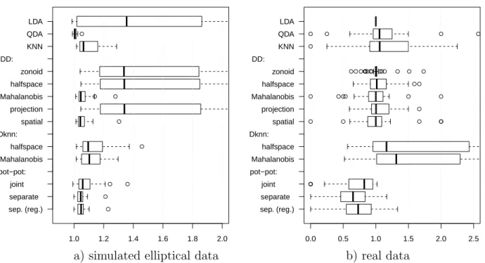
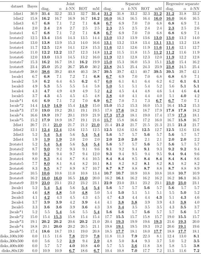
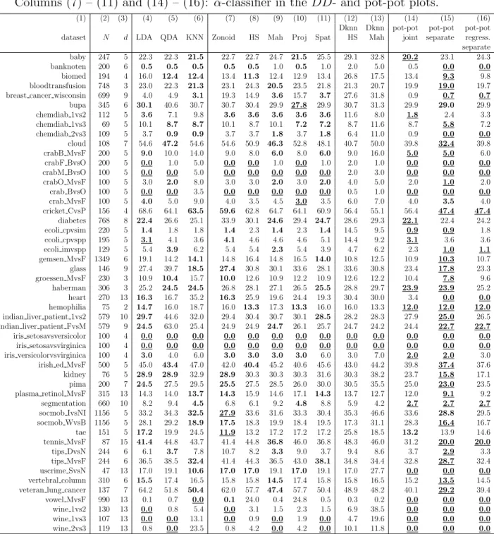
For this, either the α-procedure or the k-nearest neighbors classifier is employed. Thus the bias in kernel density estimates due to insufficiently adapted multivariate kernels is compensated by a flexible classifier on the pot-pot plot. The potentials depend on the kernel and its bandwidth used in the density estimate. We investigate several variants of bandwidth selection, including joint and separate pre-scaling and a bandwidth regression approach. The new method is applied to benchmark data from the literature, including simulated data sets as well as 50 sets of real data. It compares favorably to known classification methods such as LDA, QDA, maximal kernel density estimates, k-NN, and DD-plot classification. This chapter is based on a joint paper with Prof. Karl Mosler. The proposed method has been implemented in the R-package ddalpha. The paper has been published in the journal Statistical Papers.

In the third chapter named Depth and depth-based classification with R-package ddalpha we

describe our package ddalpha that provides an implementation for exact and approximate com-

putation of seven most reasonable and widely applied depth notions: Mahalanobis, halfspace,

zonoid, projection, spatial, simplicial and simplicial volume. The main feature of the proposed

methodology on the DD-plot is the DDα-classifier, which is an adaptation of the α-procedure

to the depth space. Except for its efficient and fast implementation, ddalpha suggests other

classification techniques that can be employed in the DD-plot: the original polynomial sepa-

rator and the depth-based k-NN-classifier. Unlike other packages, ddalpha implements various

depth functions and classifiers for multivariate and functional data under one roof. The func-

tional data are transformed into a finite dimensional basis and classified there. ddalpha is the only package that implements zonoid depth and efficient exact halfspace depth. All depths in the package are implemented for any dimension d ≥ 2. Except for the projection depth all implemented algorithms are exact, and supplemented by their approximating versions to deal with the increasing computational burden for large samples and higher dimensions. The package is expandable with user-defined custom depth methods and separators. Insights into data geometry as well as assessing the pattern recognition quality are feasible by functions for depth visualization and by built-in benchmark procedures. This chapter carries on joint work with Pavlo Mozharovskyi and Prof. Rainer Dyckerhoff. The paper has been submitted to the Journal of Statistical Software.

The fourth chapter named Depth-weighted Bayes classification introduces two procedures for supervised classification that focus on the centers of the classes and are based on data depth. The classifiers add either a depth or a depth rank term to the objective function of the Bayes classifier. The cost of misclassification of a point depends not only on its belongingness to a class but also on its centrality in this class. Classification of more central points is enforced while outliers are underweighted. The proposed objective function may also be used to evaluate the performance of other classifiers instead of the usual average misclassification rate. The usage of the depth function increases the robustness of the new procedures against big inclusions of contaminated data, which impede the Bayes classifier. At the same time smaller contaminations distort the outer depth contours only slightly and thus cause only small changes in the classification procedure. This chapter is a result of a cooperation with Ondrej Vencalek from Palacky University Olomouc.

The fifth chapter named Computation of the Oja median by bounded search suggests a new algorithm for the exact calculation of the Oja median. It modifies the algorithm of Ronkainen et al. (2003) by employing bounded regions which contain the median. The regions are built using the centered rank function. The new algorithm is faster and has lower complexity than the previous one and is able to calculate data sets of the same size and dimension. It is mainly restricted by the amount of RAM, as it needs to store all

hyperplanes. It can also be used

for an even faster approximative calculation, although it still needs the same amount of RAM

and is slower than existing approximating algorithms. The new algorithm was implemented

as a part of the R-package OjaNP. The chapter is partially based on a paper with Prof. Karl

Mosler that has been published in the book Modern Nonparametric, Robust and Multivariate

Methods: Festschrift in Honour of Hannu Oja. Some material of the chapter is taken from

our joint paper with Daniel Fischer, Jyrki M¨ ott¨ onen, Klaus Nordhausen and Daniel Vogel,

submitted to the Journal of Statistical Software.

Classification with the pot-pot plot

2.1 Introduction

Statistical classification procedures belong to the most useful and widely applied parts of statistical methodology. Problems of classification arise in many fields of application like economics, biology, medicine. In these problems objects are considered that belong to q ≥ 2 classes. Each object has d attributes and is represented by a point in d-space. A finite number of objects is observed together with their class membership, forming q training classes. Then, objects are observed whose membership is not known. The task of supervised classification consists in finding a rule by which any object with unknown membership is assigned to one of the classes.

A classical nonparametric approach to solve this task is by comparing kernel density esti- mates (KDE); see e.g. Silverman (1986). The Bayes rule indicates the class of an object x as argmax

(p

f

(x)), where p

is the prior probability of class j and f

its generating density. In KDE classification, the density f

is replaced by a proper kernel estimate ˆ f

and a new object is assigned to a class j at which its estimated potential,

φ ˆ

(x) = p

f ˆ

(x) , (2.1)

is maximum. It is well known (e.g. Devroye et al. (1996)) that KDE is Bayes consistent, that means, its expected error rate converges to the error rate of the Bayes rule for any generating densities.

As a practical procedure, KDE depends largely on the way by which the density estimates f ˆ

and the priors p

are obtained. Many variants exist, differing in the choice of the multivariate kernel and, particularly, its bandwidth matrix. Wand and Jones (1993) demonstrate that the choice of bandwidth parameters strongly influences the finite sample behavior of the KDE -classifier. With higher-dimensional data, it is computationally infeasible to optimize a full bandwidth matrix. Instead, one has to restrict on rather few bandwidth parameters.

In this chapter we modify the KDE approach by introducing a more flexible assignment

rule in place of the maximum potential rule. We transform the data to a low-dimensional

space, in which the classification is performed. Each data point x is mapped to the vector

(φ

(x), . . . , φ

(x))

in R

. The potential-potential plot, shortly pot-pot plot, consists of the transformed data of all q training classes and the transforms of any possible new data to be classified. With KDE, according to the maximum potential rule, this plot is separated into q parts,

{x ∈ R

: j = argmax

i

( ˆ φ

(x))} . (2.2)

If only two classes are considered, the pot-pot plot is a subset of R

, where the coordinates correspond to potentials regarding the two classes. Then, KDE corresponds to separating the classes by drawing the diagonal line in the pot-pot plot.

However, the pot-pot plot allows for more sophisticated classifiers. In representing the data, it reflects their proximity in terms of differences in potentials. To separate the training classes, we may apply any known classification rule to their representatives in the pot-pot plot.

Such a separating approach, being not restricted to lines of equal potential, is able to provide better adapted classifiers. Specifically, we propose to use either the k-NN-classifier or the α- procedure to be used on the plot. By the pot-pot plot procedure – once the transformation and the separator have been established – any classification step is performed in q-dimensional space.

To construct a practical classifier, we first have to determine proper kernel estimates of the potential functions for each class. In doing this, the choice of a kernel, in particular of its bandwidth parameters, is a nontrivial task. It requires the analysis and comparison of many possibilities. We evaluate them by means of the classification error they produce, using the following cross-validation procedure: Given a bandwidth matrix, one or more points are continuously excluded from the training data. The classifier is trained on the restricted data using the selected bandwidth parameter; then its performance is checked with the excluded points. The average portion of misclassified objects serves as an estimate of the classification error. Notice that a kernel bandwidth minimizing this criterion may yield estimated densities that differ significantly from the actual generating densities of the classes.

Then we search for the optimal separation in q-dimensional space of the pot-pot plot. This, in turn, allows us to keep the number of bandwidth parameters reasonably low, as well as the number of their values to be checked.

The principal achievements of this approach are:

• The possibly high dimension of original data is reduced by the pot-pot transformation so that the classification can be done on a low-dimensional space, whose dimension equals the number of classes.

• The bias in kernel density estimates due to insufficiently adapted multivariate kernels is compensated by a flexible classifier on the pot-pot plot.

1

z

denotes the transpose of z.

• In case of two classes, the proposed procedures are either always strongly consistent (if the final classifier is k-NN) or strongly consistent under a slight restriction (if the final classifier is the α-classifier).

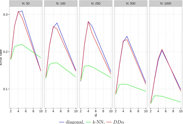
• The two procedures, as well as a variant that scales the classes separately, compare favourably with known procedures such as linear and quadratic discrimination and DD- classification based on different depths, particularly for a large choice of real data.

The chapter is structured as follows. Section 2.2 presents density-based classifiers and the Kernel Discriminant Method. Section 2.3 treats the problem of selecting a kernel bandwidth.

The pot-pot plot is discussed in Section 2.4, and the consistency of the new procedures is established in Section 2.5. Section 2.6 presents a variant of pre-scaling the data, namely separate scaling. Experiments with simulated as well as real data are reported in Section 2.7.

Section 2.8 concludes.

2.2 Classification by maximum potential estimate

Comparing kernel estimates of the densities or potentials is a widely applied approach in classification. Consider a data cloud X of points x

, . . . , x

∈ R

and assume that the cloud is generated as an independent sample from some probability density f . The potential of a given point x ∈ R

regarding the data cloud X is estimated by a kernel estimator.

Let K

(x, x

) = | det H|

K

H

(x − x

)

, H be a symmetric and positive definite bandwidth matrix, H

be a square root of its inverse, and K : R

→ [0, ∞[ be a spherical probability density function, K(z) = r(z

z), with r : [0, ∞[→ [0, ∞[ non-increasing and bounded. Then

f ˆ

(x) = 1 n

n

X

i=1

K

(x, x

) (2.3)

= 1

n

n

X

i=1

| det H|

K H

(x − x

)

is a kernel estimator of the density of x with respect to X . In particular, the Gaussian function K(z) = (2π)

exp −

z

z

will be employed below.

Let H

be an affine invariant estimate of the dispersion of X, that is,

H

= AH

A

for any A of full rank and b ∈ R

. (2.4) Then H

1 2

AX+b

= (AH

A

)

= (AH

1 2

X

)

= H

1 2

X

A

and f ˆ

(Ay + b) = 1

n

n

X

i=1

| det A|

| det H

|

K H

1 2

X

A

(Ay − Ax

)

| A|

ˆ

Hence, in this case, the potential is affine invariant, besides a constant factor | det A|

. Examples

• If H

= h

Σ ˆ

, (2.4) is satisfied; the potential is affine invariant (besides a factor).

• If H

= h

I and A is orthogonal, we obtain H

= h

I = h

AA

= AH

A

, hence (2.4); the potential is orthogonal invariant.

• If H

= h

diag(ˆ σ

, . . . , σ ˆ

) and A = diag(a

, . . . , a

), then H

= h

diag(a

σ ˆ

, . . . , a

σ ˆ

) = AH

A

; the potential is invariant regarding componentwise scaling.

The selection of the bandwidth matrices H is further discussed in Section 2.3.

Now, consider a classification problem with q training classes X

, . . . , X

, generated by densities f

, . . . , f

, respectively. Let the class X

consist of points x

, . . . , x

. The potential of a point x with respect to X

is estimated by

φ ˆ

(x) = p

f ˆ

(x) = 1 n

nj

X

i=1

K

(x, x

), (2.5)

j = 1, . . . , q. Figure 2.1 exhibits the potentials of two classes A

= {x

, x

, x

} and A

= {x

, x

}.

Figure 2.1: Potentials of two classes, {x

, x

, x

} and {x

, x

}.

The Bayes rule yields the class index of an object x as argmax

(p

f

(x)), where p

is the prior probability of class j. The potential discriminant rule mimics the Bayes rule: Estimating the prior probabilities by p

= n

/ P

k=1

n

it yields argmax

j

(p

f ˆ

(x)) = argmax

j nj

X

i=1

K

(x, x

). (2.6)

2.3 Multivariate bandwidth

The kernel bandwidth controls the range on which the potentials change with a new observa-

for both classes and apply this kernel to the data as given. This means that the kernels are spherical and treat the neighborhood of each point equally in all directions. However, the dis- tributions of the data are often not close to spherical, thus with a single-parameter spherical kernel the estimated potential differs from the real one more in some directions than in the others (Figure 2.2.a). In order to fit the kernel to the data a proper bandwidth matrix H is selected (Figure 2.2.b). This matrix H can be decomposed into two parts, one of which follows the shape of the data, and the other the width of the kernel. Then the first part may be used to transform the data, while the second is employed as a parameter of the kernel and tuned to achieve the best separation (Figure 2.2.b,c).

a) b) c)

Figure 2.2: Different ways of fitting a kernel to the data: a) applying a spherical kernel to the original data; b) applying an elliptical kernel to the original data; c) applying a spherical kernel to the transformed data.

Wand and Jones (1993) distinguish several types of bandwidth matrices to be used in (2.3) and (2.5): a spherically symmetric kernel bandwidth matrix H

= h

I with one parameter;

a matrix with d parameters H

= diag(h

, h

, ..., h

), yielding kernels that are elliptical along the coordinate axes; and an unrestricted symmetric and positive definite matrix H

having

d(d+1)

2

parameters, that produces elliptical kernels with an arbitrary orientation. With more parameters the kernels are more flexible, but require more costly tuning procedures. The data may also be transformed beforehand using their mean ¯ x and either the marginal variances ˆ

σ

or the full empirical covariance matrix ˆ Σ. These approaches are referred to as scaling and sphering. They employ the matrices C

= h

D ˆ and C

= h

Σ, respectively, where ˆ D ˆ = diag(ˆ σ

, . . . , σ ˆ

). The matrix C

is a special case of H

, and the matrix C

is a special case of H

. Each has only one tuning parameter h

and thus the same tuning complexity as H

, but fits the data much better. Clearly, the bandwidth matrix C

= h

Σ ˆ is equivalent to the bandwidth matrix H

= h

I applied to the pre-scaled data x

= ˆ Σ

1

2

(x − x). ¯

Wand and Jones (1993) show by experiments that sphering with one tuning parameter

h

shows poor results compared to the use of H

or H

matrices. Duong (2007) suggests

to employ at least a diagonal bandwidth matrix H

together with a scaling transformation,

H = ˆ Σ

H

Σ ˆ

. But, even in this simplified procedure the training time grows exponentially

with the number of tuned parameters, that is the dimension of the data.

In density estimation the diagonal bandwidth matrix H

is often chosen by a rule of thumb (H¨ ardle et al., 2004),

h

= 4

d + 2

n

σ ˆ

, (2.7)

which is based on an approximative normality assumption, and for the univariate case coincides with that of Silverman (1986). As the first factor in (2.7) is almost equal to one, the rule is further simplified to Scott’s rule (Scott, 1992), h

= n

σ ˆ

. If the covariance structure is not negligible, the generalized Scott’s rule may be used, having matrix

H

= n

Σ ˆ . (2.8)

Observe that the matrix H

is of type C

. Equivalently, after sphering the data with ˆ Σ, a bandwidth matrix of type H

is applied with h

= n

.

Here we propose procedures that employ one-parameter bandwidths combined with spher- ing transformations of the data. While this yields rather rough density estimates, the impreci- sion of the potentials is counterbalanced by a sophisticated non-linear classification procedure on the pot-pot plot. The parameters tuning procedure works as follows: The bandwidth pa- rameter is systematically varied over some range, and a value is selected that gives smallest classification error.

2.4 Pot-pot plot classification

In KDE classification a new object is assigned to the class that grants it the largest po- tential. A pot-pot plot allows for more sophisticated solutions. By this plot, the original d-dimensional data is transformed to q-dimensional objects. Thus the classification is per- formed in q-dimensional space.

E.g. for q = 2, denote the two training classes as X

= {x

, . . . , x

} and X

= {x

, . . . , x

}. Each observed item corresponds to a point in R

. The pot-pot plot Z consists of the potential values of all data w.r.t. the two classes.

Z = {z

= (z

, z

) : z

= φ

(x

), z

= φ

(x

), i = 1, ..., n + m} .

Obviously, the maximum-potential rule results in a diagonal line separating the classes in the pot-pot plot.

However, any classifier can be used instead for a more subtle separation of the classes

in the pot-pot plot. Special approaches to separate the data in the pot-pot plot are: using

k-nearest neighbors (k-NN) or linear discriminant analysis (LDA), regressing a polynomial line,

or employing the α-procedure. The α-procedure is a fast heuristic that yields a polynomial

separator; see Lange et al. (2014b). Besides k-NN, which classifies directly to q ≥ 2 classes in

the pot-pot plot, the other procedures classify to q = 2 classes only. If q > 2, several binary

classifications have to be performed, either q ‘one against all’ or q(q − 1)/2 ‘one against one’, and be aggregated by a proper majority rule.

Recall that our choice of the kernel needs a cross-validation of the single bandwidth pa- rameter h. For each particular pot-pot plot an optimal separation is found by selecting the appropriate number of neighbors for the k-NN-classifier, or the degree of the α-classifier. For the α-classifier a selection is performed in the constructed pot-pot plot, by dividing its points into several subsets, sequentially excluding one of them, training the pot-pot plot classifier using the others and estimating the classification error in the excluded subset. For the k-NN- classifier an optimization procedure is used that calculates the distances from each point to the others, sorts the distances and estimates the classification error for each value of k. The flexibility of the final classifier compensates for the relative rigidity of the kernel choice.

Our procedure bears an analogy to DD-classification, as it was introduced by Li et al.

(2012). There, for each pair of classes, the original data are mapped to a two-dimensional depth-depth (DD) plot and classified there. A function x 7→ D

(x|X) is used that indicates how central a point x is situated in a set X of data or, more general, in the probability distribution of a random vector X in R

. The upper level sets of D

(·|X) are regarded as

‘central regions’ of the distribution. D

(·|X) is called a depth function if its level sets are

• closed and bounded,

• affine equivariant, that is, if X is transformed to AX + b with some regular matrix A ∈ R

and b ∈ R

, then the level sets are transformed in the same way.

Clearly, a depth function is affine invariant; D

(x|X) does not change if both x and X are subjected to the same affine transformation. For surveys on depth functions and their properties, see e.g. Zuo and Serfling (2000), Serfling (2006), and Mosler (2013).

More generally, in DD-classification, the depth of all data points is determined with respect to each of the q classes, and a data point is represented in a q-variate DD-plot by the vector of its depths. Classification is done on the DD-plot, where different separators can be employed. In Li et al. (2012) a polynomial line is constructed, while Lange et al. (2014b) use the α-procedure and Vencalek (2014) suggests to apply k-NN in the depth space. Similar to the polynomial separator of Li et al. (2012), the α-procedure results in a polynomial separation, but is much faster and produces more stable results. Therefore we focus on the α-classifier in this chapter.

Note that Fraiman and Meloche (1999) mention a density estimate ˆ f

(x) as a ‘likelihood

depth’. Of course this ‘depth’ does not satisfy the usual depth postulates. Principally, a depth

relates the data to a ‘center’ or ‘median’, where it is maximal; a ‘local depth’ does the same

regarding several centers. Paindaveine and Van Bever (2013) provide a local depth concept

that bears a connection with local centers. Different from this, a density estimate measures

at a given point how much mass is located around it; it is of a local nature, but not related

to any local centers. This fundamental difference has consequences in the use of these notions

as descriptive tools as well as in their statistical properties, e.g. regarding consistency of the

resulting classifiers; see also Paindaveine and Van Bever (2015). Appendix at the end of the

thesis contains an overview of local depths.

Maximum-depth classification with the ‘likelihood depth’ (being weighted with prior prob- abilities) is the same as KDE. Cuevas et al. (2007) propose an extension of this notion to functional data, the h-depth that is calculated as ˆ D

(x) =

P

i=1

K

, where m is a distance. The h-depth is used in Cuesta-Albertos et al. (2016), among several genuine depth approaches, in a generalized DD-plot to classify functional data. However, the DD

classifier with h-depth applies equal spherical kernels to both classes, with the same parameter h. The authors also do not discuss about the selection of h, while Cuevas et al. (2007) proposed keeping it constant for the functional setup. Our contribution differs in many respects from the latter one: (1) We use Gaussian kernels with data dependent covariance structure and optimize their bandwidth parameters. (2) The kernel is selected either simultaneously or separately for each class. (3) When q = 2, in case of separate sphering, a regression between the two bandwidths is proposed, that allows to restrict the optimization to just one bandwidth parameter (see sec.

2.6). (4) Strong consistency of the procedure is demonstrated (see the next Section). (5) The procedure is compared with known classification procedures on a large number of real data sets (see Section 2.7).

2.5 Bayes consistency

We advocate the pot-pot procedure as a data-analytic tool to classify data of unknown origin, generally being non-normal, asymmetric and multi-modal. Nevertheless, it is of more than theoretical interest, how the pot-pot procedure behaves when the sample size goes to infinity.

Regarded as a statistical regression approach, Bayes consistency is a desirable property of the procedure.

We consider the case q = 2. The data are seen as realizations of a random vector (X , Y ) ∈ R

× {1, 2}, that has probability distribution P . A classifier is any function g : R

→ {1, 2}.

Notate p

(x) = P (Y = j|X = x). The Bayes classifier g

is given by g

(x) = 2 if p

(x) >

p

(x) and g

(x) = 1 otherwise. Its probability of misclassification, P (g

(X) 6= Y ) is the best achievable risk, which is named the Bayes risk.

We assume that the distributions of (X , 1) and (X, 2) are continuous. Let the potentials be estimated by a continuous regular kernel (see Definition 10.1 in Devroye et al. (1996)), like a Gaussian kernel, and let (h

) be a sequence of univariate bandwidths satisfying

h

→ 0 and nh

→ ∞ . (2.9)

It is well-known (see Theorem 10.1 in Devroye et al. (1996)) that then the maximum potential rule is strongly Bayes-consistent, that is, its error probability almost surely approaches the Bayes risk for any continuous distribution of the data. The question remains, whether the proposed procedures operating on the pot-pot plot attain this risk asymptotically.

We present two theorems about the Bayes consistency of the two variants of the pot-pot

classifier.

Theorem 2.1 (k-N N ) Assume that (X, 1) and (X, 2) have continuous distributions. Then the pot-pot procedure is strongly Bayes consistent if the separation on the pot-pot plot is per- formed by k-nearest neighbor classification with k

→ ∞ and k

/n → 0.

Proof: Let us first define a sequence of pot-pot classifiers that satisfies (2.9). We start with two training classes of sizes n

and n

, set n

= n

+n

, and determine a proper bandwidth h

by cross-validation as described above. Then, let n

→ ∞ and n

→ ∞, n = n

+ n

. For n > n

we restrict the search for h

to the interval

h

h

· n

, h

· n

i ,

with some 0 < ≤ δ < 1. It follows that h

→ 0 and nh

→ ∞ as n goes to infinity, which yields the a.s. strong Bayes consistency of the maximum potential rule. The maximum potential rule corresponds to the diagonal of the pot-pot plot. This separator almost surely asymptotically attains the Bayes risk.

We have still to demonstrate that the k-nearest neighbor procedure applied to the trans- formed data on the pot-pot plot yields the same asymptotic risk. Under k

→ ∞ and k

/n → 0, the k-N N procedure on the pot-pot plot is strongly Bayes consistent if either φ

(X) or φ

(X ) is continuously distributed in R

; see Theorem 11.1 and page 190 in Devroye et al. (1996).

But the latter follows from the continuity of the regular kernel. Obviously, the Bayes risk of classifying the transformed data is the same as that of classifying the original data. It follows that for any distribution of the original data the pot-pot procedure achieves the Bayes risk

almost surely asymptotically.

Theorem 2.2 (α-procedure) Assume that (X, 1) and (X , 2) have continuous distributions and that

P (p

(X) = p

(X )) = 0 . (2.10)

Then the pot-pot procedure is strongly Bayes consistent if the separation on the pot-pot plot is performed by the α-procedure.

Proof: As in the preceding proof, the maximum potential rule corresponds to the diagonal of the pot-pot plot, and this separator almost surely asymptotically attains the Bayes risk.

Consider the sign of the difference between the two (estimated) potentials. If the sample size goes to infinity the number of ’wrong’ signs goes to zero. By assumption (2.10) also the number of ties (corresponding to points on the diagonal) goes to zero. By definition, the α-procedure in its first step considers all pairs of features, the original z

and z

and possibly polynomials of them up to some pre-given degree. Then for each pair a separating line is determined that minimizes the empirical risk; see Lange et al. (2014b). Thus, once the differences of the potentials have the correct sign, the α-procedure will produce the diagonal of the (z

, z

)-plane (or a line that separates the same points) in its very first step.

Compared to these results, the Bayes consistency of depth-depth (DD) plot procedures

symmetric distributions; see Li et al. (2012) and Lange et al. (2014b). The reason is that depth functions fit primarily to unimodal distributions. Under unimodal ellipticity, since a depth function is affine invariant, its level sets are ellipsoids that correspond to density level sets, and the depth is a monotone function of the density.

Note that the distributions of the two training classes, after having been transformed by the

‘sphering transformation’, can be still far away from being spherical. This happens particularly often with real data. It is well known that with a single parameter the multidimensional poten- tials are often poorly estimated by their kernel estimates. Then the best separator may differ considerably from the diagonal of the pot-pot plot as our results will demonstrate, see Figure 2.3. The final classification on the plot compensates the insufficient estimate by searching for the best separator on the plot.

● ●●

●

●

●

●

●

●

●

●

●

●

●

●

●

●

●

●

●

●

●

●

●

●●

●

●

●

●

●

●●

●

●

●

●

● ●

●●●●●

●

●

●●

●

●

●

●

●

●

●

●

●

●●

●

●

●

●

●

●

●

●

●

●

●●

●

●

●

●

●

●

●

●

● ●

●

● ●

●

●

●

0e+00 2e−08 4e−08 6e−08 8e−08 1e−07

0e+002e−084e−086e−088e−081e−07

●

●

●

●

●

● ● ●

● ●

●

● ●●

●

●

●

●

●

●

●

●

●

●

●

●

●

●

● ●

● ●

● ●

●

●

●

●

●

● ● ●

●

●

●

●

●

●

● ●

●

●

● ●

●

●

● ●

●

●

●

●

●

● ●●

●

● ●

●

●

●

●

●

●

●

●

●

● ●

●

●

●

●

● ●

●

●

●

● ●

●

● ●

●

●

●

●

● ●

●

●

●

●●

●

●

●

●

●

●

●

●

● ●

●

● ● ●

●

●

● ●

●

●

●

●

●

●

● ●

●

●

● ●

●

●

●

●

●

●

●

●

● ●

●

● ●

●

● ●●

●

●

●

●

● ●

●

●

● ●●

●

●

●

● ●

●

● ●

●

●●

● ●

● ● ●

●

● ●

●

●

●

●

● ●

●

●

●

●

● ●

● ●

●

●

●

● ●

●

●

● ●

●

●

● ●

● ● ●

●

●

● ●

●

● ●

●

● ●● ●

● ●

●

●

●

● ●

● ●

●

●

● ●

●

●

●

●

●

●

● ● ●

●

0.0 0.1 0.2 0.3

0.00.10.20.3

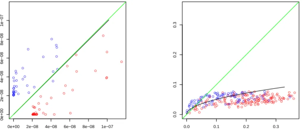
Figure 2.3: Examples of α-separation in the pot-pot plot. In the left panel (data set ‘tennis’) the α-classifier coincides with the diagonal, while in the right panel (data set ‘baby’) it provides a completely different separation. Bandwidth parameters are selected according to best performance of the α-classifier.

2.6 Scaling the data

In Section 2.3 we have shown that it is convenient to divide the bandwidth matrix into two parts, one of which is used to scale the data, and the other one to tune the width of a spherical kernel. The two classes may be scaled jointly or separately, before proper bandwidth parameters are tuned. Note that Aizerman et al. (1970) do not scale the data and use the same kernel for both classes.

KDE naturally estimates the densities individually for each class and tunes the bandwidth

matrices separately. On the other hand, SVM scales the classes jointly (Chang and Lin, 2011),

either dividing each attribute by its standard deviation, or scaling it to [0; 1].

In what follows we consider two approaches: joint and separate scaling. With joint scaling the data is sphered using a proper estimate ˆ Σ of the covariance matrix of the merged classes;

then a spherical kernel of type H

is applied. This results in potentials φ

(x) = p

f ˆ

(x) = p

1

n

nj

X

i=1

K

(x − x

) ,

where an estimate ˆ Σ of the covariance matrix has to be calculated and one scalar parameter h

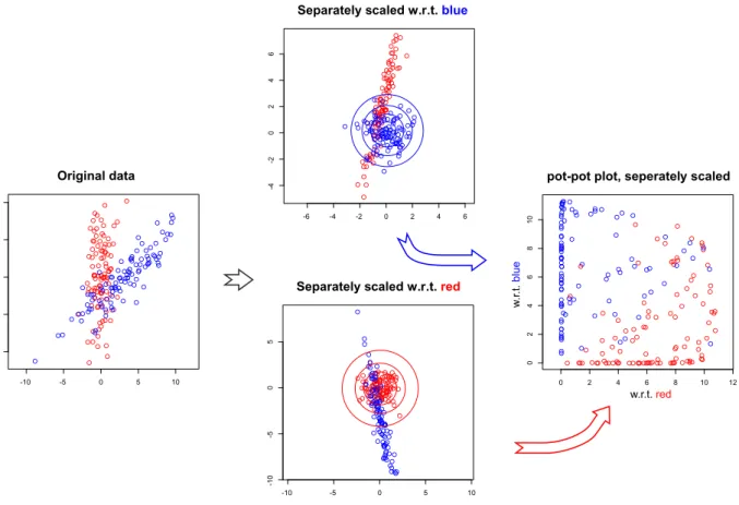
has to be tuned. (Note that ˆ Σ is not necessarily the empirical covariance matrix; in particular, some more robust estimate may be used.) The scaling procedure and the obtained pot-pot plot are illustrated in Fig. 2.4. Obviously, as the classes differ, the result of joint scaling is far away from being spherical and the spherical kernel does not fit the two distributions well. However, these kernels work well when the classes’ overlap is small; in this case the separation is no big task.

An alternative is separate scaling. It results in potentials φ

(x) = p

f ˆ

(x) = p

1

n

nj

X

i=1

K

jΣˆj

(x − x

) .

With separate scaling the two kernels are built with different bandwidth matrices H

= C

= h

Σ ˆ

to fit the form of each class. We need estimates of two covariance matrices and have two parameters, h

and h

, to tune. Figure 2.5 illustrates the approach. It is clearly seen that many points receive much less potential with respect to the opposite class.

In case of heavy-tailed data, robustness is achieved by applying the Minimum Covariance Determinant (MCD) or the Minimum Volume Ellipsoid (MVE) estimates to transform the data. Note, that in some cases the problem may occur, that the covariance matrix is singular, e.g. if the dimension is higher than the number of points. In this case one may use a proper pseudoinverse.

As tuning the parameters comes at high computational costs, we try to simplify the tuning in the case of separate scaling. Either we use the same parameter, h

= h

for both classes or we establish some relationship between the two parameters, h

= g(h

) where g is a function of the first bandwidth. After a proper function g is found only one parameter must be tuned.

In our experiments (sec. 7), we observe a relationship between the bandwidth parame-

ters that provide the smallest error rates. For the real data sets we see that, with separate

scaling, close to smallest classification errors are usually achieved on a straight line in the

(log

h

, log

h

)-plane (see Fig. 2.7 and the description there). We profit from this observa-

tion and spare the effort of separately tuning the two parameters. Note that the line is not

always the main diagonal. We propose to regress one parameter on the other, evaluating the

error at a few pairs (log

h

, log

h

) and using them as sampling points. Specifically, we cal-

culate the error at five sets of five points, with the five-point sets being taken orthogonally to

the main diagonal of the plot; cf. Figures 2.6 and 2.7. Then the minimal error is found in each