Shapes and Dynamics of Blood Cells in Poiseuille and Shear Flows

Poiseuille and Shear Flows

Inaugural-Dissertation

zur

Erlangung des Doktorgrades

der Mathematisch-Naturwissenschaftlichen Fakult¨at der Universit¨at zu K ¨oln

vorgelegt von

Johannes Mauer aus Koblenz

J ¨ulich

2016

Berichterstatter (Gutachter):

Prof. Dr. Gerhard Gompper Prof. Dr. Andreas Schadschneider

Tag der m ¨undlichen Pr ¨ufung: 15. April 2016

Kurzzusammenfassung

Die Dynamik, Form, Verformung und Ausrichtung roter Blutzellen in der Mikrozirkulation beeinflussen Rheologie, Fließwiderstand und Transporteigenschaften des Blutes. Dies f ¨uhrt zu wichtigen Zusammenh¨angen der zellul¨aren und Kontinuums-Skalen. Des Weiteren ist die Dynamik roter Blutzellen, die verschiedenen Str ¨omungen und Gef¨aßgeometrien unter- liegen, relevant f ¨ur sowohl Grundlagenforschung als auch biomedizinische Anwendungen (z.B. Medikamentenzuf ¨uhrung).

In dieser Arbeit wird das Verhalten roter Blutzellen f ¨ur verschiedene Str ¨omungen mittels Computersimulationen untersucht. Wir benutzen eine Kombination zweier mesoskopischer teilchenbasierter Simulationstechniken, Dissipative Particle Dynamics und Smoothed Dis- sipative Particle Dynamics. Wir konzentrieren uns auf die mikrokapillarische Skala von einigen µm. Auf dieser Skala kann Blut nicht auf der Kontinuumsskala betrachtet, sondern muss auf der zellul¨aren Skala untersucht werden. Die Verkn ¨upfung zwischen zellul¨arer Be- wegung und Blut-Rheologie wird untersucht.

Rote Blutzellen werden als viskoelastische Objekte modelliert, die mit einer viskosen fl ¨us- sigen Umgebung wechselwirken. Die Membraneigenschaften, wie Biegesteifigkeit oder Scher- festigkeit, sind so gew¨ahlt, dass sie experimentellen Werten entsprechen. Des Weiteren wer- den thermische Fluktuationen mittels Zufallskr¨aften betrachtet.

Analysen, die Lichtstreuungsmessungen entsprechen, werden durchgef ¨uhrt, um mit Experi- menten zu vergleichen und nahezulegen, f ¨ur welche Situationen diese Methode geeignet ist.

Statische Lichtstreuung von roten Blutzellen charakterisiert deren Form und erlaubt Vergle- iche mit Objekten wie Kugeln oder Zylindern, deren Lichtstreuungssignale analytisch l ¨osbar sind, im Gegensatz zu denen roter Blutzellen. Dynamische Lichtstreuung roter Blutzellen wird hinsichtlich seiner Eignung, Bewegungen, Verformungen und Membranfluktuationen nachzuweisen und zu analysieren, untersucht. Analysen zur dynamischen Lichtstreuung werden sowohl f ¨ur diffundierende als auch fließende Zellen durchgef ¨uhrt. Streusignale h¨angen von den Zelleigenschaften ab und erlauben daher, verschiedene Zellen voneinander abzugrenzen. Die Streuung diffundierender Zellen l¨asst mittels des effektiven Diffusionsko- effizienten R ¨uckschl ¨usse auf ihre Biegesteifigkeit zu. Die Streuung fließender Zellen l¨asst mittels der Streuamplitudenkorrelation R ¨uckschl ¨usse auf die Scherrate zu.

Im Fluss weist eine rote Blutzelle verschiedene Formen und dynamische Zust¨ande auf, ab- h¨angig von Bedingungen wie eingeschr¨ankter Geometrie, physiologischen/pathologischen Zust¨anden und Zellalter. In dieser Arbeit werden zwei wesentliche Str ¨omungen untersucht:

einfacher Scherfluss und Fluss durch eine zylindrische R ¨ohre.

Einfacher Scherfluss als eine grundlegende Str ¨omung ist Teil jeder komplexeren Str ¨omung.

Das Geschwindigkeitsprofil ist linear und die Scherspannung ist homogen. In einfachem Scherfluss finden wir eine Abfolge verschiedener Zellformen, wenn die Scherrate erh ¨oht wird. Mit steigender Scherrate finden wir rollende Zellen in Schalenform, Trilobe- und

v

Quadrulobe-Formen. Dies stimmt mit aktuellen Experimenten ¨uberein. Des Weiteren wird der Einfluss der anf¨anglichen Ausrichtung auf die Dynamik untersucht. Um Verdr¨angungs- und kollektive Effekte zu untersuchen, werden Systeme mit h ¨oherem H¨amatokrit aufge- setzt.

Die Str ¨omung durch eine R ¨ohre dient als idealisiertes Modell f ¨ur die Str ¨omung durch an- n¨ahernd zylinderf ¨ormige Mikrogef¨aße. Ohne Zelle liegt ein parabolisches Geschwindigkeit- sprofil vor. Eine einzelne rote Blutzelle wird in der R ¨ohre platziert und einem Poiseuille- Profil ausgesetzt. Bei der Rohr-Str ¨omung finden wir verschiedene Zellformen und -dynamiken, abh¨angig von der Einschr¨ankung durch Geometrie (hier der Rohrdurchmesser), Scherrate und Zelleigenschaften. F ¨ur enge R ¨ohren und hohe Scherraten finden wir Fallschirm-f ¨ormige Zellen. Obwohl nicht perfekt symmetrisch, sind sie dem Flussprofil angepasst und be- halten eine station¨are Form und Ausrichtung. F ¨ur weite R ¨ohren und niedrige Scherraten finden wir taumelnde Slipper-Formen, die sich drehen und ihre Form moderat ¨andern.

F ¨ur weite R ¨ohren und hohe Scherraten finden wir Slippers mit sogenannter Panzerketten- Membranrotation, die ihren Anstellwinkel leicht oszillieren und periodisch ihre Form stark

¨andern. F ¨ur die niedrigsten Scherraten finden wir Zellen, die eine Schl¨angelbewegung ausf ¨uhren. Aufgrund der Zelleigenschaften und sich daraus ergebender Verformungen un- terscheiden sich alle Formen von bisherigen Beschreibungen in der Literatur, wie z.B. sta- tion¨are Panzerketten-Membranrotation oder symmetrische Fallschirmformen. Wir f ¨uhren Phasendiagramme ein, um die Parameterbereiche verschiedener Formen und Dynamiken zu identifizieren. Ver¨andert man die Zelleigenschaften, ¨andern sich auch die Grenzen dieser Bereiche in den Phasendiagrammen.

In beiden Str ¨omungstypen sind sowohl der Viskosit¨atskontrast als auch die Wahl der span-

nungsfreien Form wichtig. Bei in vitro Experimenten war die Viskosit¨at des L ¨osungsmittels

bisher oft h ¨oher als die des Cytosols, was zu anderen Bewegungsformen f ¨uhrt, wie z.B. sta-

tion¨are Panzerketten-Membranrotation. Die spannungsfreie Form einer roten Blutzelle, die

den Zustand bei verschwindender Scherbelastung darstellt, ist noch umstritten, und Com-

putersimulationen erm ¨oglichen direkte Vergleiche m ¨oglicher Kandidaten bei ansonsten gle-

ichen Str ¨omungsbedingungen.

Abstract

The dynamics, shape, deformation, and orientation of red blood cells in microcirculation affect the rheology, flow resistance and transport properties of whole blood. This leads to important correlations of cellular and continuum scales. Furthermore, the dynamics of RBCs subject to different flow conditions and vessel geometries is relevant for both fundamental research and biomedical applications (e.g drug delivery).

In this thesis, the behaviour of RBCs is investigated for different flow conditions via com- puter simulations. We use a combination of two mesoscopic particle-based simulation tech- niques, dissipative particle dynamics and smoothed dissipative particle dynamics. We focus on the microcapillary scale of several µm. At this scale, blood cannot be considered at the continuum but has to be studied at the cellular level. The connection between cellular mo- tion and overall blood rheology will be investigated.

Red blood cells are modelled as viscoelastic objects interacting hydrodynamically with a vis- cous fluid environment. The properties of the membrane, such as resistance against bending or shearing, are set to correspond to experimental values. Furthermore, thermal fluctuations are considered via random forces.

Analyses corresponding to light scattering measurements are performed in order to com- pare to experiments and suggest for which situations this method is suitable. Static light scattering by red blood cells characterises their shape and allows comparison to objects such as spheres or cylinders, whose scattering signals have analytical solutions, in contrast to those of red blood cells. Dynamic light scattering by red blood cells is studied concerning its suitability to detect and analyse motion, deformation and membrane fluctuations. Dynamic light scattering analysis is performed for both diffusing and flowing cells. We find that scat- tering signals depend on various cell properties, thus allowing to distinguish different cells.

The scattering of diffusing cells allows to draw conclusions on their bending rigidity via the effective diffusion coefficient. The scattering of flowing cells allows to draw conclusions on the shear rate via the scattering amplitude correlation.

In flow, a RBC shows different shapes and dynamic states, depending on conditions such as confinement, physiological/pathological state and cell age. Here, two essential flow condi- tions are studied: simple shear flow and tube flow.

Simple shear flow as a basic flow condition is part of any more complex flow. The velocity profile is linear and shear stress is homogeneous. In simple shear flow, we find a sequence of different cell shapes by increasing the shear rate. With increasing shear rate, we find rolling cells with cup shapes, trilobe shapes and quadrulobe shapes. This agrees with recent exper- iments. Furthermore, the impact of the initial orientation on the dynamics is studied. To study crowding and collective effects, systems with higher haematocrit are set up.

Tube flow is an idealised model for the flow through cylindric microvessels. Without cell, a parabolic flow profile prevails. A single red blood cell is placed into the tube and subject to

vii

a Poiseuille profile. In tube flow, we find different cell shapes and dynamics depending on confinement, shear rate and cell properties. For strong confinements and high shear rates, we find parachute-like shapes. Although not perfectly symmetric, they are adjusted to the flow profile and maintain a stationary shape and orientation. For weak confinements and low shear rates, we find tumbling slippers that rotate and moderately change their shape.

For weak confinements and high shear rates, we find tank-treading slippers that oscillate in a limited range of inclination angles and strongly change their shape. For the lowest shear rates, we find cells performing a snaking motion. Due to cell properties and resultant defor- mations, all shapes differ from hitherto descriptions, such as steady tank-treading or sym- metric parachutes. We introduce phase diagrams to identify flow regimes for the different shapes and dynamics. Changing cell properties, the regime borders in the phase diagrams change.

In both flow types, both the viscosity contrast and the choice of stress-free shape are impor-

tant. For in vitro experiments, the solvent viscosity has often been higher than the cytosol

viscosity, leading to a different pattern of dynamics, such as steady tank-treading. The stress-

free state of a RBC, which is the state at zero shear stress, is still controversial, and computer

simulations enable direct comparisons of possible candidates in equivalent flow conditions.

Contents

List of Figures xiii

1 Introduction 1

1.1 Blood as a Cell Suspension . . . . 1

1.1.1 Red Blood Cells . . . . 1

1.1.2 White Blood Cells . . . . 3

1.1.3 Platelets . . . . 4

1.2 Physical Aspects of Blood Cells and Blood Flow . . . . 4

1.3 Physical Aspects of the Cardiovascular System . . . . 5

1.4 Models for Blood-Related Phenomena . . . . 6

1.4.1 Haemorheology . . . . 6

1.4.2 Haemolysis . . . . 8

1.4.3 Haemodynamic Quantities . . . . 9

1.5 Thermodynamics of Lipid Membranes . . . . 10

1.5.1 General Considerations . . . . 10

1.5.2 Elasticity and Curvature . . . . 12

1.5.3 Response Functions of a Membrane . . . . 14

1.5.4 Shapes and Deformations of Vesicles . . . . 14

1.6 Blood Flow: Previous Numerical Approaches and Results . . . . 15

2 Numerical Methods 19 2.1 Simulation Framework . . . . 19

2.1.1 Smoothed Particle Hydrodynamics . . . . 19

2.1.2 Dissipative Particle Dynamics . . . . 21

2.1.3 Smoothed Dissipative Particle Dynamics . . . . 22

2.1.4 Integration of Equations of Motion . . . . 23

2.2 Present RBC Models . . . . 23

2.2.1 Vesicle Model . . . . 24

2.2.2 Hyperelastic Model . . . . 25

2.2.3 Combined Immersed Boundary LB & FEM . . . . 26

2.2.4 Multiscale Model . . . . 28

2.3 Red Blood Cell Model of this Thesis . . . . 30

2.3.1 Membrane Triangulation . . . . 31

2.3.2 Membrane Potentials . . . . 31

2.4 Choices about the Rheological Properties of RBCs . . . . 33

2.5 Simulation Units of Measurement . . . . 35

ix

2.6 Boundary Conditions in Flow . . . . 35

2.6.1 Impermeability of Membranes and Walls . . . . 35

2.6.2 No-Slip Boundary Conditions and Adaptive Shear Force . . . . 36

3 Light Scattering by a RBC 39 3.1 Introduction . . . . 39

3.2 Characteristic Quantities . . . . 40

3.2.1 Form Factor . . . . 41

3.2.2 Structure Factor . . . . 41

3.2.3 Dynamic Scattering Function . . . . 42

3.3 Light Scattering by Simple Objects . . . . 43

3.3.1 Light Scattering by Spheres . . . . 43

3.3.2 Light Scattering by Cylinders . . . . 45

3.4 Light Scattering by Red Blood Cells . . . . 46

3.4.1 Introduction . . . . 46

3.4.2 Index of Refraction of Blood and Choice of Wavelength . . . . 47

3.4.3 Static Light Scattering by a RBC . . . . 48

3.4.4 Dynamic Light Scattering by a Diffusing RBC . . . . 50

3.4.5 Diffusion Coefficient from Hydropro . . . . 55

3.4.6 Multiple Scattering . . . . 56

3.4.7 Red Blood Cells in Shear Flow . . . . 56

3.5 Comparison with Polymers in Shear Flow . . . . 70

3.6 Conclusion . . . . 70

4 Dynamics of a RBC in Simple Shear Flow 73 4.1 Introduction . . . . 73

4.2 Models & Methods . . . . 74

4.2.1 Numerical Method . . . . 74

4.2.2 Measured Quantities . . . . 74

4.2.3 Single Cell in a Couette-Flow Setup with Walls . . . . 75

4.2.4 Multiple Cells in Shear Flow . . . . 75

4.3 Results . . . . 76

4.3.1 Single Cell in Couette-Flow Setup with walls . . . . 76

4.3.2 Multiple Cells in Shear Flow . . . . 84

4.4 Conclusion . . . . 96

5 Dynamics of a RBC in Tube Flow 99 5.1 Introduction . . . . 99

5.2 Models & Methods . . . . 100

5.2.1 Numerical interaction model . . . . 100

5.2.2 Simulated Scenario . . . . 100

5.2.3 Simulation Parameters and Scaling Equations . . . . 101

5.2.4 Red Blood Cell Model . . . . 101

5.2.5 Vessel Model . . . . 102

5.3 Distinguishing Different Shapes and Dynamics . . . . 102

5.4 Domains of Shapes and Dynamics . . . . 105

5.4.1 Phase Diagram . . . . 105

5.4.2 Representative Examples . . . . 106

5.5 Comparative Parameter Set-Ups . . . . 112

5.5.1 Viscosity Contrast of One . . . . 112

5.5.2 Viscosity Contrast of Three . . . . 113

5.5.3 Less Deformable . . . . 114

5.5.4 Spontaneous Curvature . . . . 115

5.6 A Closer Look at the Transition near the Border . . . . 116

5.7 Conclusion . . . . 117

6 Conclusion and Outlook 119

7 Thanks & Acknowledgements 123

Bibliography 125

List of Figures

1.1 Erythropoiesis . . . . 3

1.2 Whole Blood . . . . 5

1.3 Sickle Cell Anaemia . . . . 5

1.4 Viscosity as a Function of Vessel Diameter . . . . 7

1.5 Viscosity as a Function of Shear Rate . . . . 8

1.6 Lipid, Head Group and Tail Structure . . . . 10

1.7 Lipid Bilayer . . . . 11

1.8 Lipid Bilayer Embedding Proteins . . . . 11

1.9 Lipid Melting . . . . 12

1.10 RBC Membrane Composition . . . . 13

1.11 Temperature-Induced Endocytosis . . . . 15

1.12 RBC Aspirated in a Micropipette . . . . 16

1.13 Velocity Profiles for Different Haematocrit . . . . 17

2.1 IBM: membrane mesh and fluid grid . . . . 28

2.2 Multiscale Model by Peng . . . . 29

2.3 Triangulated RBC . . . . 31

2.4 Stress-Free Shapes . . . . 34

2.5 Erythroblasts . . . . 34

2.6 Viscosity Contrast . . . . 35

2.7 Simple Shear Velocity Profile . . . . 36

2.8 Sphere of Interaction . . . . 37

3.1 Light Scattering: Experimental Setup . . . . 40

3.2 Form Factor of a Sphere . . . . 43

3.3 D

(q) of a Sphere . . . . 44

3.4 Form Factor of a Cylinder; Axial ~ q . . . . 45

3.5 Form Factor of a Cylinder; Lateral ~ q . . . . 46

3.6 Light Scattering: RBC Alignment . . . . 48

3.7 Form Factor of a RBC; Different ~ q . . . . 49

3.8 Scattering Amplitude of a RBC . . . . 49

3.9 Time Averaged Intensity of a RBC . . . . 50

3.10 Intermediate Scattering Function of a RBC with κ

= 10k

T and Different q . 52 3.11 Intermediate Scattering Function of a RBC for q = 0.5/µm and Different κ

. 52 3.12 D

(q) of a RBC . . . . 53

3.13 D

(q): Different Simulations . . . . 54

xiii

3.14 D

(q) of a RBC with N

= 500 . . . . 55

3.15 DLS in Shear Setup . . . . 58

3.16 Correlation Functions S(q, t) for Different Shear Rates; Flow Direction . . . . 62

3.17 Correlation Functions S(q, t) for Different Shear Rates; Vorticity Direction . . 63

3.18 Correlation Functions S(q, t) for Different Shear Rates; Gradient Direction . . 64

3.19 Average Intensity in Flow Direction . . . . 65

3.20 Average Intensity in Vorticity Direction . . . . 66

3.21 Average Intensity in Gradient Direction . . . . 66

3.22 Correlation Decay Time in Flow Direction . . . . 67

3.23 Correlation Decay Time in Vorticity Direction . . . . 67

3.24 Correlation Decay Time in Gradient Direction . . . . 68

3.25 Correlation Decay Frequency in Flow Direction . . . . 68

3.26 Correlation Decay Frequency in Vorticity Direction . . . . 69

3.27 Correlation Decay Frequency in Gradient Direction . . . . 69

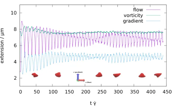
4.1 Simple Shear Flow Setup . . . . 75

4.2 Cell Extensions at γ ˙ = 57s

. . . . 77

4.3 Cell Extensions at γ ˙ = 573s

. . . . 78

4.4 Quadrulobe at γ ˙ = 2005s

. . . . 78

4.5 Orientation Angle of Initially Upright Cells . . . . 79

4.6 Membrane and Shape Motion at γ ˙ = 57s

. . . . 80

4.7 Membrane and Shape Motion at γ ˙ = 286s

. . . . 80

4.8 Orientation Angle at γ ˙ = 57s

. . . . 81

4.9 Asphericity at Shear Rates 57s

and 2005s

. . . . 81

4.10 Asphericity at Shear Rates 286s

and 573s

. . . . 82

4.11 Extensions of Cells with Different Internal Viscosity . . . . 83

4.12 Aspect Ratio of Cells with Different Internal Viscosity . . . . 84

4.13 Histogram of Eigenvalues . . . . 85

4.14 Histogram of Smallest Eigenvalue . . . . 85

4.15 Histogram of the Cell Extensions in Different Directions . . . . 86

4.16 Histogram of the Cell Extensions in Flow Direction . . . . 87

4.17 Histogram of the Acylindricity . . . . 87

4.18 Histogram of the Angle in Flow Direction (Ensemble) . . . . 88

4.19 Histogram of the Angle in Flow Direction (Single Cell) . . . . 89

4.20 Histogram of the Angle in Gradient Direction (Ensemble) . . . . 89

4.21 Histogram of the Angle in Gradient Direction (Single Cell) . . . . 90

4.22 Asphericity at Different Shear Rates . . . . 91

4.23 Asphericity at Comparable Shear Rates . . . . 91

4.24 Shear Thinning of RBC Suspension . . . . 93

4.25 Extension in Flow Direction at γ ˙ = 2000s

. . . . 93

4.26 Extension in Gradient Direction at γ ˙ = 2000s

. . . . 94

4.27 Extension in Vorticity Direction at γ ˙ = 2000s

. . . . 94

4.28 Extension in Flow Direction Phase Diagram . . . . 95

4.29 Extension in Gradient Direction Phase Diagram . . . . 95

4.30 Extension in Vorticity Direction Phase Diagram . . . . 96

5.1 Tube Flow Setup . . . . 100

5.2 Angle to the Flow Direction; Phase Diagram . . . . 103

5.3 Variation in the Angle to the Flow Direction; Phase Diagram . . . . 103

5.4 Distance to the Centre Line; Phase Diagram . . . . 104

5.5 Asphericity; Phase Diagram . . . . 104

5.6 Bending Energy; Phase Diagram . . . . 105

5.8 Phase Diagram for a Viscosity Contrast of Five . . . . 105

5.9 Angle to the Flow Direction; Representative Shapes . . . . 108

5.10 Distance to the Centre Line; Representative Shapes . . . . 108

5.11 Asphericity; Representative Shapes . . . . 108

5.12 Histogram of Angles; Representative Shapes . . . . 109

5.13 Orientation Dynamics of a Tumbling Slipper . . . . 109

5.7 Four Different Shapes/Dynamics Found in Tube Flow . . . . 111

5.14 Phase Diagram for a Viscosity Contrast of One . . . . 113

5.15 Phase Diagram for a Viscosity Contrast of Three . . . . 114

5.16 Phase Diagram for a Less Deformable Cell . . . . 115

5.17 Phase Diagram for a Cell with Spontaneous Curvature . . . . 115

Introduction

1.1 Blood as a Cell Suspension

Blood is a suspension of red and white blood cells, platelets and plasma. The latter makes up about 55% of blood volume and contains mostly water and dissolved proteins, electrolytes and smaller constituents such as neurotransmitters and hormones. Blood transports nutri- ents, metabolic waste products and oxygen to muscles and organs in living organisms [106].

The shape of red blood cells (RBCs) is intimately coupled to the ambient plasma, leading to a variety of RBC morphologies in the blood circulation [82]. Thus, blood is a complex fluid and its flow cannot be described by traditional laws for Newtonian fluids [82].

In the following, blood components are described as in reference [1].

1.1.1 Red Blood Cells

In one microlitre of blood, there are 4.2 - 6.1 million red blood cells [126]. Red blood cells (RBCs) supply tissues and organs with oxygen. RBCs can react to changes in their environ- ment. For example, under shear stress in constricted vessels, they release ATP (adenosine triphosphate), relaxing and dilating the vessel walls, thus promoting normal blood flow [180].

With a volume fraction (haematocrit) of 45%, RBCs make up the major part of whole blood.

With a cellular volume of about 92µm

, in one litre of blood, there are around 5 · 10

RBCs.

Thereby, their dynamics, shape, deformation, and orientation in microcirculation affect the rheology, flow resistance and transport properties of whole blood [32, 46], leading to non- trivial correlations of cellular and continuum scale. For example, the viscosity of whole blood is not simply the weighted sum of the viscosities of its plasma and the cell cytosol.

Erythropoiesis, the formation of RBCs is described according to reference [139].

Mature blood cells have a relatively short lifespan on the order of 10 hours (eosinophils) to 120 days (RBCs). Thus, they have to be renewed continuously (haematopoiesis). To replace senescent or dead RBCs, around 25 · 10

new RBCs are required daily.

In early embryos, blood cells arise from the mesoderm of the yolk sac. Later, the liver and spleen, and finally, the red bone marrow act as haematopoietic tissue. In adults, the red bone marrow at the ends of the long bones (particularly humerus and femur) and the flat bones (pelvis, ribs, sternum, vertebrae, clavicles, scapulae, and skull) produce blood cells.

The bone marrow is enclosed by bone, thus, small arteries must penetrate the bone casing to

1

provide its blood supply. Small arterial branches communicate directly (without intervening capillaries) with venous sinuses, which are thin-walled vessels (diameters of 50-75µm).

RBCs develop in association with macrophages near the wall of the sinuses before diapedesis (being delivered to the circulation). Most red cells enter the circulation in an immature state.

Although blood contains many different cells with different functions, all of them originate from haematopoietic stem cells in the bone marrow. These cells are self renewing and mul- tipotent: through a series of cell divisions, they can give rise to all of the different blood cells. Stem cells divide to form progenitor cells, which, in turn, give rise to precursor cells, committed to form the various types of blood cells.

Haematopoietic growth factors control the cell formation. These growth factors come from the bone marrow stoma, the liver, the kidneys, and WBCs. These growth factors are local signalling molecules called cytokines which are supplemented by two hormones. One of them is erythropoietin (EPO), balancing the rate of erythropoiesis to the prevailing need in the circulation. RBC production is accelerated due to for instance haemorrhage, donation of blood, and chronic hypoxia. Secretion of EPO is probably stimulated by a fall in tissue oxygenation, and its concentration in plasma is inversely related to the partial pressure of oxygen in the arterial blood. EPO accelerates the differentiation of progenitor cells into ery- throblasts. Further essential components for RBC production are iron, folic acid, vitamin B

and the glycoprotein intrinsic factor. If there is a lack in these components, RBC develop- ment is impaired resulting in pernicious anaemia.

The formation of RBCs is depicted in figure 1.1. Apparently, this is a stepwise process involv-

ing different mechanisms such as division, growth factors and mechanical changes. Once a

RBC has entered the circulation, it lives around 120 days. Eventually, it is destroyed in the

spleen, the liver, or lymph nodes by macrophages.

Figure 1.1: Erythropoiesis: shown are the growth factors interleukin-3 (IL-3), stem cell fac- tor (SCF), and thrombopoietin (TPO). EPO is the hormone erythropoietin. After losing their mitochondria and ribosomes, RBCs cannot synthesise haemoglobin or generate ATP by ox- idative metabolism anymore. Thus, they rely on glucose and the glycolytic pathway for their metabolic needs. This pathway can produce a glycerate that reduces the oxygen affin- ity of haemoglobin, thus facilitating oxygen release to the tissues. Information taken from reference [139].

1.1.2 White Blood Cells

In one microlitre of blood, there are 4000-11000 white blood cells [56]. White blood cells (WBCs) or leukocytes are the key players in the immune response. Out of many different WBC types, two are briefly described here as in reference [1].

Neutrophils fight bacteria and fungi. As the body’s first response, they dominate early stages of acute inflammation. They live for about five days and make up 60-70% of the total WBC count. Neutrophiles destroy bacteria via phagocytosis (devouring a particle by engulfing) to defend the body against infection. To digest microbes, lysosomes are required. These are or- ganelles containing enzymes that can degrade and recycle cellular waste [152]. Neutrophiles are unable to renew lysosomes, thus, after phagocytosing a few bacterial cells, they die.

Monocytes live for several hours to days and make up 5% of the total WBC count. Their first task is to present pathogene pieces to T-cells in order to start an antibody response and to memorise the pathogene. Their second task is to assist neutrophils with phagocytosis.

Both task are performed in the bloodstream. Monocytes eventually leave the blood stream

through the vascular wall to the underlying tissue. There, they become macrophages and

phagocytose dead cell debris and microorganisms.

Phagocytosis starts through the binding of the receptors on the WBC surface to ligands on the particle. Then, the WBC deforms, surrounds and engulfs the particle. Thus, cell de- formability is important. Furthermore, if bacteria have to be destroyed within the tissue, monocytes will have to deform to squeeze through small openings in the vessel wall.

Phagocytability increases with shear stress [147]. Thus, it is worthwhile to study the influ- ence of shear rate on cell deformability.

1.1.3 Platelets

In one microlitre of blood, there are 200000-500000 platelets [56]. Platelets have a discoid shape and a characteristic size of about 2-3µm. They are the key players in both physiolog- ical haemostasis and pathological thrombosis. The first phenomenon occurs e.g. in case of an injured vessel. A blood clot forms and seals a wound to stop blood loss. Clotting needs three main steps. First, platelets adhere to thrombogenic surfaces. Second, they get activated and release procoagulant agonists. Third, the latter induce further activation, thus causing a positive feedback (coagulation cascade). The growing clot seals the wound.

Mechanical conditions affect these steps, such as atherosclerosis, medical devices, the dif- ferences between arteries and veins, or between artery centre and wall. Depending on the shear rate, platelets show different behaviour. At low shear rates ( γ < ˙ 1000s

), platelets are slow compared to their environment (surfaces, dissolved proteins, other platelets). Thus, their receptors have enough time to interact and bind to surfaces. In turn, adjacent activated platelets are bridged by binding.

At high shear rates (1000s

< γ < ˙ 10000s

), platelet adhesion is supported by the von Willebrand factor (vWf) [174]. Thrombogenic surfaces have vWf immobilised on it, which, in turn, binds to the platelet via a transmembrane protein [122].

Alternating shear stress significantly enhances platelet aggregation [117, 153]. Probably, the period of high stress promotes initial interaction between vWf and a transmembrane protein, and the period of low stress decelerates this interaction to allow more binding time.

1.2 Physical Aspects of Blood Cells and Blood Flow

A physiological, mature RBC has a biconcave shape of 6-8 µm in diameter and 2 µm thick- ness. The RBC’s non-sphericity permits shape changes at constant volume and surface area.

Shape changes are induced by external forces. RBC deformation is reversible: after removing the force, the RBC recovers its original biconcave shape within 100-200ms [9, 74, 108, 170].

In vivo, the cell’s dynamic viscoelastic rigidity and recovery time are important for the dis- tribution and flow through microvessels [35]. Recovery time can be used as a measure for membrane properties, as it is linked to membrane viscosity η and shear elastic modulus µ as t

=

[74, 35], in case the shear modulus dominates.

The RBC membrane consists of a lipid bilayer and spectrin network (cytoskeleton; inner

layer). They are connected by transmembrane proteins that can detach and reattach and

thus, allow the bilayer and the cytoskeleton to slide with respect to each other [30]. The

membrane encloses the cytosol, which for a RBC is a solution of haemoglobin. The mem-

brane exhibits various mechanical features: the bilayer is incompressible and elastic to bend-

ing, the cytoskeleton is compressible and elastic to shearing. Thereby, a RBC is often mod-

elled either as a vesicle or a capsule. It is eligible to combine the mechanical properties of

both models [46]. Elasticity and deformability are vital in microcirculation since RBCs have to squeeze through 0.5 µm-thick endothelial slits in spleen and they experience elastic re- versible deformation during their 120 day life span [177]. Less deformability may lead to impaired perfusion, higher blood viscosity, ischemia, and occlusion in microvessels. Possi- ble causes are changes in membrane mechanics, cytoplasm viscoelasticity and surface area or volume [177].

The lipid composition on the RBC membrane is different on inner and outer leaflet [70].

Thereby, the physical properties on both sides differ and thermodynamic forces act across the membrane (electrostatic field gradients, chemical potentials, etc.) [70].

In certain pathologies, the mechanical properties of a RBC are altered, leading to different flow behaviour and corresponding problems in transport functions. E.g. in case of sickle cell anaemia, due to their shape change, the cells tend to entangle or form clots, particu- larly close to vessel bifurcations. In case of malaria, a parasite invades the cells and makes it more spherical and rigid [44]. Thus, the cell cannot enter more narrow vessels anymore and supply them with oxygen.

Figure 1.2: Whole blood with white (de- picted in green) and red cell and platelets (depicted in yellow). Taken from refer- ence [141]. Reprinted with permission.

Figure 1.3: Sickle cell anaemia RBCs.

Taken from medicinenet.com. Reprinted with permission.

1.3 Physical Aspects of the Cardiovascular System

The heart pumps oxygenated blood coming from the lungs to the tissue, where it is deoxy- genated. This blood is pumped into the lungs again for (re-)oxygenation. The cardiac cycle comprises the alternating contraction and relaxation of the heart muscle [139]. During dias- tole, the chambers of the heart relax and fill with blood. During early diastole, both the atria and ventricles fill with blood. Towards the end of ventricular diastole, the atria contract to force blood into the ventricles. During systole, the chambers contract to eject blood. The so-called stroke work, performed by the heart during each beat, is the product of the rise in ventricular pressure (occurring during systole) and the stroke volume.

A physical description of the circulation consists of a pump (the heart) and a series of inter-

connected pipes (the blood vessels) [139]. The overall arrangement has two circulations in

series: pulmonary and systemic circulation. Via the first, blood is pumped from the right

side of the heart through the lungs, via the second, blood is pumped from the left side of the

heart to the rest of the body.

Heart pumping raises the pressure in the aorta above that of the large veins, where the pres- sure is close to that of the atmosphere [139]. This pressure difference makes blood flow around the systemic circulation. The pressure in the major arteries is the (systemic arte- rial) blood pressure. Analogously, the pressure difference of pulmonary arteries and -veins makes blood flow through the lungs. The structure of systemic blood vessels can be com- pared to a tree: arteries branch and get smaller (arterioles) until they reach the tissue as capillaries. There, oxygen is exchanged. The deoxygenated blood flows back in the opposite order: leaving the capillaries, it enters the small venules and eventually the larger veins. All vessels have their characteristic length scales and for studying them, a proper resolution has to be chosen.

During embryonic development, remodelling of the cardiovascular system makes the net- work more efficient [1]. It achieves its function (transport of nutrients and waste) with mini- mal effort (work performed by the heart, homeostasis) [1]. The system’s hierarchy in most of both embryo and adult animals is a prime example: large vessels transport blood efficiently while small vessels exchange nutrients efficiently [1].

An idealised model for blood flow is the Poiseuille description. The vessel is considered as a rigid cylinder of radius r and the solvent as a Newtonian fluid of viscosity η. The flow profile is then parabolic: v(r) = −

r

− r

dz

. Pulsatile flow, caused by the beating heart, modulates the pressure gradient periodically:

= c

+ c

e

[1].

Experiments with chicken eggs show that the early embryo is small enough to accomplish mass transport via diffusion. However, later, the grown embryo needs flow (i.e. advection) for efficient transport. Thus, the embryonic heart has to start beating [1].

1.4 Models for Blood-Related Phenomena

This section gives an overview of various phenomena linked to the fluid dynamics of blood.

It suggests how such phenomena can be modelled, partially differing conceptually from the cell-based model used here.

1.4.1 Haemorheology

In small blood vessels, the particulate nature of blood dominates [140, 109, 1]. The fact that

blood is a suspension of RBCs becomes apparent when blood is forced through geometries

with a diameter D that is of the same order or smaller than the dimensions of a RBC: for

D < 6µm, the effective viscosity increases dramatically [1, 143].

Figure 1.4: Relative effective viscosity as a function of blood vessel diameter. This viscosity is the apparent viscosity in a tube with a certain diameter, normalised by the plasma viscosity [1]. For tube diameters of 4.4, 7, and 17 µm, micrographs of human blood flowing through glass tubes (flow is from left to right) are shown. Taken from reference [143]. Reprinted with permission.

Figure 1.4 shows the effective viscosity as a function of diameter D. For low D, RBCs strongly deform and align in a single file.

The radial distribution of RBCs shows that cells tend to migrate away from the wall, leaving a cell-free layer (CFL) near the wall. Its viscosity is lower than that of bulk blood, thereby, the CFL acts as an effective lubrication layer [42, 25, 140]. The CFL thickness is on the order of a RBC diameter [88]. The CFL occupies a larger relative volume in smaller blood vessels [85, 42]. Hence, the effective viscosity, obtained via Poiseuille’s law, will be lower (F˚ ahræus- Lindqvist effect) [143, 1, 38]. For D larger than 500µm = 0.5mm, the CFL is relatively thin.

The F˚ ahræus-Lindqvist effect thus becomes negligible and blood can safely be considered continuous (one-phase) [1].

Another important phenomenon in haemodynamics is shear-thinning. The viscosity is not

constant, as it would be in a Newtonian fluid, but decreases under shear stress. Figure 1.5

shows that both haematocrit and species affect haemorheology [31, 67].

Figure 1.5: Dynamic viscosity as a function of shear rate. Both the viscosity values and the shear-thinning behaviour depend on species and haematocrit. Taken from references [62, 1, 5, 166]. Reprinted with permission.

In contrast to human RBCs, avian RBCs are nucleated. The latter deform less when forced through capillaries [55]. Since human RBCs are biconcave disks, they have a large surface- to-volume ratio, facilitating rouleaux formation, an alignment of RBCs in stacks [1]. Since nucleated avian RBCs are more spherical, they are less prone to rouleaux formation [5, 115].

However, different plasma proteins may also change the aggregation.

Figure 1.5 shows that avian blood viscosity is lower and relatively constant [5]. The former is due to the lower haematocrit, while the latter is linked to the lower deformability and inability to form rouleaux [5, 55].

1.4.2 Haemolysis

Haemolysis is defined as the release of haemoglobin into the plasma due to a mechanical damage of the RBC membrane [1].

A RBC deforms in shear flow, while preserving volume and surface area. Above a critical shear stress, the membrane is forced to stretch. Haemoglobin may be released via complete rupture of the cell [144] or through pores appearing at high stress in the viscoelastic mem- brane [195]. Shear stress-exposure time is a key factor in haemolysis [103]. Below a critical shear stress threshold, surface-effects dominate, whereas above, shear-stress effects domi- nate. Haemolysis occurs as a power-law function of the shear stress τ acting on the cells and the time t of exposure to that stress [103, 189, 188, 61, 194]. Thus, the damage index H is described as a power law:

H = Cτ

t

(1.1)

with constants O(C) = 10

, a ≈ 2, b ≈ 0.7.

Older RBCs have more viscous, stiffer membranes and a smaller surface area [161]. Presum- ably, damage by shear stress depends on the current level of damage. On top of that, damage accumulates over the lifetime of the cells. As soon as RBC have been damaged sufficiently, they are removed from the circulation by the spleen.

To consider this accumulation, infinitesimal damage is based on the idea of mechanical dose and shear stress-exposure history via a time integral [65, 64]:

dH = Cb Z

t0

τ ()

d + H(t

)

τ (t)

dt (1.2)

1.4.3 Haemodynamic Quantities

Flow-input waveforms and vessel geometry, such as expansions, bends, bifurcations, or stents, alter and possibly disturb blood flow patterns [1]. This enables flow separation, reat- tachment, recirculation, stagnation, atherosclerosis and spreading of vascular cells towards the vessel interior [89]. To quantify changes in blood flow, the following quantities have been defined.

Wall shear stress (WSS) is crucial to study atherosclerosis [22]. WSS describes the viscous stress acting on the surface.

~ τ

= ~ n · τ τ τ

(1.3) with vector ~ n normal to the arterial wall surface and fluid viscous stress tensor τ τ τ

.

For the case of time-dependent flows, the time-averaged WSS is defined as TAWSS = 1

T Z

0

|~ τ

| dt (1.4)

with duration T of the cardiac cycle.

WSS alters endothelial cell morphology and orientation. For WSS > 1 Pa, endothelial cells elongate and align in flow direction [113]. At the sites of low WSS in a stented coronary artery, tissue regrows [99].

Pulsatile flow makes the shear stress oscillate, which influences in-stent restenosis [22]. Thus, an oscillatory shear index (OSI) is defined [94]:

OSI = 1 2



1 −

R

0

~ τ

dt R

0

|~ τ

| dt



 (1.5)

High oscillatory shear stress enhances arterial narrowing [193, 187, 1].

The relative residence time (RRT)

RRT = 1

(1 − 2 OSI) TAWSS = T

R

0

~ τ

dt

(1.6)

is critical for atherogenesis and in-stent restenosis and associated with the residence time of

particles near the wall [73, 76].

1.5 Thermodynamics of Lipid Membranes

The membrane of erythrocytes consists of a cytoskeleton and a lipid membrane. The latter shall be considered more closely in this section; following the notion of and citing reference [70].

1.5.1 General Considerations

Biological membranes display a wealth of physical phenomena including phase transitions, propagating voltage pulses, variable permeability, structural transitions (as in exo- and en- docytosis), and domain formation.

Thermodynamics is always valid as it is based on only two basic and intuitive laws: the conservation of energy and the maximum entropy principle. It thereby serves as a basis for physics on all length scales, e.g. on the level of biomembranes.

Cells and their compartments have a large variety of membranes. Membranes surround both the cell as a whole and each organelle as the nucleus, mitochondria, or the endoplasmic retic- ulum. The major building blocks of membranes are thousands of different lipid molecules.

One example, DPPE, is shown in figure 1.6. The combination of a lipophilic (= hydrophobic) and a hydrophilic part is called ’amphiphilic’ (Greek for ’loving both’). These basic building units self-assemble into larger structures, depending on the surrounding medium. In water, the hydrophobic tails avoid contact to the environment by forming e.g. circular shapes (mi- celles), with the hydrophobic heads outside, exposed to the water. Another possible shape is a bilayer as shown in figure 1.7.

At oil-water interfaces, lipids arrange such that the heads touch the water and the tails touch the oil. This interfacial layer reduces the surface tension.

Figure 1.6: Head group and tail structure of phosphatidylethanolamine (DPPE) as well

as the coarse-grained model of hydrophilic head and hydrophobic tails. Taken from

http://www.ck12.org/user:bGVldEBoYXJncmF2ZS5lZHU./book/General-Chemistry-

FlexBook-by-Mrs.Tomi-Lee/section/15.3/.

Figure 1.7: In an aqueous solution, phospholipids form a bilayer where the hydropho- bic tails point towards each other, and only the hydrophilic heads are exposed to the wa- ter. Taken from http://www.ck12.org/user:bGVldEBoYXJncmF2ZS5lZHU./book/General- Chemistry-FlexBook-by-Mrs.Tomi-Lee/section/15.3/.

Figure 1.8: The phospholipid bilayer of a cell membrane contains embedded protein molecules which allow for selective passage of ions and molecules through the membrane.

Taken from http://www.ck12.org/user:bGVldEBoYXJncmF2ZS5lZHU./book/General- Chemistry-FlexBook-by-Mrs.Tomi-Lee/section/15.3/.

The notion of thermodynamics and statistical mechanics comes into play since the plasma membrane of one eukaryotic cell contains O 10

lipid molecules. Thus, lipid membranes are thermodynamically large ensembles.

Biological molecules interact with specific binding partners, abundant lipid surfaces, pro- tons, ions, and water. Additionally, different orientations and conformations complicate these interactions. In many cases, it is not feasible to investigate all possible interactions.

Biological processes and cooperative phenomena such as membrane melting can be treated

on a scale coarser than binary molecular interactions. In the case of biological systems, the

variety of proteins, lipids, and ions is represented by their chemical potentials. These are

functions of intensive thermodynamic variables as the concentrations of other molecules,

temperature or pressure. In thermal equilibrium, a multimolecular ensemble such as a mem-

brane fluctuates around the state of maximum entropy. Out of equilibrium, the first deriva-

tive of entropy constitutes the thermodynamic forces, driving the system to equilibrium. The

second derivatives constitute the susceptibilities, such as heat capacity or elastic constants.

These are related through the Maxwell relations, such as:

dS dp

T,ni

= − dV

dT

p,ni

. (1.7)

They provide both deeper insights into membrane behaviour and access to quantities that are difficult to measure. In equation (1.7), the derivative of the entropy with respect to pres- sure is difficult to measure, yet it is equivalent to the isobaric volume expansion, which can be measured easily. Thereby, thermodynamics provides considerable insight into all the couplings between seemingly different (membrane) processes.

Figure 1.9: A calorimetric experiment on a native E. coli membrane. Below growth temper- ature, lipid melting takes place. Above growth temperature, protein unfolding takes place.

Taken from reference [71]. Reprinted with permission.

1.5.2 Elasticity and Curvature

Lipid membranes can be described analogously to liquid crystals, as they are composed of axial molecules that influence each other in their orientation. In liquid crystalline phases, an equilibrium order of molecules exists, which can be altered by performing work (distortion).

Let us consider an infinitely thin membrane without chirality in its molecules. The free energy density is described by Helfrich’s form [72]:

g = 1

2 K

(s

+ s

− s

)

+ K

s

s

(1.8)

where s

and s

are the splays in the two directions of the membrane plane and s

is the

spontaneous splay. K

is called bending modulus, even though it is technically rather a

splay modulus. K

is the Gaussian modulus.

A vesicle, which can be used as a model for a RBC, has a closed structure. Due to this topo- logical boundary condition, the elastic free energy is not necessarily minimal. Let us consider first the special case of a spherical vesicle (|R

| = |R

| = |R|). Additionally, its membrane shall be made of the same lipids on both sides. Due to this symmetry, the spontaneous curvature vanishes. Integrating equation (1.8) yields the total elastic free energy:

G

= K

2

I

A

4 R

dA + K

I 1

R

dA = 8πK

+ 4πK

(1.9)

Thus, the total energy is independent of the radius. Both moduli typically have values on the order of 10

J , which corresponds to about 20k

T in case of room or body temperature.

The free energy of equation (1.9) depends on shape and thus deformation. However, it can be shown that the integrated Gaussian term is independent of shape of the vesicle, as long as it is closed and topologically intact. Thus, for deformations one can ignore the Gaussian term.

It shall be emphasised that one assumption is not met in case of a RBC: its membrane is made of different lipids on both sides, see figure 1.10. Thus, there should be a non-zero spontaneous curvature.

(a)

(b)

Figure 1.10: Composition of the (a) inner (b) outer leaflet of the RBC membrane. PC: phos-

phatidylcholine, SM: sphingomyelin, PE: phosphatidylethanolamine, PS: phosphatidylser-

ine, PA: phosphatidic acid, LPC: Lysophosphatidylcholine. Data taken from references

[148, 176, 190, 178, 198, 173] .

1.5.3 Response Functions of a Membrane

Lipid melting is quantified via calorimetry as shown in figure 1.9. Heat capacity is defined as

c

= δQ ¯

dT

p

(1.10) with ¯ δQ being the differential process-quantity heat and T being the temperature; under iso- baric conditions. Considering dH = ¯ δQ+V dp, one can exchange δQ ¯ by dH in equation (1.10).

In a canonical ensemble with Boltzmann probability distribution p(x) = exp

−

BT

, where H(x) depicts the enthalpy of a certain state and index 0 the ground state, the heat capacity is linked to the fluctuations:

c

= H

− hHi

RT

. (1.11)

Equation (1.11) is called fluctuation theorem [95].

Lipid membranes are compressible to a certain degree. Volume compression can be mea- sured via ultrasonic velocity. Sound velocity depends on the compressibility of a medium:

c

= q

1

κsρ

for a 3D liquid or gas, with ρ being mass density and κ

being the adiabatic com- pressibility.

Let us consider now an isothermal compression, in which the released heat is absorbed by a heat reservoir (aqueous environment). For lipid vesicles, this is fulfilled if the compression is much slower than the membrane relaxation. Hydrostatic pressure causes relative volume changes, with K

being the modulus of compression:

∆p = −K

∆V

V

(1.12) The infinitesimal change in Gibb’s free energy is dG = −SdT + V dp. Here, dT = 0. Then, we consider the change in Gibb’s free energy density:

g

= Z ∆V

V

dp = −K

Z ∆V V

d ∆V

V

= 1 2 K

∆V V

(1.13) This corresponds to Hooke’s law. For the change in area, the relations are analogous. This is also reflected in the potentials for the present RBC model. It should be noted that the membrane in this model comprises both lipid bilayer and cytoskeleton, but the contribution of both parts is assumed to be in the form of equation (1.13).

1.5.4 Shapes and Deformations of Vesicles

For closed vesicles, the integrated Gaussian term is constant and thus irrelevant. For spher-

ical vesicles and symmetric membranes, the ’bending’ term gets minimal, as the curvature

terms enter the equation quadratically. For a sphere, the volume-to-area ratio is

=

.

Membranes possess a water permeability depending on their excess heat capacity. Outside

of the transition regime and for short periods of time, the membrane permeability for ions

and water is low. Thereby, the volume can be assumed constant. Thus, a spherical vesicle

cannot be deformed, because

has to remain constant.

However, if

<

, as for a RBC, the vesicle cannot get completely spherical, because no fluid can enter and increase the volume. Then, the minimal elastic free energy has to be found by assuming a fixed reduced volume

A³²

. Examples for shapes at different volume- to-area ratios are shown in figure 1.11.

Figure 1.11: Temperature-induced ’endocytosis’: unilamellar vesicles during a temperature increase of only 1K. Lower panel: theoretical shapes of minimal bending energy with con- straints on volume, area, and total mean curvature. The shape at the very right represents a small spherical bud that is contained in the larger sphere; both spheres are connected by a small neck or ’worm-hole’. Taken from references [110, 16]. Reprinted with permission.

1.6 Blood Flow: Previous Numerical Approaches and Results

Blood has been studied numerically for several years. Particulate considerations, thus stud- ies that model blood as a suspension of cells, are briefly summarised here.

The deformation of RBCs by micropipette aspiration, thus a purely static system, has been

studied because it characterises the elasticity and plasticity of the cytoskeleton [29]. The cy-

toskeleton of RBCs has been modelled by coarse-grained Monte Carlo simulations. Two- and

three-body effective potentials represent the nonlinear chain elasticity and sterics of more

microscopic models. The cytoskeleton is represented by a triangulated network and used

in three different versions. Two of them are stress free (with/out internal attraction) and

one of them is prestressed. These models are used in simulations regarding a finite ambi-

ent temperature. The prestressed model agrees best with experiments, thus, the anisotropic

strain of the triangulated mesh is focused to understand how a cytoskeleton is deformed in

experiments. Segmented polymer chains (spectrin level model) can be replaced by effective

potentials, reducing the degrees of freedom.

Figure 1.12: RBC aspirated in a micropipette. The reduced volume of the cell is 0.6 and the cell shape is initially stress-free. Taken from reference [43].

To study the impact of depletion-mediated RBC aggregation on blood rheology with a fully cellular approach, a 3D model coupling Navier-Stokes equation with cell interactions has been introduced [111]. An immersion continuum model tracks the RBC deformation.

This model captures effects such as shear thinning, the impact of cell rigidity on blood vis- cosity, and the F˚ ahræus-Lindqvist effect, which is linked to axial migration of deformable cells. Concerning aggregation, the change in viscosity due to break-up of rouleaux structures was shown. Lower RBC deformability and shear rates > 0.5s

facilitate disaggregation and affect the effective viscosity.

To simulate 3D RBCs subject to simple shear flow, cells have been approximated by Newto- nian liquid drops enclosed by Skalak membranes, accounting for membrane shear elasticity and membrane area incompressibility [158]. RBCs have an initially biconcave resting shape, and the internal fluid is assumed to be equivalent to the ambient fluid. At large shear rates, the cells perform a swinging motion, in which inclination angle periodically oscillates and the shape deforms during membrane tank-treading. With decreasing shear rate, the swing- ing amplitude of the cell increases, and eventually, triggers a transition to tumbling motion.

During this transition, the apparent viscosity of the suspension increases monotonically.

The effect of haematocrit and vessel diameter on the velocity profile, flow resistance and

cell-free layer has also been studied [43]. The cell membrane is modelled as a viscoelastic

network and a suspension of cells models whole blood. The distribution of cells shows a mi-

gration and the formation of a cell-free layer, reproducing the F˚ ahræus-Lindqvist effect. The

CFL effectively lubricates the flow of the cells concentrated in the centre. The CFL formation

agrees with in vitro and in vivo experiments.

Figure 1.13: Velocity profiles v(r) for blood flow in a cylindrical vessel of diameter 2r = 40µm for different haematocrit H

. The dashed line represents the analytical velocity profile for a purely Newtonian fluid (continuous). Dotted lines mark the CFL thickness. Taken from reference [43]. Reprinted with permission.

Higher haematocrit leads to both blunter velocity profiles and larger blood flow resis- tance.

The dynamic phase behaviour of single RBCs in linear shear flow has been studied because it characterises the coupling of all shape, deformation, and dynamics [191]. The model in- cludes not only resistance against shear deformation, area dilatation, and bending, but also considers the viscosity difference between inner and suspending fluids. Thus, a larger va- riety of shapes has been observed. At moderate bending rigidity, the newly introduced breathing motion shows flow alignment and deformations or swinging motion with dim- ples periodically emerging and disappearing. The shapes-/dynamics transition depends on the viscosity difference.

The dynamics of RBCs in low shear-rate flows has also been studied by a multiscale fluid- structure interaction model incorporating several coarse-graining levels, down to the spec- trin polymer level [134]. The stress-free state of the cytoskeleton is spheroidal, thereby, it is predictable that the cell maintains its biconcave shape during tank-treading motions. As the stress-free state approaches a sphere, the threshold shear rate for tank-treading decreases.

At low shear rates, the RBC response is a measure for distribution of shear stress in the

cytoskeleton in the natural state.

Numerical Methods

2.1 Simulation Framework

Blood is a liquid that shows shear-thinning and its viscosity depends on the flow conditions.

Thereby, blood cannot be considered as a Newtonian fluid. We intend to link the behaviour of blood cells to the flow properties of the blood suspension. Thus, it is essential to separate properly different length scales. The RBC is on the micrometre (µm) scale and its characteris- tic shape recovery time is about 100-200ms [9, 74, 108, 170]. In contrast, the solvent molecules move much faster at a time scale of 10

s. Thereby, at the scale of a cell, the motion of sol- vent molecules can be neglected and their impact on the cell can be modelled as stochastic collisions. Here, we consider small fluid volumes as constituents of the plasma surrounding the RBC. Assuming a density of n = 12 (simulation units, see below), these volumes are on the µm scale and represent clusters of many water molecules ( O = 10

). The explicit con- sideration of water volumes allows the simulation of hydrodynamic interactions, which are mediated by the solvent, e.g. in case of flow.

The Navier-Stokes equation (NSE) describes the flow of a viscous fluid. It is derived from Newton’s second law and assumes that the fluid stress is the sum of a diffusing viscous and a pressure term. To model blood plasma via the NSE, one can assume incompressibility as blood plasma mainly consists of water. Thus, the NSE becomes:

∇ · ~ v = 0 ρ

∂~ v

∂t + (~ v · ∇) ~ v

= −∇p + η∇

~ v + f ~

(2.1) We consider a regime in which dissipation dominates inertia (low Reynolds number Re =

nvL

η

). Thus, the inertia term on the left side of equation (2.1) can be neglected and we obtain the Stokes equation. In our mesoscale computer simulations, we use the package LAMMPS [138] modified by our group. The fluid particles represent microscale fluid volumes; this resolution is appropriate on the scale of a RBC.

2.1.1 Smoothed Particle Hydrodynamics

Smoothed Particle Hydrodynamics (SPH) is a numerical method discretising partial differ- ential equations into particles i of a certain mass m

(and other physical quantities like den- sity ρ

and pressure p

), moving along with the flow [90, 57]. SPH was first applied in astro- physics, but now in various fields.

19

Essential in this method is the fact that the particles themselves are employed as mobile in- tegration nodes, at whose places the quantities are calculated (in contrast to methods based on fixed lattices). This simplifies the simulation of complex geometries, free boundaries or vacuum regions, yet reduces spatial resolution.

The hydrodynamic equations are approximated by first averaging of a spatial field quantity f(~ r) with a kernel-convolution and then discretising the equations. The set of field variables density ρ, velocity ~ v, energy e, pressure P , heat flux Q is interpolated by means of kernel interpolation.

f (~ r) ≈ Z

V

f (~ r

)W (|~ r − ~ r

|; h)dV

(2.2) with r = |~ r−~ r

| being the distance. The normalised kernel W approximates the δ-distribution.

It has to be at least once continuously differentiable and has to vanish for distances larger r than the so-called smoothing length h. Thereby, interactions occur only between adjacent particles, allowing the use of cell lists.

A kernel for three dimensional systems is given by

W (r) = 8 πh



 

  6

− 6

+ 1 for 0 ≤

<

2 1 −

for

≤

≥ 1 0 for

> 1

(2.3)

Equation (2.2) is further approximated by a sum. The function is evaluated at the current position ~ r

of particle i:

f (~ r

) =

N

X

j=1

m

ρ(~ r

) f (~ r

)W (|~ r

− ~ r

|; h) . (2.4) Thus, spatial derivatives are easily obtained:

∇f(~ ~ r) ≈ Z

V

f (~ r

) ∇ ~

W (|~ r − ~ r

|; h)dV

. (2.5) It is therefore possible to describe the basic hydrodynamic equations in a system of discre- tised particle quantities f , where only f and its temporal derivatives are unknown.

A drawback of this method is its lack of uniqueness. One should choose those versions that provide symmetries (like conservation of momentum) on the scale of particles.

The Euler equation can be discretised as follows:

d~ v

dt = −

N

X

j=1

m

p

+ p

ρ

ρ

∇W ~

(h) (2.6)

The expression for the density of particle i, ρ

, is simply obtained from the particle distribu- tion:

ρ

=

N

X

j=1

m

W

(h) . (2.7)

The particles move with the velocity of the fluid d~ r

dt = ~ v

(2.8)

and their state is described by

p

= ρ

ρ

, (2.9)

which, along with equations (2.6) and (2.7), describe the system completely.

Special attention has to be payed to the initial distribution of particles, as it defines the phys- ical problem to a large extent. This distribution has to approximate the given initial density and fluid field. The differences in the density can be achieved by the particles’ positions or their masses (or combination of these). A modified version of the Leap-Frog-Integrator is used, with a characteristic time step of ∆t =

i=1...N(~vi)

. The analysis of the resulting parti- cle distribution comprises the evaluation of the physical quantities at the particles’ positions.

On account of the discretisation, numerical artefacts such as pressure (shock) waves can oc- cur. To reduce such effects, the acceleration in equation (2.6) is modified by a pressure-like term, the so-called artificial viscosity:

d~ v

dt

= −

N

X

j=1

m

Π

∇

W

(h) . (2.10) Advantages of SPH is e.g. the fact that no lattice is needed and thus, also more complex geometries are feasible. On top of that, both viscosity and equation of state are set as input parameters. Drawbacks are e.g. the low spatial resolution. Further details are outlined in reference [90].

2.1.2 Dissipative Particle Dynamics

DPD is a simulation method capable of describing systems on mesoscopic length scales, bridging the atomistic and the macroscopic scales [66]. Thereby, it allows to study the struc- ture formation and supramolecular aggregation of macromolecules. This mesoscopic length- scale is relevant for many soft and condensed matter systems.

The DPD-interactions are governed by three different forces between particles:

F ~

= (F

+ F

+ F

) ˆ r

(2.11) describing conservative, dissipative and random (thermal) contributions, which all act along the connective line of two particles.

A weighting function, depending on particle distance, is used for every force:

w (r) =

1 − r r

(2.12) where r

is the cutoff radius beyond which w vanishes: w (r > r

) = 0. κ determines the steepness of w and thereby, the influence of distant neighbours. We employ κ = 0.15.

In the following, two interacting particles i and j are considered. A conservative force mod- els the mutual repulsion of soft spheres, a dissipative force models friction (viscosity) and a random force models the coupling to a thermal bath:

F ~

= a

w

(r

) ˆ r

F ~

= −γ

w

(r

) (ˆ r

· ~ v

) ˆ r

F ~

= σ

w

(r

) ζ

(∆t)

r ˆ

(2.13)