ellipsoids and helices under
shear flow and active deformation
Inaugural-Dissertation
zur
Erlangung des Doktorgrades
der Mathematisch-Naturwissenschaftlichen Fakult¨ at der Universit¨ at zu K¨ oln
vorgelegt von
Run Li aus Bijie, China
K¨ oln
2019
(Gutachter)
Prof. Dr. Matthias Sperl Dr. Marisol Ripoll
Tag der mundlichen Prufung: 6. May 2019
Colloidal suspensions widely exit in our daily life, in the form of food, medicaments, biological materials, or cosmetics, among other examples. Hydrodynamic interactions in colloids suspensions at non-equilibrium give rise to many intriguing phenomena, where the shape of colloidal particles plays an important role. For instance, colloidal ellipsoids tumble and kayak in shear flow. Flexible polymers deform, or multicomponent systems in various phases. Besides the tumbling of elongated colloids, further characteristics are expected in shear flow when the particles are chiral, like a helical structures which display a drift in the vorticity direction. Furthermore, the helix may generate locomotion, when external actuation is able to deform its shape in non-reciprocal ways. Artificial systems have been recently synthesized showing that it is possible to generate net motion by smoothly deforming their helical body, as a response to changing temperature.
We combine a theoretical approach based on the Smoluchowski equation and flow- dichroism experiments to measure hydrodynamic aspect ratios and polydispersity of nano particles, which is not feasible with standard methods similar to light scattering.
A mesoscale hydrodynamics simulations are used to study the transport of helix in shear flow and swimming of deformable helix at low Reynolds numbers. The particle-based approach of multi-particle collision dynamics also enables simulations of colloids at non- equilibrium where thermal fluctuations are not negligible.
The first part of tis thesis investigates the validity of flow dichroism as a characteriza- tion tool by employing dispersions of prolate and oblate quantum dots (QDs). Flow dichroism quantifies the tumbling motion of QDs in shear flow by optical means, which provides a characteristic signature of the particle shape, hydrodynamic friction, and size distribution. Particle size, shape, polydispersity, and shear rate have an important ef- fect on the temporal evolution of the flow-induced alignment which we discuss in detail on the basis of numerical solutions of the Smoluchowski equation describing the QDs motion in the basis of the probability of the orientation of colloids in shear flow. This combination of flow dichroism and the Smoluchowski equation approach is not only use- ful for determining shape and anisotropic of colloidal QDs, but also for other nanoscale systems.
The second part of this thesis discusses the transport of a deformable helical polymer in a uniform shear flow. The rigidity of the helix essentially affects its configuration under shear stress. The deformable structure still keep helicity while it is compressed and stretched periodically (breathing), and tumble simultaneously in the shear flow below certain shear stress, above which the helix performs noticeable chaotic motion. The tumbling motion follows Jefferys theory for rigid rod-like particles, although with an effective aspect ratio value which depends on flexibility and chirality parameters. The lateral drift shows to be a hydrodynamic effect with a maximum impact between rod and tube limits, obtained by changing the geometry of rigid helix. The flexibility also plays an important role on the lateral drift because its geometry and chirality keep changing.
Finally, we investigate the transport of a perfectly deforming helix interacting with a viscous fluid by hydrodynamic simulations. Maintaining the helical structure and a single
iii
handedness along its entire length, we first discuss how the deformation periods, helix configuration, and fluid viscosity impact the net rotational swimming stroke and identify its principle direction of motion. We then explore how the presence of confinement in a planar slit influences the rotation speed, trajectory, and position of the deformable helix.
Interestingly the active helix shows to consistently migrate to the channel center while passive helix and helix with reciprocal deformation do not show significant migration in any direction. These results including second part provide important criteria to consider in the design and optimization of helical machines at the nanoscale, and in the understanding of some biological functions, for example of flagellated structures.
In summary, non-equilibrium dynamics of anisotropic colloids are studied, which include rods and helices in shear flow, and actuated helices. These results show the importance of shape anisotropy in hydrodynamics of colloidal suspensions, which has significant potential in practical applications and solution of some fundamental questions.
Wir begegnen in unserem t¨aglichen Leben h¨aufig kolloiden Suspensionen in Form von Es- sen, Medikamenten, biologischen Materialien oder Kosmetik. Hydrodynamische Wech- selwirkungen in kolloiden Suspensionen rufen außerhalb des Gleichgewichtszustandes viele faszinierende Ph¨anomene hervor, wobei die Form des kolloiden Teilchens eine wichtige Rolle spielt. Beispiele hierf¨ur sind das Taumeln ellipsoidaler Kolloide und die Paddelbewegung in Scherstr¨omungen. Flexible Polymere verformen sich und Sys- teme, die aus mehreren Komponenten bestehen, ergeben verschiedene Phasen. Weitere Merkmale neben der Taumelbewegung werden in Scherstr¨omungen erwartet, wenn das Teilchen eine spiralf¨ormige Struktur besitzt. Ein Beispiel hierf¨ur ist ein Drift in Ver- tizit¨atsrichtung. Die Helix kann Bewegung erzeugen, wenn ¨außere Kr¨afte ihre Form nicht zu sehr deformieren. Helikale Kolloide wurden k¨urzlich synthetisiert und zeigen eine Netto-Bewegung durch reibungsloses Verformen der Helix als Reaktion auf Tem- peratur¨anderung.
In dieser Arbeit verbinden wir einen theoretischen Ansatz basierend auf der Smolu- chowski Gleichung mit den Messungen der Experimente zum Flussdichroismus. Dabei ist das Ziel, hydrodynamische Seitenverh¨altnisse und Polydispersit¨at von Nanopartikeln zu vergleichen, welche nicht mit Standardmethoden wie den Lichtstreuverfahren umsetzbar sind. Mesoskale hydrodynamische Methoden werden verwendet, um den Transport einer Helix in einer Scherstr¨omung und das Schwimmen einer verformbaren Helix bei niedrigen Reynolds-Zahlen zu simulieren. Der teilchen-basierte Ansatz der Vielteilchenkollisions- dynamik erm¨oglicht Simulationen eines Kolloids im Nichtgleichgewichtszustand, wobei thermische Fluktuationen nicht vernachl¨assigbar sind.
Im ersten Teil dieser Arbeit wird die Dispersion von St¨abchen und scheibenf¨ormigen quantum dots (QDs) als Modellsystem eingesetzt, um die G¨ultigkeit des Flussdichro- ismus zu untersuchen. Flussdichroismus quantifiziert die Taumelbewegung von QDs in Scherstr¨omungen durch optische Methoden, welche charakteristische Eigenschaften wie die Teilchenform, die hydrodynamische Reibung und die Verteilung der Teilchengr¨oße bestimmen lassen. Teilchengr¨oße, Form, Polydispersit¨at und Scherrate haben einen wichtigen Einfluss auf die zeitliche Entwicklung der str¨omungsinduzierten Ausrichtung.
Dies wird auf Basis der numerischen L¨osung der Smoluchowski Gleichung, welche die zeitliche ¨Anderung der Wahrscheinlichkeit der Orientierung von Kolloiden in Scher- str¨omungen beschreibt, ausf¨uhrlich er¨ortert. Diese Verbindung von Flussdichroismus und dem Ansatz der Smoluchowski Gleichung wird nicht nur f¨ur die Bestimmung der Form und der Anisotropie von kolloiden QDs, sondern ebenfalls f¨ur Systeme im Nanobere- ich, n¨utzlich sein.
Im zweiten Teil der Arbeit untersuchen wir den Transport eines verformbaren und spi- ralf¨ormigen Polymers in einer gleichf¨ormigen Scherstr¨omung. Die Steifheit der He- lix beeinflusst im Wesentlichen ihre Konfiguration unter Scherung. Die verformbare Struktur beh¨alt ihre spiralf¨ormige Gestalt solange sie periodisch zusammengedr¨uckt und gestreckt wird (breathing) und taumelt gleichzeitig in der Scherstr¨omung unter- halb einer bestimmten Str¨omungsspannung. Oberhalb dieser Spannung zeigt die Helix
v
chaotisches Verhalten. Die Taumelbewegung folgt weiterhin der Jeffery Theorie f¨ur rigide st¨abchenf¨ormige Teilchen, wenn auch mit einem effektivem Wert f¨ur das Seiten- verh¨altnis, welcher von der Flexibilit¨at und dem Chiralit¨atsparameter abh¨angig ist. Der laterale Drift zeigt sich als hydrodynamischer Effekt mit einer maximalen Auswirkung zwischen den Grenzwerten von Stab und Rohr, welche durch die ¨Anderung der Helix- geometrie erhalten werden. Die Flexibilit¨at spielt ebenfalls f¨ur den lateralen Drift eine wichtige Rolle, da sich Geometrie and Chiralit¨at stetig ¨andern.
Inspiriert von diesen Systemen untersuchen wir den Transport einer sich ideal verfor- menden Helix in einer viskosen Fl¨ussigkeit mit hydrodynamischen Simulationen. Die spiralf¨ormige Struktur und die H¨andigkeit wird entlang ihrer ganzen L¨ange aufrecht er- halten, um zu diskutieren wie sich die Perioden der Verformung, die Helix-Konfiguration und die Viskosit¨at der Fl¨ussigkeit auf die Netto- Rotation eines Schwimmschlags auswirken und um die prinzipielle Bewegungsrichtung zu identifizieren. Wir untersuchen da- raufhin, wie sich eine einschr¨ankende Geometrie in Form eines Spaltes auf die Rotation- sgeschwindigkeit, die Trajektorie und die Position der verformbaren Helix auswirken. In- teressanterweise wandert die aktive Helix durchg¨angig zum Zentrum des Kanals, w¨ahrend eine passive Helix und eine Helix mit wechselseitigen Verformungen keine wesentliche Be- wegung in eine ausgezeichnete Richtung zeigen. Diese Ergebnisse bieten ein wichtiges Kriterium f¨ur die Gestaltung und die Optimierung spiralf¨ormiger Kolloide im Nanobere- ich und ein Verst¨andnis biologischer Funktionen wie zum Beispiel die gegeoßelter Struk- turen.
Es wurde die Nichtgleichgewichtsdynamik von anisotropen Kolloiden studiert, welche St¨abe und Helices in Scherstr¨omung beinhalten. Die Ergebnisse heben die Bedeutung von anisotropen Formen in der Hydrodynamik von kolloiden Suspensionen hervor, welche großes Potential in der praktischen Anwendung und L¨osung grundlegender Fragestellun- gen haben.
Abstract iii
Zusammenfassung v
List of Figures xi
List of Tables xiii
1 Introduction 1
1.1 Application of colloids system . . . 2
1.2 Anisotropic colloids’ shape and non-equilibrium dynamics . . . 3
1.3 Rheo-optical approach for particle charaterization . . . 5
1.4 Motion of chiral objects . . . 6
1.5 Microswimmer at low Reynolds number . . . 8
1.6 Objectives and outline of the thesis . . . 9
2 Theoretical background and simulation Methods 11 2.1 Theoretical Background . . . 11
2.1.1 Dynamics of dilute non-spherical colloids . . . 11
2.1.1.1 The velocity gradient tensor . . . 11
2.1.1.2 Translational diffusion . . . 13
2.1.1.3 Rotational diffusion . . . 14
2.1.1.4 Diffusion in the presence of shear flow . . . 15
2.1.2 Hydrodynamics . . . 17
2.1.2.1 Navier-stokes equations . . . 17
2.1.2.2 Stokes equation . . . 18
2.1.2.3 The Oseen tensor . . . 19
2.1.3 Models for filamentous swimmer . . . 20
2.1.3.1 Resistive force theories . . . 20
2.1.3.2 Slender body theories . . . 22
2.2 Simulation Methods . . . 24
2.2.1 Molecular dynamics simulation . . . 24
2.2.2 Multiparticle collision dynamics . . . 25
2.2.2.1 Random shift . . . 26
2.2.2.2 Hybrid algorithm . . . 27
2.2.2.3 Thermostat . . . 28
2.2.2.4 Viscosity and dimensionless numbers . . . 28
2.2.2.5 Boundary conditions . . . 29
2.2.3 Random MPC . . . 31
vii
3 Tumbling of quantum dots 33
3.1 Introduction . . . 33
3.2 Experimental Section . . . 35
3.2.1 Linear flow dichroism measurements . . . 36
3.3 Results and discussion . . . 38
3.3.1 Linear flow dichroism (LFD) . . . 38
3.3.2 Smoluchowski equation for tumbling of colloids . . . 39
3.3.3 Dependence of the orientation angle on the strength of the applied flow . . . 40
3.3.4 Dependence of the orientation angle on the colloid aspect ratio . . 42
3.3.5 Dependence of the orientation angle on sample polydispersity . . . 43
3.3.6 Numerical fit to experimental dichroism data . . . 44
3.4 Summary . . . 47
4 Helix in shear flow 49 4.1 Motivation . . . 49
4.2 Method and model . . . 50
4.2.1 Method . . . 50
4.2.2 Model of helix . . . 50
4.2.3 Parameters . . . 53
4.3 Results and discussions . . . 53
4.3.1 Rotational diffusion of helix . . . 53
4.3.2 Tumbling and Breathing of flexible helix . . . 53
4.3.2.1 Stability phase diagram . . . 54
4.3.2.2 Breathing and tumbling . . . 55
4.3.3 Vorticity displacement . . . 59
4.3.3.1 The effect of HI . . . 59
4.3.3.2 Dependence of shear rate . . . 59
4.3.3.3 Effect of geometry . . . 60
4.3.3.4 Effect of flexibility . . . 62
4.4 Summary . . . 63
5 Swimming of a deformable helix 65 5.1 Motivation . . . 65
5.2 Method and model . . . 66
5.3 Results and discussions . . . 68
5.3.1 Rotation in bulk . . . 68
5.3.1.1 Effect of deformation velocity . . . 70
5.3.1.2 Effect of fluid viscosity . . . 72
5.3.1.3 Effect of helix configuration . . . 73
5.3.2 Motion under confinement . . . 75
5.3.2.1 Helix rotation . . . 76
5.3.2.2 Helix migration . . . 77
5.4 Summary . . . 79
6 Summary and Conclusions 81
A Numerical solution of the Smoluchowski equation 85
Bibliography 89
Acknowledgements 105
Eigenh¨andigkeitserkl¨arung 107
1.1 The schematic of colloids’ length scales. . . 1
1.2 Types of colloids in our daily life . . . 2
1.3 Scanning electron micrographs of particles . . . 3
1.4 Illustration of rod-like liquid crystal molecules exhibiting different levels of orientational and positional order . . . 4
1.5 Snapshot of semiflexible polymers under shear flow. . . 4
1.6 Rheo-optic methods . . . 6
1.7 Illustration of chirality by helices . . . 6
1.8 Sperm cell captured by magnetic helcal micro particle . . . 7
1.9 Motion of chiral particles placed in shear flow . . . 7
1.10 Actuation characteristics of a microgel ribbon helix under stroboscopic irradiation. . . 9
1.11 Separation of twisted ribbons . . . 10
2.1 Skematic of shear, extentional, and rotational flows . . . 12
2.2 Skematic of rods orientation . . . 15
2.3 A two-dimensional representation of the resistive force theory . . . 21
2.4 A two-dimensional representation of the slender body theory . . . 23
2.5 Streaming step of the multiparticle collision dynamics method (MPC) . . 25
2.6 MPC collision step . . . 27
2.7 Illustration of periodic boundary conditions in two dimensions . . . 30
2.8 Illustration of Lees-Edwards boundary conditions . . . 31
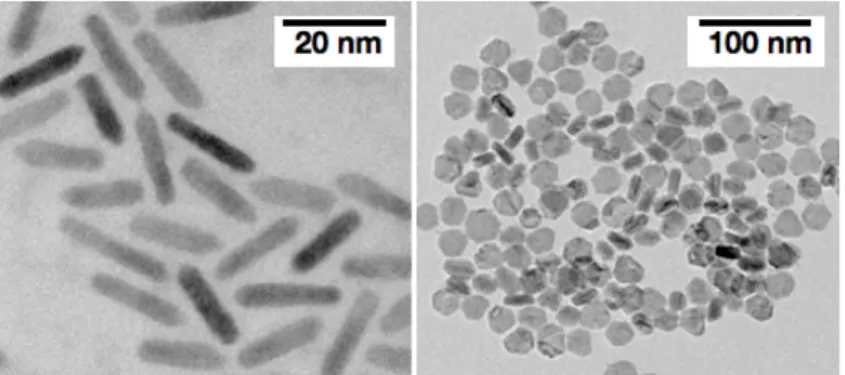
3.1 Example of transmission electron images of rod-like . . . 37
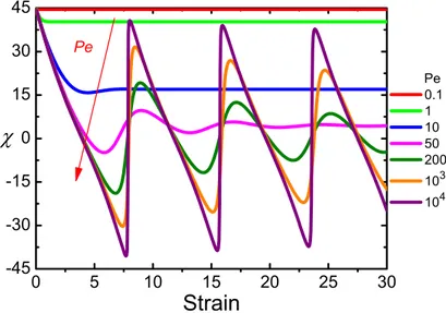
3.2 he orientation angle as a function of strain calculated from the Smolu- chowski equation . . . 40
3.3 Orientation angle as a function of strain . . . 41
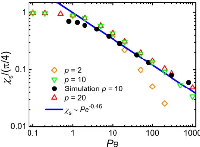
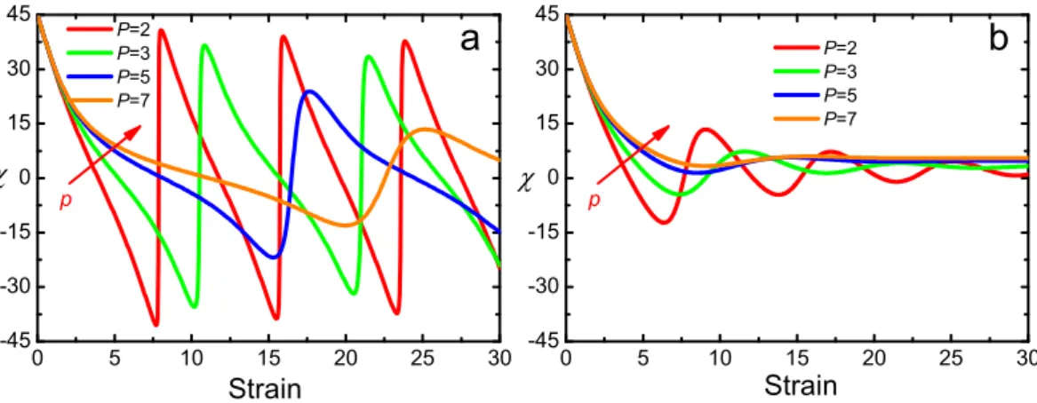
3.4 Normalized asymptotic orientation angle (χs) as a function of P e for p= 2,10 and 20 . . . 42
3.5 Orientation angle as a function of strain at various aspect ratios . . . 43
3.6 Strain at the first half-period as a function of the aspect ratio . . . 43
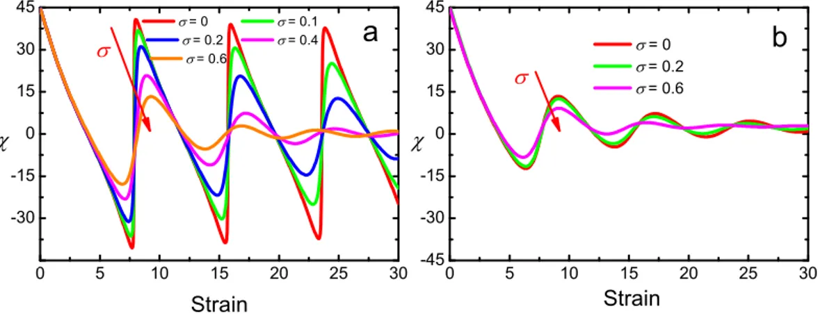
3.7 Orientation angle as a function of strain for varying polydispersity . . . . 44
3.8 Comparison of experimental orientation angle as a function of strain to the prediction . . . 45
3.9 Orientation angle as a function of strain comparing experiments and Smoluchowski equation . . . 46
4.1 The configuration of a spiral object . . . 51
4.2 The geometry of helix varies with parameters . . . 51
4.3 Sketch of a chain segment containing four monomers . . . 52
4.4 Rotational diffusion coefficient of helix . . . 54 xi
4.5 Temporal evolution of the normalized end-to-end length of helix . . . 55
4.6 Diagram of helix state . . . 55
4.7 Average end-to-end length of helix varies with the rigidity of helix . . . . 56
4.8 Changed amplitude of helix length varies with the rigidity . . . 56
4.9 Temporal evolution of the normalizedy label of first bead . . . 57
4.10 Estimated average hydrodynamic aspect ratio, polydispersity, and Peclet number . . . 57
4.11 Tumbling period of helix varies with shear rate . . . 58
4.12 Effective aspect ratio as function ofκ . . . 58
4.13 Temporal evolution of the displacement of helix along vorticity direction . 59 4.14 Temporal evolution of the displacement of helix at different Pelect number 60 4.15 Drift velocity vD as function of Peclet number from 0 to 3×10³. Rota- tional diffusion coefficient of the helixDr= 3.3×10⁻⁵. . . 61
4.16 Drift velocity as a function of the number of helix pitches . . . 61
4.17 Drift velocity as function of radius of helix. . . 62
4.18 Drift velocity varies with the radius of helix under shear rate ˙γ = 0.1. . . 62
4.19 Drift velocity varies with the flexibility of helix . . . 63
5.1 Net rotating motion of a deforming gel helix . . . 66
5.2 Sketch of helix configuration . . . 67
5.3 Illustration of a perfect helix undergoing non-reciprocal deformation with centreline . . . 67
5.4 Schematic of rotational angles . . . 69
5.5 Angular displacement vary with periods. . . 69
5.6 Net rotational displacement generated from a small-radius helix . . . 70
5.7 Angular displacement varies with periods . . . 70
5.8 The time dependence of angular displacement . . . 71
5.9 Average net angular displacement vs. deformation period. . . 72
5.10 Time dependence of the angular displacement . . . 73
5.11 Average net angular displacement (∆θ,∆ϕ) varied with fluid vicosity µ. The net angular displacements are averaged over seven periods in Fig. 5.10 and Fig. 5.5 . . . 74
5.12 Motility map . . . 75
5.13 Time dependence of the angular displacement withNT . . . 75
5.14 Schematic of helix confined by a slit with widthLw/2Lh . . . 76
5.15 Time dependence of the angular displacement . . . 77
5.16 Time dependence of helix mass center inzdirection withNT the number of periods in a slit . . . 78
5.17 Time dependence of helix mass center inzdirection withNT the number of periods in a slit . . . 78
2.1 Parameters in simulation . . . 29 3.1 Physical dimensions of the five analyzed samples of quantum dots . . . 36 3.2 Estimated average hydrodynamic aspect ratio, polydispersity, and Peclet
number . . . 46 4.1 Different geometries of helix . . . 57 5.1 Solvent kinetic viscosity µvaried by MPC parameters collision time step
h and stochastic rotation angleα. . . 73
xiii
Greek Symbols
α Stochastics rotation angle αh Helix angle
χs Orientation angle
˙
γ Shear rate ηs Viscosity
κbond, κbend, κtors Bond, bending, torsional force constants µ Kinetic viscosity
ω Angular velocity
φ Phase between the two oscillations σ Degree of polydispersity
τ Torsional angle θ Bending angle
Matrix or tensors
Γ Gradient velocity tensor
<ˆ Rotational Operator ˆI Identity tensor
Ω Velocity gradient tensor of simple shear flow σs Stress tensor
xv
T Deviatic stress tensor
E Velocity gradient tensor of elongational flow G Velocity gradient tensor
Roman Symbols
2l Total length of helix ULJ Lennard-Jones potential X Location of monomer c Pitch of helix
CT, CN Coefficient of drag forces Dr Rotational diffusion coefficient Dk Parallel diffusion coefficient D⊥ Perpendicular diffusion coefficient f Deformation frequency of helix h Collision time step
Le End-to-end length of helix M Mass of monomer
m Mass of solvent particle p Aspect ratio of rod
P(r, t) Probability density function P er Peclet number
P er Pressure R Radius of helix Re Reynolds number s Arc length of helix T Tumbling period
t time
TH Deformation period of helix Wuˆ(t) Mean-squared displacement Vectors
ˆ
u Long axis of particle ˆ
v Velocity of particle ˆ
vk Parallel component of velocity of particle vˆ⊥ Perpendicular component of velocity of particle D Diffusion tensor
Fs,Fh,FBr Force g Pressure tensor
Mθ Strength of the vector field r Position of particle
U Flow velocity
Introduction
Colloidal suspensions are systems of particles immersed in a solvent, also commonly referred to ascomplex f luids, in which the solute particles move significantly slower than the solvent particles. As shown in Fig 1.1, the sizes of the colloidal particles roughly range from a few nanometers up to the micrometer scale, whereas typical solvent molecules, such as water, are in the ˚Angstr¨om range. In the early day of condensed-matter physics, the observation of the undirected and seemingly erratic motion of colloidal particles has led to a strong backing of the atom hypothesis [1, 2]. As discussed in Ref. [3],
“It has allowed calculation of the size and number of molecules driving the Brownian motion[4]. Despite the undirected and irregular nature of the movements, Einsteins and Smoluchowskis predictions of a linearly growing mean square displacement has been verified by Perrin [1, 2, 4], who was, at the same time, able to calculate Avogadros number”. The huge difference in the typical time scales of motion of a solvent molecule and a colloidal particle leads to a separation of the dynamics. This fact allows one to regard the influence of the suspending medium as a very short-time correlated random process. Moreover, one typically defines the Brownian time, τB, describing the time that is needed for a particle to cover a distance of its own size. Beyond this time, the motion can be considered overdamped, which means that the motion is no longer systematically ballistic in its character.
Figure 1.1: The skematic of colloids’ length scales. The particles from left to right: Au nanoparticles, metal composite particles, Au nanorod+silica shell, core-shell microgels,
porous structure of catalyst . Figure taken from Ref. [5]
1
As a colloidal particle translates or rotates, it induces a fluid flow in the solvent which affects other Brownian particles in their motion. These interactions are mediated via the solvent and standardly called as hydrodynamic interactions, which lead to rich phenomena of particles motion. This dynamics strongly depends on particle shape and relevant examples of our interest are rod-like colloids or structure with chiral symmetry such as helices. Rods tumble and kayak in shear flow [3, 6–9]. Chiral particles migrate in vorticity direction of shear flow [10–12]. Helical microorganisms can translate or rotate in solvent by a non-reciprocal deformation [13–17].
1.1 Application of colloids system
There are plenty of colloidal products in our daily lives as shown in Fig. 1.1, such as dairy products [18], cosmetics and paint, recent advances in chemical synthesis allow production of functional colloids as well as self-propelled or complexly shaped particles [19]. On one hand, there are practical considerations for the use of colloids in a variety of fields, such as microfluidics, material design, pharmaceutics or drug delivery [20]. On the other hand, fascinating systems can be designed to address fundamental relevant questions. Mutually attached spheres, for example, are sometimes referred to as colloidal molecules as they resemble atomic molecules in their shapes and it is possible to control the bond-angles and overall size and shape [21]. Thus, colloids may be regarded as models for atomic or molecular systems, which simplify the investigation of analogous systems due to slower time scales and larger sizes of the particles [22]. Moreover, on this fundamental level, colloids enable the understanding of the mechanisms of phase transitions and arrested states [23].
(a) (b) (c)
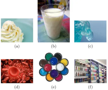
(d) (e) (f)
Figure 1.2: Types of colloids in our daily life. (a) Icecream (b) milk (c) hydrogel (d) blood (e) paints (f) cosmetics. Copy right @ prochemicalanddye.net
1.2 Anisotropic colloids’ shape and non-equilibrium dy- namics
In general, colloidal particles are anisotropic in shape, which was considered in the light of mineral sheets, rod-like viruses and flexible polymer chains by Perrin and Onsager in the 1930s and 1940s [24, 25]. Suspensions of anisotropic particles have been studied by many researchers, e.g. spherocylinders as models for micro-organisms [26, 27]. Recent advances in the chemical synthesis and fabrication of colloidal particles have resulted in a wide variety of shape and size of shape-anisotropic particles, such as rods [28, 29], plates [30], dumbbells [31], hollow objects, microcapsules, patchy particles, cubes [32], octahedra [33], tetrahedra [34], nanostars [35], and colloidal caps, [34] as illustrated in Fig. 1.2.
(a) (b) (c)
(d) (e) (f)
Figure 1.3: Scanning electron micrographs of particles. (a) rod (b) octahedra (c) cube (d) tetrahedra (e) stars (f) cap. Figures taken from [28, 32, 34, 34, 35]
In equilibrium, anisotropy gives rise to novel phases, such as the PC or rotator phase, nematic or liquid crystalline states [36, 37]. At different temperature, for example rod- like liquid crystal molecules exhibits different levels of orientational and positional order as shown in Fig. 1.4. Furthermore, the anisotropy of the suspended particles may be of great importance for dynamical quantities as well as structural formation under external fields [38, 39].
Fascinating phenomena are observed in colloids under the influence of external fields [41]. In processing suspensions, various kinds of external fields are applied to colloids, which may be electrical [42], magnetic [43], also flow fields [44] or gravity [45], to name a few [46]. In fact, even walls or confining boundaries can be seen as a method of external control. The application of external fields can change the equilibrium of the system [47], lead to non-equilibrium steady states or drive the system into full transient non- equilibrium [48]. Under gravity, for example, the coexistence of different phases may be observed due to density gradients [49].
Figure 1.4: Illustration of rod-like liquid crystal molecules exhibiting different levels of orientational and positional order in the crystal, smectic, nematic, and isotropic phases as a function of increasing temperature with melting and clearing points noted.
Figure recreated from [40]]
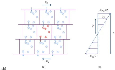
A very important class of external fields are flow fields, which can be quite complex. This spatial or temporal complexity is strongly dependent on the boundary conditions and the driving forces causing media to flow. One of the most elementary flows is the simple shear flow, where the velocity is unidirectional and depends linearly on the distance from the walls. Couette f low is the laminar solution for fluid confined between two plates one of which is moving and the other is fixed at a certain distance with no-slip boundary conditions [50]. Shear flows are very common in processing and transport of material as they are inevitably present due to typical boundary conditions on the flowing medium. In order to analyse the response of a medium to shear, one typically chooses simple shear with an oscillatory or steady time dependence. In the context of colloidal flow, shear can lead to a multitude of phenomena: shear fields may be used to induce crystallisation in colloidal hard sphere glasses, [51] or drive gelation in dilute suspensions of charge-stabilised particles [52]. It may be desirable to prevent crystallisation or glass formation in a process, as solidification can hamper the transport of material. The behaviour of particles under shear have rich phenomena. In Fig. 1.5, for example, semi-flexible polymers exhibit tumbling motion, i.e., they undergo a cyclic stretch and collapse dynamics, with a characteristic frequency which depends on the shear rate and their internal relaxation time [44].
Figure 1.5: Snapshot of semiflexible polymers under shear flow. Figure taken from Ref. [44]
1.3 Rheo-optical approach for particle charaterization
The knowledge of the precise size and shape of colloidal particles is frequently important, as they have a strong effect on the rheological, optical, and/or mechanical properties of suspensions. Preparation of samples for electron microscopy is often laborious and expensive and the analysis of the images is not trivial. Light-scattering methods, as used in many commercial particle-sizing instruments, are not designed to assess particle shapes. Special methods requiring multiple detectors are needed for this purpose, as the angular dependence of the scattered light needs to be analyzed [53]. Measurements of changes in the polarization state of the scattered light provide a possible alternative for nonspherical particles with a given orientation. The establishment of new approaches to determine size and shape of colloids is therefore timely and relevant.
Particle dynamics is governed by the particle geometry, which for example determines the manner of rotation in the flow. For a given particle, the angular velocity is not necessarily constant in time. If the particle is elongated it slows down as its orientation approaches the flow direction and it increases whne it is not oriented. It has been shown that polarimetry measurements of birefringence and especially linear conservative dichroism can be used to study the dynamics of dilute colloidal suspensions in simple shear flow [54–56] .
Linear conservative or scattering dichroism is a property related to anisotropic scattering of light. It is defined as the difference in the principal eigenvalues of the imaginary part of the refractive-index tensor. In a dilute system of nonspherical particles, the magnitude of the linear conservative dichroism reflects the degree of alignment induced by the shear flow. Here, however, it is more convenient and simple to consider evolution of the average orientation angle χ, which is given by the projection of the principle axis of the imaginary part of the refractive-index tensor in the flow-velocity gradient plane.
It is a purely geometrical property, the determination of which is not affected by the size for samples with uniform optical properties. For that reason it is more suited to characterize suspensions of nonspherical particles. Existing methods have shown that the combination of rheo-optical approach and theoretical results of particle orientation can obtain aspect ratios and polydispersity of particles under assumptions of nearly spherical particles, narrow distribution of size, negligible Brownian motion [57, 58] illustrated in Fig. 1.3.
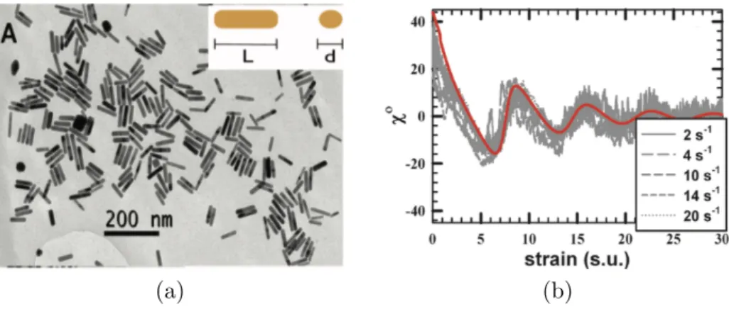
(a) (b)
Figure 1.6: (a) Transmission electron micrographs of nonspherical gold nanoparticles.
(b) Orientation angleχ as a function of strain for (a). Figures taken from Ref. [58]
1.4 Motion of chiral objects
A chiral object has two distinct forms that are mirror images to each other, but each can not be converted into the other by pure spatial rotations as shown in Fig. 1.7. The study of the dynamics and interactions of chiral obejcts is an interesting and fascinating subject. The pioneering observation by Louis Pasteur in 1848 linked the chirality of the sodium ammonium salt crystals to light polarization [59]. Chirality in macromolecules has led to many important structural properties, especially in liquid crystals [60]. As for example, the double helix of DNA is chiral and always right handed [61]. All but one of natural amino acids, the building blocks of proteins, are chiral and are only in the left-handed forms. Many other molecules important to life are chiral, and it is still a mystery why only one of the two enantiomers is used by living organisms [62].
Figure 1.7: Illustration of chirality by helices. Figure taken from Ref. [63]
Recently, synthetic helical particles at the nanoscale, with radii smaller than 100nm have become available [64, 65]. Controlled and directed motion of chiral particles has important applications as in the case of targeted delivery of genetic material and drugs, this is since such particles can be tailored to facilitate their efficient uptake by various cells or tissues. Controlled motion and cargo transport of magnetic helical particles has been demonstrated [43]. Application of time-dependent magnetic fields on magnetic screw-like particles induces a torque that rotates the particle and propels it in the fluid.
Manipulation of the direction of the rotating magnetic fields makes it possible to load microspheres as cargo into the holder of a helical particle, transport the cargo and then release it at a preferred site [43]. In the interesting work shown in Fig. 1.8, externally
driven microhelices can be used to assists sperm to delivery on immotile live cell [66], see Fig. 1. 8.
Figure 1.8: (i) Sperm cell captured by by magnetic helcal micro particle (ii) transport (iii) approach to the oocyte membrane (iv) and release. Figure taken from Ref. [66]
Chemical syntheses of chiral molecules in laboratories usually produce roughly equal amounts of the two enantiomers, such that separation of enantiomers becomes an im- portant issue inspite of difficult process. Currently, the main methods consist in driving the enantiomer mixtures through specific chiral filling materials, often with not so satis- factory efficiencies [67, 68]. Motion and kinetics of chiral objects are largely determined by their spatial anisotropy since it leads to a coupling between the translational and rotational degrees of freedom. De Gennes already suggested dragging by external forces an enantiomer crystal along the surface of a liquid or solid [69]. As illustrated in Fig.
1.9, the friction on helix under shear could then produce a chiral-specific lateral forces, although it was noted that the crystal needs to be macro-sized to overcome the thermal fluctuations. It was then proposed that a microfluidic flow with spatially varied vortic- ity could separate enantiomers, due to intricate interplay between the particle transport and thermal fluctuating diffusive motions [70].
Figure 1.9: Motion of chiral particles placed in shear flow. If the particle P moves with the velocityVin the shear flow, the mirror-imaged particle P will move with the
velocityV0, which is the mirror image of V. Figure taken from Ref. [71]
1.5 Microswimmer at low Reynolds number
Active matter is a fascinating new field in soft matter physics. It concerns the macro- scopic properties of interacting active particles, which are individually able to convert energy into directed motion. As disccussed in Ref. [72], “Locomotion is a major achieve- ment of biological evolution and is an essential aspect of life. Search for food, orientation toward light, and spreading of the own species are only possible due to locomotion. The spectrum of biological active system in microscopic world is vast, ranging from sperma- tozoa [73], bacteria [72, 74], to the cytoskeleton in living cells [75–78]. Yet, highly active systems are not just limited to examples from nature and the development of synthetic microswimmers is recently making an enormous progress [79]”. Hence, studying the dynamics of active matter is a key element on the way to a better understanding of autonomous biological systems, the development of novel biomedical technologies, and new designs of microfluidic devices. A common characteristics of active matter is the utilization of energy from the environment for, or the internal conversion of chemical energy into, directed propulsion [72, 74, 79–83].
The physics of microswimmers is fairly different from that we experience in our macro- scopic world. While for, e.g., swimming humans, inertia is dominating over the viscous forces, for microswimmers it is the other way around. The ratio between the inertial and viscous forces is known as Reynolds number. The value of the Reynolds number spans over several orders of magnitude from 106 of swimming humans to 10−5 of bacteria. At high Reynolds numbers, the momentum transferred from the swimming body to the sur- rounding fluid convects and slowly dissipates from larger to smaller length scales. At low Reynolds numbers there is almost no inertial delay in time between the applied forces and the fluid response. Therefore, at zero Reynolds number, every reciprocal motion, i.e., every periodic motion, which after time reversal is identical to its original dynamics, will not lead to self-propulsion. This property is known as the scallop theorem [14, 82].
Artifical microswimmers can be constructed by using similar design principles as those found in biological systems. As explained in Ref. [72], “A by now classical example is a swimmer which mimics the propulsion mechanism of a sperm cell [84]. The flagel- lum is constructed from a chain of magnetic colloid particles and is attached to a red blood cell, which mimics the sperm head. This artificial swimmer is set into motion by an alterating magnetic field, which generates a sidewise oscillatory deflection of the flagellum. However, the swimming motion is not the same as for a real sperm cell; the wiggling motion is more a wagging than a travelling sine wave, and generates a swim- ming motion toward the tail end, opposite to the swimming direction of sperm. A recent example of a biohybrid swimmer which mimics the motion of sperm has been presented by Williamset al. [85]. In this case, the microswimmer consists of a polydimethylsilox- ane filament with a short, rigid head and a long, slender tail on which cardiomyocytes (heart-muscle cells) are selectively cultured. The cardiomyocytes contract periodically and deform the filament to propel the swimmer. This is a true microswimmer because it requires no external force fields. The swimmer is about 50 µm long and reaches a swimming velocity up to 10 µm/s”. A more recent experimental work [86] has shown for the purposefully shaped microhydrogels that the kinematics of a cyclic body shape
variation can be tuned to differentiate between the forward and the backward motion as shown in Fig. 1.5. Thus, the first deformation stroke (upon heating) is not reciprocated by the second deformation stroke (during cooling), even though the cycle ends up at its starting configuration. Based on this, a light-fueled and light-controlled microswimmer has been designed, which can rotate and move forward by its body deformation.
(a) (b)
Figure 1.10: Actuation characteristics of a microgel ribbon helix under stroboscopic irradiation. a) Microscopy images from time-lapse videos of the helix during irradiation.
b) Instantaneous helix length and diameter during one irradiation cycle. The left part corresponds to when the light is on, while the right part corresponds to when the light
is off. Figures taken from [86]
1.6 Objectives and outline of the thesis
Chapter 2: The related theoretical framework will be introduced by including the dynamics of shape-anisotropic colloids, hydrodynamics in Stokes regime, and some the- oretical methods applied in microswimmers. Then a hybrid simulation method will be introduced, which combines multi-particle dynamics with molecular dynamics.
Chapter 3: Since the hydrodynamic aspect ratios and polydispersity of particles are im- portant for the application of nano-particles, a charaterization technology is developed.
The Smoluchowski equation can be generalized on arbitrary aspect ratios, polydispersity, and include thermal fluctuation, which goes beyond the limits of the existing methods [57, 58]. The numerical results of Smoluchowski equation contain the shear rate, the equivalent hydrodynamic aspect ratio, and the associated polydispersity. Then they can be obtained from a fit to the experimental data, as will be demonstrated for a model system containing quantum dots.
Chapter 4: The non-equilibrium dynamics of helix have been studied [11, 45, 71]. For example, the study has shown that twisted ribbons can be separated by shear flow as illustrated in Fig. 1.6. Previous studies are still restricted to rigid particles or flexi- ble tetrahedron. Therefore, open questions still include how the chiral geometry and flexibility of helix affect the efficiency and migration speed. We address these issues by Molecular dynamics coupled Multi-particles dynamics simulation [87, 88], which intrin- sically involve thermal fluctuations hydrodynamic interactions and varying flexibility.
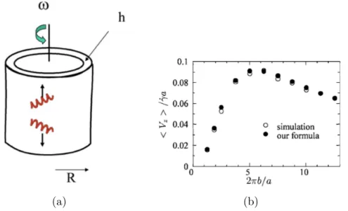
(a) (b)
Figure 1.11: (a) Sketch of the rheological separator. (b) Mean migration velocity of twisted ribbon of length in the limit of large Peclet number is plotted against the pitch.
Figures taken from Ref. [71]
Chapter 5: Aritifical microswimmers have a huge potential applications in drug delivery and micro-robots. Recent experimental work developed a novel gel which can deform by responsing to temperature as shown in Fig. 1.5. As a results the actively driven helix has a net rotation. Later theoretical work [89] demonstrated that the net rotation is due to non-reciprocal deformation of helix. However, the effect of fluid viscosity and walls on the swimming and migration of helix was not considered. Therefore, we investigate these issues, including the effect of helix configuration, fluid viscosity, deformation periods on the propulsion of helix herein by the same former simulation method.
Theoretical background and simulation Methods
2.1 Theoretical Background
2.1.1 Dynamics of dilute non-spherical colloids
Shear flow is typical case where the dynamical behavior can be investigated in a station- ary nonequilibrium state. Shear flow affects microstructural order of colloidal systems in two respects : center-to-center correlations are affected by flow and flow can induce changes in orientational order. For spherical colloids, flow-induced changes of macro- scopic properties find their origin entirely in shear-induced changes of center-to-center correlations. For non-spherical colloidal particles, flow also tends to align single col- loidal particles due to the torque that the flowing solvent exerts on their cores. For very elongated colloids, single particle alignment is dominant over shear-induced changes of center-to-center correlations. For such systems, equations for one-particle orientational distribution functions, with the neglect of flow-induced distortions of center-to-center correlations, are sufficient to predict their macroscopic behaviour under flow. For spher- ical colloidal particles, however, one-particle distribution functions are not affected by flow, so that theory for spheres should be based on equations for correlation functions.
2.1.1.1 The velocity gradient tensor
A linear flow profile is characterized by means of the velocity gradient tensorG, where the flow velocity U at position r is written as U =G·r. In case of simple shear flow, the gradient velocity tensor is usually denoted as Γ, and is equal to
Γ= ˙γ
0 1 0 0 0 0 0 0 0
, simple shear flow. (2.1)
11
Figure 2.1: (a) Simple shear flow. (b) Elongational flow, sometimes also referred to as extensional flow (where the elongational and compression axes are indicated), and
(c) Rotational flow. Arrows indicate the flow direction.
The corresponding flow profile is a flow in the x-direction, with its gradient in the y- direction, as sketched in Fig. 2.1a. The z-direction is commonly referred to as the vorticity direction. The strength of the flow is characterized by the shear rate , which equals the spatial gradient∂Ux/∂y of the flow velocity Ux in the x-direction. For elon- gational or extensional flow, the velocity gradient tensor is denoted as E, and reads,
E = 1 2γ˙
0 1 0 1 0 0 0 0 0
, elongational flow. (2.2)
the corresponding flow is sketched in Fig. 2.1b. In such an elongational flow, deformable objects tend to elongate along the so-called extensional axis, and compressed along the compressional axis. With this coordinate these two directions are in the diagonal ofx−y axis as indicated in fig. 2.1b. Whenever it is not specified whether simple shear flow or elongational flow is considered, the velocity gradient tensor can be generally denoted as G.
It is instructive to use velocity calculus method, which allow to decouple any arbitrary matrix in its symmetry GS and asymmetry GA parts G, G = GS+GA with GS =
1
2(G+GT) and GA= 12(G−GT), where the superscript T stands for the transpose of the corresponding tensor. For elongational flow, the velocity gradient tensor is already symmetric, such that GS = E and GA =0 . For simple shear flow we have GS = 12E and GA= 12ΩwithΩthe rotation matrix:
Ω= 1 2γ˙
0 1 0
−1 0 0
0 0 0
, simple shear flow (2.3)
The flow velocities corresponding to rotational flow in Eq. 2.3 are sketched in fig. 2.1c, Note that,
Γ=E+Ω (2.4) so that simple shear flow can be decomposed into a linear combination of elongational and rotational flow, which is relevant to explain the rotate polymer dynamics.
2.1.1.2 Translational diffusion
For non-spherical colloids, the friction coefficient is not isotropic since it depends on the orientation of the rod/plate relative to it’s velocity. The orientation of a rod is characterized by a unit vector ˆu along it’s long axis (see Fig. 2.2a). When the rod moves through the fluid along ˆu, the friction coefficientζ|| is different from the friction coefficientζ⊥ when the rods moves in a direction perpendicular to ˆu. A velocity vwith arbitrary direction can be decomposed in it’s components vk parallel to it’s long axis and it’s perpendicular componentv⊥. The parallel component is equal to vk = ˆuuˆ·v, while the perpendicular component is equal to v⊥ = v−vk = [ˆI−uˆu]ˆ ·v (where ˆI is the identity tensor). The friction force Fh is thus equal to [90],
Fh =−ζkvk−ζ⊥v⊥ =−n
ζkuˆˆu+ζ⊥
hˆI−uˆˆu io
· v, (2.5)
A colloid moving in a fluid with constant velocity has no net applied force such that Fh+FBr= 0 (where the superscript ”Br” stands for ”Brownian”),
FBr=−kBT∇lnP(r, t). (2.6)
By combination of Eq. 2.5 and Eq. 2.6, we can get
v=−D(ˆu)· ∇lnP(r, t), (2.7)
with the diffusion tensor
D=Dkuˆˆu+D⊥
hˆI−uˆuˆi
(2.8) where P(r, t) is the probability density function (pdf) of colloid the center-of-mass po- sition r= (x, y, z) of a colloidal particle, at time t and,
Dk= kBT ζk
, D⊥= kBT ζ⊥
. (2.9)
are the parallel and perpendicular diffusion coefficients. According the continuty equa- tion [91, 92], we thus finally arrive at the diffusion equation for translational motion of a non-sperical particle,
∂
∂tP(r, t) =∇ ·D(ˆu)· ∇P(r, t) (2.10) The most simple average that characterizes Brownian motion is the so-called mean− squared displacement W(t) =
r2
(withr=|r|the distance of the center-of mass from the origin). W(t) can be calculated by first multiplying Eq. 2.10 on both sides withr2. Since W(t= 0) = 0, this implies that,
W(t) = 6Dt. (2.11)
In order to analyze the motion of a rod we therefore need a similar diffusion equation for the orientation of the rod.
2.1.1.3 Rotational diffusion
For non-spherical macromolecules it is not only the center-of-mass that exhibits random Brownian motion due to collisions with fluid molecules, but also it’s orientation changes as a result of these interactions.
We consider a rod-like Brownian particle, the orientation of which is specified by a unit- vector ˆu. For a rod-like particle this vector lies along the long axis of the rod, while for a platelet this vector can be chosen to be perpendicular to the face of the platelet (see Fig.
2.2)a The tip of the unit-vector ˆulies on a unit-spherical surface. Changes in orientation leads to motion of the tip of ˆu. on a unit-spherical surface (as depicted in Fig. 2.2b). We define the probability density function (pdf) P(ˆu, t)dˆu is the probability that ˆu takes a value within the small surface area element dˆu on the unit-spherical surface (see Fig.
2.2c). The rotational diffusion equation:
∂
∂tP(ˆu, t) =DrRˆ2P(ˆu, t) (2.12) whereDr is rotational diffusion coefficient. The rotational operator is defined as,
R(· · ·) = ˆˆ u× ∇uˆ(· · ·) (2.13) The time dependence of the average of the orientation vector ˆu can be obtained from Eq.2.12 by multiplying both sides with ˆuand integrating over the unit-spherical surface,
dhˆui(t) dt =Dr
I
dˆuˆuRˆ2P(ˆu, t) =Dr I
dˆuP(ˆu, t) ˆR2uˆ =−2Drhuiˆ (t) (2.14) A partial integration is performed in the second equality. The orientational equivalent of mean-squared displacement is Wˆu(t) =
D
|ˆu−uˆ0|2E
, where ˆu0 is the orientation of the particle at the initial time. From the above results is found that,
hbt!
Figure 2.2: (a) A platelet (left) and rod-like (right0 colloidal particle, where the unit vector ”ˆu” defines their orientations. (b) The tip of the unit vector ˆu, in red, lies on an unit-spherical surface (the surface of as sphere with radius unity). The red ”point- particle” exerts Brownian motion on the unit-spherical surface. (c) The orientations of
two rods are mimicked as different points on the unit-spherical surface
Wuˆ(t) = ˆ u2
+ ˆu20−2huiˆ uˆ0= 2 [1−exp{−2Drt}] (2.15) For small times, with Drt 1, Wuˆ(t)is the displacement of the tip of ˆu on the two- dimensional plane perpendicular to ˆu0. Expanding the exponent function (using that expx = 1 +x+· · · ) leads to Wu(t)ˆ = 4Drt, which indeed complies to Eq. 2.11 for translational diffusion in two dimensions.
2.1.1.4 Diffusion in the presence of shear flow
In the present section we discuss probability density functions (pdfs) and orientational order parameter matrices for a single Brownian rod subjected to flow. On applying a stationary flow, the orientational pdf of a single rod attains a stationary form. This time independent pdf is determined by the interplay of the aligning effect of the flow and isotropy-restoring rotational diffusion. The stationary form of the Smoluchowski equation [91] for a single rod reads,
0 = ˆR2P(ˆu)−P erR ·ˆ [P(ˆu)ˆu×(G·u)]ˆ , (2.16) where the dimensionless parameterP eris commonly referred to as the rotational Peclet number, which is defined as,
P er= ˆγ Dr
(2.17) This Peclet number is a measure for the effect of the shear flow relative to isotropy- restoring rotational diffusion. For small Peclet numbers, rotational diffusion is relatively fast, so that the pdf is only slightly anisotropic.
The stationary equation of motion can be solved in closed analytical form when the velocity gradient tensor G is symmetric (as for elongational flow). When the velocity gradient tensor is not symmetric (as for simple shear flow), the solution cannot be obtained in a simple closed analytical form, but must be obtained by numerical methods.
However, expansion of the orientational pdf for small Peclet numbers is feasible.
In case of shear flow and for small rotational Peclet numbers the deviation of the pdf from the isotropic solution is small, so that the solution of the stationary equation of motion 2.16 can be expanded as,
P(ˆu) = 1
4π +P erP1(ˆu) +P e2rP2(ˆu) +· · ·. (2.18) Substitution of this expansion into Eq. 2.16 and equating coefficients of equal powers of P er, one readily finds the following recursive set of differential equations for the as yet unknown functions Pj,
Rˆ2Pj(ˆu) = ˆR ·[Pj−1(u)u×(Γ·u)] , j≥1, (2.19) where P0(ˆu) = 1/4π is the isotropic pdf without shear flow. Normalization requires that,
I
dˆuPj(ˆu) = 0 , j ≥1. (2.20) Let us consider the first two terms in the expansion 2.18. Forj= 1, using that P0(ˆu) = 1/4π, Eq. 2.19 reads,
Rˆ2P1(ˆu) = 1 4π
R ·ˆ [ˆu×(Γ·u)] =ˆ − 3
4π (ˆu·E·u)ˆ , (2.21) where ˆE is the symmetric part of the gradient velocity tensor ˆΓ in Eq. 2.1, that is, Eˆ = 12(ˆΓ + ˆΓT). The above equation follows from the relations given in [91, 92]. Using these relations once more immediately leads to the expression in a spherical coordinates,
P1(ˆu) = 1
8π (ˆu·E·u) =ˆ 1
8π sin2(θ)sin(φ)cos(φ), (2.22) Substitution of this solution forP1 into Eq. 2.19 for j= 2 yields,
Rˆ2P2(ˆu) = 1 8πR ·ˆ h
(ˆu·E·u)ˆ
uˆ×Γˆ·uˆ i
= 1 8π
uˆ2−5(ˆu·E·u)ˆ 2
. (2.23) The solution to Eq. 2.23 is given by,
P2(ˆu) = 1 32π
(ˆu·E·uˆ+1
3(ˆu21−uˆ22)− 1 15)
= 1 32π
sin4(θ) sin2(φ) sin2(φ) +1
3sin2(θ)(cos2(φ)−sin2(φ))− 1 15
,
(2.24)
The constant 1/15 between the square brackets is the result of considering the normal- ization constraint 2.20.
Summarizing the previous results, we thus obtain the following small Peclet number expansion (valid up to O(P e3r)),
P(ˆu) = 1
4π +P er 1
8π (ˆu·E·u) +ˆ P e2r 1 32π
(ˆu·E·uˆ+1
3(ˆu21−uˆ22)− 1 15)
(2.25)
For small Peclet numbers, rods spend most of their time in a direction where χ = 45◦ (angle between the director and the flow direction) and eventually perform some rotations. This is the result of the interplay between the Brownian torque on the rod and the torque that the fluid exerts on the rod. A preferred alignment along the flow direction implies a strongly peaked orientational pdf. Brownian torque tends to diminish the strongly peaked pdf in the flow direction, while the fluid torque tends to make it more peaked [90, 91].
2.1.2 Hydrodynamics
Most every day soft matter systems, such as gel-like structures, are typically multi- component systems, and the forming objects, polymers, colloids, etc. are dissolved in a fluid solvent. This fluid significantly influences or even dominates the dynamical behavior of the embedded objects. Fluid motion induced by the displacement of the embedded particle leads to a dynamical response of other particles due to the long- range character of the fluid-mediate interactions. Those are the well-know hydrodynamic interactions.
A theoretical description of hydrodynamic interactions is challenging because of the large length-scale difference between a fluid particle, e.g., a water molecule, and the embedded nano- to micro-meter size particle. Hence, the fluid is often described in terms of linearized Navier-Stokes equations, which can be solved analytically.
2.1.2.1 Navier-stokes equations
The Navier-Stokes equations on large length and time scales of an incompressible fluid determind the mass and momentum conservation of a fluid element and read as [91, 93]:
ρ∇u= 0, (2.26)
ρ ∂u
∂t + (u· ∇)u
=−∇ps+ηs∇2u+f(t) (2.27) where ps and ηs are pressure and solvent viscosity, respectively. The terms ρ and u = u(r, t) are mass density and velocity field of the fluid at position r and time t, respectively. Eq. 2.26 is the mass conservative or continuity equation. Eq. 2.27 is the conservative of momentum equation. The additionally assumed incompressibility, which is justified in most applications. The nonlinear term (u· ∇)u is the convection acceleration of fluid. The left hand-side of equation 2.27 expresses the inertia for the system. The term−∇pis the pressure gradient. The sign indicates that the force on the fluid is towards the lower pressure. The termηs∇2uis the viscous friction forces which appear as restricting forces due to velocity gradients within the fluid. Viscous friction and pressure gradient (−∇ps+ηs∇2u) follow by the divergence from the stress tensor, which is defined as
σs=psI+T (2.28)
The tensors I and T are the identity tensor and deviatoric stress tensor, respectively.
The gradient of the shear stress tensor gives ηs∇2u. The last term in equation 2.27, f(t), is related with any external volume force, e.g., gravity.
2.1.2.2 Stokes equation
In order to analyze the contributions of the various terms in the Navier-Stokes equations, we rescale
u0 =u/V0,r0 =r/L0, t0=t/T0 (2.29) whereV0 is a typical velocity,L0is a typical length andT0is the timescale of the problem at hand. In those new variables and after multiplying by L20/(ηsV0), the Navier-Stokes equations read
ρL20 ηsT0
∂u0
∂t0 + Re u0·(∇0u0) =−∇0p0s+ ∆0u0+ f0(t) (2.30) where we defined the dimensionless pressure p0 =L20η−1V0−1p, the dimensionless force f=L20η−1s V0−1f, and ∇0 =∂/∂r0. Furthermore, we introduced a dimensionless number, the Reynolds number Re
Re = ρV0L0
ηs , (2.31)
For Re 1 we can neglect the nonlinear advective term in Eq. 2.27, yielding the linearized Navier-Stokes equations
ρ∂u
∂t =−∇p+η∆u+f (2.32)
For small Reynolds numbers and on the diffusive time scale, the Navier-Stokes equation 2.26 and 2.27, therefore simplifies to,
0 =∇ ·u (2.33)
0 =−∇p+η∆u+f (2.34)
The Stokes equations are also known as creeping flow equations. They are time-independent and linear. The latter allows for superposition of solutions, which greatly simplifies the theory. To describe hydrodynamic interactions, where nano- to micrometer size objects are dissolved in a fluid, the convection term is typically neglected, i.e., low Reynolds number fluids are considered [91], or the inertia term is neglected and Eq. 2.27 turns into the Stokes equation.
2.1.2.3 The Oseen tensor
An external force acting on a single pointr0 of the fluid is mathematically described by a delta distribution,
fext(r) =f0δ(r−r0) (2.35)
The prefactor f0 is total force R
dr0fext(r0) acting on the fluid. Since the creeping flow equations are linear, the fluid velocity at some pointrin the fluid, due to the point force inr0, is directly proportional to that point force. Hence,
u(r) =To(r−r0)·f0 (2.36) The tensorTois commonly referred to as the Oseen tensor,. The Oseen tensor connects the point force at a point r0 to the resulting fluid flow velocity at a point r. Similarly, the pressure at a pointr is linearly related to the point forces,
p(r) =g(r−r0)·f0 (2.37)
The vector g is referred to here as the pressure vector.
Consider an external force which is continuously distributed over the entire fluid. Due to the linearity of the creeping flow equations, the fluid flow velocity at some point ris simply the superposition of the fluid flow velocities resulting from the forces acting in each point on the fluid. Hence,
u(r) = Z
d(r0T(r−r0)·fext(r0) (2.38) The same holds for the pressure,
p(r) = Z
d(r0g(r−r0)·fext(r0) (2.39) substitute Eqs. 2.38 and 2.39 into the creeping flow equations (2.34, 2.33), leads to,
∇ ·T(r) =0 (2.40)
∇2g(r)−η0∇2T(r) =Iδ(r) (2.41)
2.1.3 Models for filamentous swimmer
Exact analytic results for the drag coefficients of certain high-symmetry shapes such as spheres and ellipsoids can be obtained in the Stokes limit. For more complex shapes such as chiral particles, the boundary integral formulation of the Stokes equation can be used [94–96], which reduces the full three-dimensional problem of solving for the fluid flow to the two-dimensional problem of determining source distributions on the bounding surfaces. The typical Reynolds number in experiments of driven magnetic helices at the micron scale and at the nanoscale are about 10−8 and 10−9 [97]. Hence zero Reynolds number approximation is justified. The resistive force theory (RFT) and the slender body theory (SBT) are the usual approaches used to study the propulsive motion of rigid helices and flagellar propulsion.
2.1.3.1 Resistive force theories
In the 1950s, Gary and Hancock [98] developed resistive force theory to provide a de- scription of HI applied to flexible filaments. It represented a breakthrough in the theory of Stokes flows, which is still widely used [99–101].
In formulating resistive force theory, the filament is assumed to be thin, with a circular cross section. In this way, one can first consider an average force per unit length acting on the filament centerlines, rather than a force per unit area acting over the surface.
In addition, the cross-sectional symmetry allows us to consider just two independent,
Figure 2.3: A two-dimensional representation of the resistive force theory approxima- tion. The local velocity of a slender filament of circular cross section can be separated into components tangential and perpendicular to the filament. Figure cited from [102]
non-trivial coefficients CN and CT relating forces to velocities for the filament in the normal and tangential directions, since the binormal and normal are interchangeable.
Decomposing the local filament velocity into its normal, tangential, and binormal direc- tions, i.e., v= vN+vT+vB, with an analogous expression for the local viscous force per unit length acting on the filament, f = fN+fT+fB, then resistive force theory formally states that the local viscous drag forces and filament velocities are related by
fT=−CTvT, fN=−CNvN, fB=−CNvB, (2.42) Simple kinematical and symmetry arguments based on linearity are sufficient to demon- strate that a linear, symmetric tensor relates viscous drag to velocity for a sufficient long, straight cylinder, and thus, via a suitable choice of axes, such that the above equation emerges. However, the power of resistive force theory is the demonstration that these relationships hold locally for any slender body with circular cross section, at least to logarithmic accuracy in the body aspect ratio, given appropriate estimates for CN and CT.
For a filament of length L, the net viscous force and net torque are given by
F(t) = Z L
0
f(s)ds=−CN Z L
0
vN(s)ds−CN Z L
0
vB(s)ds−CT Z L
0
vT(s)ds (2.43)
and
M(t) = Z L
0
X(s)×f(s)ds=−CN Z L
0
x(s)×vN(s)−CN Z L
0
X(s)×vB(s)ds
−CT Z L
0
X(s)×vT(s)ds
(2.44)