Maxima by Example: Ch. 2, Plots, Files, Read, Write, and Fit ∗

(1)

Ch. 2, Plots, Files, Read, Write, and Fit

^∗

Edwin L. Woollett January 6, 2014

You should be able to use any of our examples with either wxMaxima or Xmaxima. If you substitute the wordwxplot2dfor the wordplot2d, you should get the same plot (using wxMaxima), but the plot will be drawn “inline” in your notebook rather than in a separate gnuplot window, and the vertical axis labeling will be rotated by 90 degrees as compared to the gnuplot window graphic produced byplot2d.

To save a plot as an image file, using wxMaxima, right click on the inline plot, choose a name and a destination folder, and click ok.

The XMaxima interface default plot mode is set to “Separate”, which the author recommends you use normally. You can check this setting in the XMaxima window by selecting Options, Plot Windows, and see that Separate is checked. (You can then back out by pressing Esc repeatedly.)

To save a XMaxima plot drawn in a separate gnuplot window, left click the left-most icon in the icon bar of the gnuplot window, which is labeled “Copy the plot to clipboard”, and then open any utility which can open a picture file and select Edit, Paste, and then File, Save As. A standard utility which comes with Windows XP is the accessory Paint, which will work fine in this role to save the clipboard image file. The freely available Infanview is a combination picture viewer and editor which can also be used for this purpose. Saving the image via the gnuplot window route results in a larger image.

We discuss later how to use an optional plot2d list to force a particular type of image output. A simple example is plot2d (sin(u),[’u,0,%pi], [gnuplot_term,’pdf])$

which will create the image filemaxplot.pdfin your current working directory.

2.1.1 First Steps with plot2d The syntax ofplot2dis

plot2d( object-list, draw-parameter-list, other-option-lists).

The required object list (the first item)maybe simply one object (not a list). The object types may be expressions (or functions), all depending on the same draw parameter, discrete data objects, and parametric objects. If at least one of the plot objects involves a draw parameter, sayp, then a draw parameter range list of the form[p, pmin, pmax]should follow the object list.

We start with the simplest version which only controls how much of the expression to plot, and does not try to control the canvas width or height.

(%i1) plot2d ( sin(u), [’u, 0, %pi/2] )$

which produces (on the author’s Windows XP system) approximately:

0 0.2 0.4 0.6 0.8 1

0 0.2 0.4 0.6 0.8 1 1.2 1.4

sin(u)

u

Figure 1: plot2d ( sin(u), [’u, 0, %pi/2] )

(4)

While viewing the resulting plot, use of the two-key commandAlt-Spacebar, which normally (in Windows) brings up a resizing menu, instead switches from the gnuplot figure to a raw gnuplot window. You can get back to the figure using Alt-Tab, but the raw gnuplot window remains in the background. You should resize the figure window by clicking on the Maximize (or Restore) icon in the upper right-hand corner. Both the figure and the raw gnuplot window disappear when you close (using, sayAlt-F4, twice: once to close the figure window, and once to close the raw gnuplot window).

Returning to the drawn plot, we see that plot2d has made the canvas width only as wide as the drawing width, and has made the canvas height only as high as the drawing height. Now let’s add a horizontal range (canvas width) control list in the form[’x,-0.2,1.8]. Notice the special role the symbolxplays here inplot2d.uis a plot parameter, andxis a horizontal range control parameter.

(%i2) plot2d ( sin(u),[’u,0,%pi/2],[’x, -0.2, 1.8] )$

which produces approximately:

0 0.2 0.4 0.6 0.8 1

0 0.5 1 1.5

sin(u)

u

Figure 2: plot2d ( sin(u), [’u, 0, %pi/2], [’x,-0.2,1.8] )

We see that we now have separate draw width and canvas width controls included. If we try to put the canvas width control list before the draw width control list, we get an error message:

(%i3) plot2d(sin(u),[’x,-0.2,1.8], [’u,0,%pi/2] )$

set_plot_option: unknown plot option: u

-- an error. To debug this try: debugmode(true);

However, if the expression variablehappensto bex, the following command includes both draw width and canvas width using separatexsymbol control lists, and results in the correct plot:

(%i4) plot2d ( sin(x), [’x,0,%pi/2], [’x,-0.2,1.8] )$

in which the first (required)xdrawing parameter list determines the drawing range, and the second (optional)xcontrol list determines the canvas width.

Despite the special role the symbolyalso plays in plot2d, the following command produces the same plot as above.

(%i5) plot2d ( sin(y), [’y,0,%pi/2], [’x,-0.2,1.8] )$

(5)

The optional vertical canvas height control list uses the special symboly, as shown in

(%i6) plot2d ( sin(u), [’u,0,%pi/2], [’x,-0.2,1.8], [’y,-0.2, 1.2] )$

which produces

-0.2 0 0.2 0.4 0.6 0.8 1 1.2

0 0.5 1 1.5

sin(u)

u

Figure 3: plot2d ( sin(u), [’u,0,%pi/2], [’x,-0.2,1.8], [’y,-0.2, 1.2] ) and the following alternatives produce exactly the same plot.

(%i7) plot2d ( sin(u), [’u,0,%pi/2], [’y,-0.2, 1.2], [’x,-0.2,1.8] )$

(%i8) plot2d ( sin(x), [’x,0,%pi/2], [’x,-0.2,1.8], [’y,-0.2, 1.2] )$

(%i9) plot2d ( sin(y), [’y,0,%pi/2], [’x,-0.2,1.8], [’y,-0.2, 1.2] )$

2.1.2 Parametric Plots

For orientation, we will draw a sine curve using the parametric plot object syntax and using a parametric parametert.

(%i1) plot2d ( [parametric, t, sin(t), [’t, 0, %pi] ] )$

which produces

0 0.2 0.4 0.6 0.8 1

0 0.5 1 1.5 2 2.5 3 3.5

sin(t)

t

Figure 4: plot2d ( [parametric, t, sin(t), [’t, 0, %pi] ] )

(6)

As theplot2dsection of the manual asserts, the general syntax for aplot2dparametric plot is plot2d (... [parametric,x_expr,y_expr,t_range],...)

in whicht_rangehas the form of a list:[’t,tmin,tmax]if the two expressions are functions oft, say. There is no restriction on the name used for the parametric parameter.

We see that

plot2d ( [ parametric, fx(t), fy(t), [ ’t, tmin, tmax ] ] )$

plots pairs of points ( fx (ta), fy(ta) ) for tain the interval [tmin, tmax]. We have used no canvas width control list[ ’x, xmin, xmax ]in this minimal version.

2.1.3 Can We Draw A Circle?

This is a messy subject. We will only consider the separate gnuplot window mode (not the embedded plot mode) and assume a maximized gnuplot window (as large as the monitor allows).

We use a parametric plot to create a “circle”, lettingfx(t) = cos(t)andfy(t) = sin(t), and again adding no canvas width or height control lists.

(%i2) plot2d ([parametric, cos(t), sin(t), [’t,-%pi,%pi]])$

If this plot is viewed in a maximized gnuplot window, the height to width ratio is about 0.6 on the author’s equipment.

The corresponding eps file for the figure included here has a height to width ratio of about 0.7 when viewed with GSView, and about the same ratio in this pdf file:

-1 -0.5 0 0.5 1

sin(t)

cos(t)

Figure 5: plot2d ( [ parametric, cos(t), sin(t), [’t, -%pi, %pi] ] )

(7)

There are two approaches to better “roundness”. The first approach is to use theplot2doption [gnuplot_preamble,"set size ratio 1;"], as in

(%i3) plot2d ([parametric, cos(t), sin(t), [’t,-%pi,%pi]], [gnuplot_preamble,"set size ratio 1;"])$

With this command, the author gets a height to width ratio of about 0.9 using the fullscreen gnuplot window choice. The eps file save of this figure, produced with the code

plot2d ([parametric, cos(t), sin(t), [’t,-%pi,%pi]], [gnuplot_preamble,"set size ratio 1;"], [psfile,"ch2p06.eps"] )$

had a height to width ratio close to 1 when viewed with GSView and close to that value in this pdf file:

-1 -0.5 0 0.5 1

sin(t)

cos(t)

Figure 6: plot2d ( adding set size ratio 1 option )

We conclude that the gnuplot preamble method of getting an approximate circle works quite well for an eps graphics file, and we will use that method to produce figures for this pdf file.

The alternative approach is to handset the x-range and y-range experimentally until the resulting “circle” measures the same width as height, for example forcing the horizontal canvas width to be, say, 1.6 as large as the vertical canvas height.

(%i4) plot2d ([parametric, cos(t), sin(t), [’t, -%pi, %pi] ], [’x,-1.6,1.6])$

has a height to width ratio of about 1.0 (fullscreen Gnuplot window) on the author’s equipment. Notice above that the vertical range is determined by the curve properties and extends over(y= -1, y = 1). The y-range here is 2, the x-range is 3.2, so the x-range is 1.6 times the y-range.

(8)

We now make a plot consisting of two plot objects, the first being the explicit expressionuˆ3, and the second being the parametric plot object used above. We now need the syntax

plot2d ([plot-object-1, plot-object-2], possibly-required-draw-range-control, other-option-lists )

Here is an example :

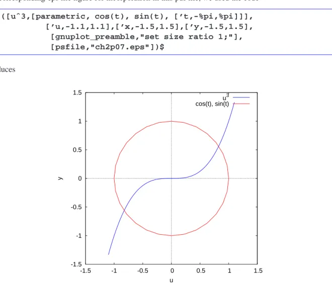
(%i5) plot2d ([uˆ3,[parametric, cos(t), sin(t), [’t,-%pi,%pi]]], [’u,-1.1,1.1],[’x,-1.5,1.5],[’y,-1.5,1.5],

[gnuplot_preamble,"set size ratio 1;"])$

in which[’u,-1.1,1.1]is required to determine the drawing range ofuˆ3, and we have added separate horizontal and vertical canvas control lists as well as the gnuplot preamble option to approximate a circle, since it is quicker than fiddling with the x and y ranges by hand.

To get the corresponding eps file figure for incorporation in this pdf file, we used the code plot2d ([uˆ3,[parametric, cos(t), sin(t), [’t,-%pi,%pi]]],

[’u,-1.1,1.1],[’x,-1.5,1.5],[’y,-1.5,1.5], [gnuplot_preamble,"set size ratio 1;"], [psfile,"ch2p07.eps"])$

which produces

-1.5 -1 -0.5 0 0.5 1 1.5

y

u

u³ cos(t), sin(t)

Figure 7: Combining an Explicit Expression with a Parametric Object in which the horizontal axis label (by default) isu.

(9)

We now add a few more options to make this combined plot look cleaner and brighter (more about some of these later).

(%i6) plot2d (

[ [parametric, cos(t), sin(t), [’t,-%pi,%pi],[nticks,200]],uˆ3], [’u,-1,1], [’x,-1.2,1.2] , [’y,-1.2,1.2],

[style, [lines,8]], [xlabel," "], [ylabel," "], [box,false], [axes, false],

[legend,false],[gnuplot_preamble,"set size ratio 1;"])$

and the corresponding eps file (with[lines,20]for increased line width) produces:

Figure 8: Drawing ofu³Over a Circle

The default value of nticks inside plot2d is29, and using[nticks, 200]yields a much smoother parametric curve.

2.1.4 Line Width and Color Controls

Each element to be included in the plot can have a separate [ lines, nlw, nlc ] entry in the style option list, with nlw determining the line width and nlc determining the line color. The default value of nlw is1, a very thin weak line. The use of nlw = 5 creates a strong wider line.

The default color choices (if you don’t provide a specific vlue ofnlc) consist of a rotating color scheme which starts with nlc = 1 (blue) and then progresses through nlc = 6 (cyan = greenish-blue) and then repeats.

(10)

You will see the colors with the associated values of nlc, using the following code which draws a set of vertical lines in various colors (a version of a histogram). This code also shows an example of using discrete list objects (to draw straight lines), and the use of various options available. You should run this code with your own hardware-software setup, to see what the defaultplot2dcolors are with your system.

(%i1) plot2d(

[ [discrete,[[0,0],[0,5]]], [discrete,[[2,0],[2,5]]], [discrete,[[4,0],[4,5]]],[discrete,[[6,0],[6,5]]], [discrete,[[8,0],[8,5]]],[discrete,[[10,0],[10,5]]], [discrete,[[12,0],[12,5]]],[discrete,[[14,0],[14,5]]] ], [style, [lines,6,0],[lines,6,1],[lines,6,2],

[lines,6,3],[lines,6,4],[lines,6,5],[lines,6,6], [lines,6,7]],

[x,-2,20], [y,-2,8],

[legend,"0","1","2","3","4","5","6","7"], [xlabel," "], [ylabel," "],

[box,false],[axes,false])$

Note that none of the objects being drawn are expressions or functions, so a draw parameter range list is not only not necessary but would make no sense, and that the optional horizontal canvas width control list above is[’x,-2,20].

The interactive gnuplot plot2d colors available on a Windows XP system (using XMaxima with Maxima ver. 5.31) thus are: 0 = cyan, 1 = blue, 2 = red, 3 = green, 4 = majenta, 5 = black, 6 = cyan, 7 = blue, 8 = red, ...

Adding the element [psfile,"c:/work2/ztest2.eps"]to the above plot2d code produces the figure displayed here:

0 1 2 3 4 5 6 7

Figure 9: Cyclic plot2d Colors with a Windows XP System

(11)

For a simple example which uses color and line width controls, we plot the expressionsuˆ2anduˆ3on the same canvas, using lines in black and red colors, and add a height control list, which has the syntax [’y, ymin, ymax].

(%i2) plot2d( [uˆ2,uˆ3],[’u,0,2], [’x, -.2, 2.5], [style, [lines,5,5],[lines,5,2]],

[’y,-1,4] )$

plot2d: some values were clipped.

The plot2d warning should not be of concern here.

The width and height control list parameters have been chosen to make it easy to see where the two curves cross for positive u. If you move the cursor over the crossing point, you can read off the coordinates from the cursor position printout in the lower left corner of the plot window. This produces the plot:

-1 0 1 2 3 4

0 0.5 1 1.5 2 2.5

y

u

u² u³

Figure 10: Black and Red Curves

2.1.5 Discrete Data Plots: Point Size, Color, and Type Control

We have seen some simple parametric plot examples above. Here we make a more elaborate plot which includes discrete data points which locate on the curve special places, with information on the key legend about those special points. The actual parametric curve color is chosen to be black (5) with some thickness (4), using [lines,4,5]

in thestylelist. We force large size points with special color choices, using the maximum amount of control in the [points, nsize, ncolor, ntype]style assignments.

(%i1) obj_list : [ [parametric, 2*cos(t),tˆ2,[’t,0,2*%pi]],

[discrete,[[2,0]]],[discrete,[[0,(%pi/2)ˆ2]]], [discrete,[[-2,%piˆ2]]],[discrete,[[0,(3*%pi/2)ˆ2]]] ]$

(%i2) style_list : [style, [lines,4,5],[points,5,1,1],[points,5,2,1], [points,5,3,1],[points,5,4,1]]$

(%i3) legend_list : [legend, " ","t = 0","t = pi/2","t = pi",

" t = 3*pi/2"]$

(%i4) plot2d( obj_list, [’x,-3,4], [’y,-1,40],style_list, [xlabel,"X = 2 cos( t ), Y = t ˆ2 "],

[ylabel, " "] ,legend_list )$

(12)

This produces the plot:

0 5 10 15 20 25 30 35 40

-3 -2 -1 0 1 2 3 4

X = 2 cos( t ), Y = t ²

t = 0 t = pi/2 t = pi t = 3*pi/2

Figure 11: Parametric Plot with Discrete Points

The points style option has any of the following forms:[points], or[points, point_size], or

[points, point_size, point_color], or[points, point_size, point_color, point_type], in order of increasing control.

The defaultpoint colorsare the same cyclic colors used by the lines style. The defaultpoint typeis a cyclic order starting with 1 = filled circle , then continuing 2 = open circle, 3 = plus sign, 4 = diagonal crossed lines as capital X, 5 = star, 6 = filled square, 7 = open square, 8 = filled triangle point up, 9 = open triangle point up, 10 = filled triangle point down, 11 = open triangle point down 12 = filled diamond, 13 = open diamond = 0, 14 = filled circle, which is the same as 1, and repeating the same cycle. Thus if you use[points,5]you will get good size points, and both the color and shape will cycle through the default order. If you use[points,5,2]you will force a red color but the shape will depend on the contents and order of the rest of the objects list.

You can see the default points cycle through both colors and shapes with the code:

plot2d([ [discrete,[[0,.5]]],[discrete,[[0.1,.5]]],

[discrete,[[0.2,.5]]],[discrete,[[0.3,.5]]], [discrete,[[0.4,.5]]],[discrete,[[0.5,.5]]],

[discrete,[[0.6,.5]]],[discrete,[[0.7,.5]]], [discrete,[[0,0]]],[discrete,[[0.1,0]]], [discrete,[[0.2,0]]],[discrete,[[0.3,0]]], [discrete,[[0.4,0]]],[discrete,[[0.5,0]]], [discrete,[[0.6,0]]],[discrete,[[0.7,0]]] ],

(13)

[style,[points,5]],[xlabel,""],[ylabel,""], [’x,-0.2,1],[’y,-0.2,0.7],

[box,false],[axes,false],[legend,false])$

which will produce something like

Figure 12: default point colors and styles, 1-8, then 9-16

You can also experiment with one shape at a time by defining a function dopt(n)which selects the shape with the integernand leaves the color blue:

dopt(n) := plot2d ([discrete,[[0,0]]],[style,[points,15,1,n]], [box,false],[axes,false],[legend,false])$

Next we combine a list of twelve (x,y) pairs of points with the key word discrete to form a discrete object type for plot2d, and then look at the data points without adding the optional canvas width control. Note that using only one discrete list for all the points results in all data points being displayed with the same size, color and shape.

(%i5) data_list : [discrete,

[ [1.1,-0.9],[1.45,-1],[1.56,0.3],[1.88,2], [1.98,3.67],[2.32,2.6],[2.58,1.14], [2.74,-1.5],[3,-0.8],[3.3,1.1],

[3.65,0.8],[3.72,-2.9] ] ]$

(%i6) plot2d( data_list, [style,[points]])$

(14)

This produces the plot

-3 -2 -1 0 1 2 3 4

1 1.5 2 2.5 3 3.5 4

y

x

Figure 13: Twelve Data Points with Same Size, Color, and Shape

We now combine the data points with a curve which is a possible fit to these data points over the draw parameter range [u, 1, 4].

(%i7) plot2d( [sin(u)*cos(3*u)*uˆ2, data_list], [’u,1,4], [’x,0,5],[’y,-10,8], [style,[lines,4,1],[points,4,2,1]])$

plot2d: some values were clipped.

which produces (approximately) the plot

-10 -8 -6 -4 -2 0 2 4 6 8

0 1 2 3 4 5

y

u

u²*sin(u)*cos(3*u) discrete2

Figure 14: Curve Plus Data

(15)

2.1.6 More gnuplot preamble Options

Here is an example of using the gnuplot preamble options to add a grid, a title, and position the plot key at the bottom center of the canvas. Note the use of a semi-colon between successive gnuplot instructions.

(%i1) plot2d([ u*sin(u),cos(u)],[’u,-4,4] ,[’x,-8,8], [style,[lines,5]],

[gnuplot_preamble,"set grid; set key bottom center;

set title ’Two Functions’;"])$

which produces (approximately) the plot

-3.5 -3 -2.5 -2 -1.5 -1 -0.5 0 0.5 1 1.5 2

-8 -6 -4 -2 0 2 4 6 8

u

Two Functions

u*sin(u) cos(u)

Figure 15: Using the gnuplot preamble Option

Another option you can use isset zeroaxis lw 5;to get more prominentxandyaxes. Another example of a key location would beset key top left;. We have also previously used set size ratio 1;to get a “rounder”

circle.

(16)

2.1.7 Creating Various Kinds of Graphics Files Using plot2d

The first method of exportingplot2ddrawings as special graphics files is to have the plot drawn in the Gnuplot window (either the XMaxima route, or usingwxplot2drather thanplot2dif you are using wxmaxima). Then left-click the left-most Gnuplot icon near the top of the Gnuplot window (“copy the plot to clipboard”). Then open an application which accomodates the graphics format you desire, and paste the clipboard image into the application, and then use Save As, selecting the graphics type of save desired.

The second method of exportingplot2ddrawings as special graphics files is to use thegnuplot_termoption as part of yourplot2dcommand. If you do not add an additional option of the form (for example)

[gnuplot_out_file, "c:/k1/myname.ext"]

whereextis replaced by an appropriate graphics type extension, thenplot2dcreates a file with the namemaxplot.ext in your current working directory.

For example,

(%i1) plot2d (sin(u),[’u,0,%pi], [gnuplot_term,’jpeg])$

will create the graphics filemaxplot.jpeg, and a further commmand

(%i2) plot2d (cos(u),[’u,0,%pi], [gnuplot_term,’jpeg])$

will overwrite the previous filemaxplot.jpegto create the new graphics file for the plot ofcos. To provide a different name for different plots, you would write, for example,

(%i3) plot2d (cos(u),[’u,0,%pi],

[gnuplot_out_file,"c:/work2/mycos1.jpeg"], [gnuplot_term,’jpeg])$

If you do not supply the complete path, the file is written in the/binfolder of the Maxima program installation. Turning to other graphics file formats, and ignoring the naming option part,

(%i4) plot2d (sin(u),[’u,0,%pi], [gnuplot_term,’png])$

will createmaxplot.png.

(%i5) plot2d (sin(u),[’u,0,%pi], [gnuplot_term,’eps])$

will createmaxplot.eps.

(%i6) plot2d (sin(u),[’u,0,%pi], [gnuplot_term,’svg])$

will createmaxplot.svg(a “scalable vector graphics” file openable byinkscape).

(%i7) plot2d (sin(u),[’u,0,%pi], [gnuplot_term,’pdf])$

will createmaxplot.pdf, which will be the cleanest plot of the above cases.

(17)

2.1.8 Using qplot for Quick Plots of One or More Functions

The file qplot.mac is posted with Ch. 2 and contains a function called qplot which can be used for quick plotting of functions in place of plot2d.

The function qplot (qfor “quick”) accepts the default cyclic colors but always uses thicker lines than the plot2d default, adds more prominent x and y axes to the plot, and adds a grid (which can be switched off using the third from the left gnuplot icon). Here are some examples of use. (We include use with discrete lists only for completeness, since there is no way to get the points style with qplot.)

(%i1) load(qplot);

(%o1) c:/work2/qplot.mac

(%i2) qplot(sin(u),[’u,-%pi,%pi])$

(%i3) qplot(sin(u),[’u,-%pi,%pi],[’x,-4,4])$

(%i4) qplot(sin(u),[’u,-%pi,%pi],[’x,-4,4],[’y,-1.2,1.2])$

(%i5) qplot([sin(u),cos(u)],[’u,-%pi,%pi])$

(%i6) qplot([sin(u),cos(u)],[’u,-%pi,%pi],[’x,-4,4])$

(%i7) qplot([sin(u),cos(u)],[’u,-%pi,%pi],[’x,-4,4],[’y,-1.2,1.2])$

(%i8) qplot ([parametric, cos(t), sin(t), [’t,-%pi,%pi]], [’x,-2.1,2.1],[’y,-1.5,1.5])$

The last use involved only a parametric object, and the list[’x,-2.1,2.1]is interpreted as a horizontal canvas width control list based on the symbolx.

While viewing the resulting plot, use of the two-key commandAlt-Spacebar, which normally brings up a resizing menu, instead switches from the gnuplot figure to a raw gnuplot window. You can get back to the figure usingAlt-Tab, but the raw gnuplot window remains in the background. You should resize the figure window by clicking on the Maximize (or Restore) icon in the upper right-hand corner. Both the figure and the raw gnuplot window disappear when you close (using, sayAlt-F4, twice: once to close the figure window, and once to close the raw gnuplot window).

The next example includes both an expression depending on the parameteruand a parametric object depending on a parametert, so we must have a expression draw list of the form:[’u,umin,umax].

(%i9) qplot ([ uˆ3,

[parametric, cos(t), sin(t), [’t,-%pi,%pi]]], [’u,-1,1],[’x,-2.25,2.25],[’y,-1.5,1.5])$

Here is approximatedly the result with the author’s system:

-1.5 -1 -0.5 0 0.5 1 1.5

-2 -1.5 -1 -0.5 0 0.5 1 1.5 2

u

Figure 16: qplot example

(18)

To get the same plot usingplot2dfrom scratch requires the code:

plot2d([ uˆ3, [parametric, cos(t), sin(t), [’t,-%pi,%pi]]], [’u,-1,1],[’x,-2.25,2.25],[’y,-1.5,1.5], [style,[lines,5]], [nticks,100],

[gnuplot_preamble, "set grid; set zeroaxis lw 5;"], [legend,false],[ylabel, " "])$

Here are two discrete examples which draw vertical lines.

(%i10) qplot([discrete,[[0,-2],[0,2]]],[’x,-2,2],[’y,-4,4])$

(%i11) qplot( [ [discrete,[[-1,-2],[-1,2]]],

[discrete,[[1,-2],[1,2]]]],[’x,-2,2],[’y,-4,4])$

Here is the code (in qplot.mac) which defines the Maxima function qplot.

qplot ( exprlist, prange, [hvrange]) :=

block([optlist, plist],

optlist : [ [nticks,100], [legend, false],

[ylabel, " "], [gnuplot_preamble, "set grid; set zeroaxis lw 5;"] ], optlist : cons ( [style,[lines,5]], optlist ),

if length (hvrange) = 0 then plist : []

else plist : hvrange, plist : cons (prange,plist), plist : cons (exprlist,plist), plist : append ( plist, optlist ), apply (plot2d, plist ) )$

In this code, the third argument is an optional argument. The local plist accumulates the arguments to be passed to plot2d by use of cons and append, and is then passed to plot2d by the use of apply. The order of using cons makes sure that exprlist will be the first element, (and prange will be the second) seen by plot2d. In this example you can see several tools used for programming with lists.

Several choices have been made in the qplot code to get quick and uncluttered plots of one or more functions. One choice was to add a grid and strongerxand yaxis lines. Another choice was to eliminate the key legend by using the option [legend, false]. If you want a key legend to appear when plotting multiple functions, you should remove that option from the code and reload qplot.mac.

(19)

2.1.9 Plot of a Discontinuous Function

Here is an example of a definition and plot of a discontinous function.

(%i12) fs(x) := if x >= -1 and x <= 1 then 3/2 else 0$

(%i13) plot2d (fs(u),[’u,-2,2],[’x,-3,3],[’y,-.5,2], [style, [lines,5]],[ylabel,""],

[xlabel,""])$

which produces (approximately) the plot:

-0.5 0 0.5 1 1.5 2

-3 -2 -1 0 1 2 3

Figure 17: Plot of a Discontinuous Function or we can useqplot:

(%i14) load(qplot);

(%o14) c:/work2/qplot.mac

(%i15) qplot (fs(u),[’u,-2,2],[’x,-3,3],[’y,-.5,2],[xlabel,""])$

to get the same plot.

2.2 Working with Files Using the Package mfiles.mac

The chapter 2 package filemfiles.mac(which loadsmfiles1.lisp) has some Maxima tools for working with both text and data files. Both files are available on the author’s webpage. Unless you use your initialization file to automatically loadmfiles.macwhen you start or restart Maxima, you will need to do an explicit load to use these functions.

2.2.1 Check File Existence with file search or probe file

To check for the existence of a file, you can use the standard Maxima functionfile_searchor themfilespackage function probe_file(the latter is experimental and seems to work in a M.S. Windows version of Maxima). In the following, the file ztemp.txtexists in the current working directory (c:/work2/), and the fileytemp.txtdoes not exist in this work folder.

Both functions returnfalsewhen the file is not found. You need to supply the full file name including any extension, as a string.

The XMaxima output shown here usesdisplay2d:true(the default). If you use the non-default setting

(display2d:false), strings will appear surrounded by double-quotes, but unpleasant backslash escape characters\will appear in the output.

(20)

In the following, we have not yet loadedmfiles.mac.

(%i1) file_search ("ztemp.txt");

(%o1) c:/work2/ztemp.txt

(%i2) probe_file ("ztemp.txt");

(%o2) probe_file(ztemp.txt)

(%i3) load(mfiles);

(%o3) c:/work2/mfiles.mac

(%i4) probe_file ("ztemp.txt");

(%o4) false

(%i5) probe_file ("c:/work2/ztemp.txt");

(%i6) myf : mkp("ztemp.txt");

(%i7) probe_file (myf);

(%i8) file_search ("ztemp");

(%o8) false

(%i9) file_search ("ytemp.txt");

(%o9) false

Although the core Maxima functionfile_searchdoes not need the complete path (due to ourmaxima.initfile contents), our homemade functions, such asprobe_filedo need a complete path, due to recent changes in Maxima.

To ease the pain of typing the full path, you can use a function which we callmkp(“make path”) which we define in our maxima.init.macfile, whose contents are:

/* this is c:\Documents and Settings\Edwin Woollett\maxima\maxima-init.mac */

maxima_userdir: "c:/work2" $ maxima_tempdir : "c:/work2"$

file_search_maxima : append(["c:/work2/###.{mac,mc}"],file_search_maxima )$

file_search_lisp : append(["c:/work2/###.lisp"],file_search_lisp )$

bpath : "c:/work2/"$

mkp (_fname) := sconcat (bpath,_fname)$

We have used this function,mkpabove, to getprobe_fileto work. The string processing functionsconcatcreates a new string from two given strings (“string concatenation”):

(%i10) display2d:false$

(%i11) sconcat("a bc","xy z");

(%o11) "a bcxy z"

Note that we defined (in our maxima-init.mac file) a global variablebpath(“base of path” or “beginning of path”) instead of using the global variablemaxima_userdir. This makes it more convenient for the user to redefinebpath

“on the fly” (inside a maxima session) instead of opening and editingmaxima-init.mac, and restarting Maxima to have the changes take effect.

We see thatfile_searchis easier to use thanprobe_file.

2.2.2 Check for File Existence using ls or dir

Themfiles.macpackage functionslsanddiraccept the use of a wildcard pathname. Both functions are experimental and are not guaranteed to work with Maxima engines compiled with a Lisp version different from GCL (Gnu Common Lisp) (which is the Lisp version used for the Windows binary used by the author).

(21)

Again, you must use the full path, and can make use of themkpfunction as in the above examples. The last examples below refer to a folder different than the working folderc:/work2/.

(%i12) ls(mkp("*temp.txt"));

(%o12) [c:/work2/REPLACETEMP.TXT, c:/work2/temp.txt, c:/work2/ztemp.txt]

(%i13) ls("c:/work2/*temp.txt");

(%o13) [c:/work2/REPLACETEMP.TXT, c:/work2/temp.txt, c:/work2/ztemp.txt]

(%i14) dir(mkp("*temp.txt"));

(%o14) [REPLACETEMP.TXT, temp.txt, ztemp.txt]

(%i15) dir("c:/work2/*temp.txt");

(%o15) [REPLACETEMP.TXT, temp.txt, ztemp.txt]

(%i16) ls ("c:/work3/dirac.*");

(%o16) [c:/work3/dirac.mac, c:/work3/dirac.tex]

(%i17) dir ("c:/work3/dirac.*");

(%o17) [dirac.mac, dirac.tex]

2.2.3 Type of File, Number of Lines, Number of Characters

The text file lisp1w.txt is a file with Windows line ending control characters which has three lines of text and no blank lines.

(%i18) file_search("lisp1w.txt");

(%o18) c:/work2/lisp1w.txt

(%i19) file_lines("lisp1w.txt");

openr: file does not exist: lisp1w.txt

#0: file_lines(fnm=lisp1w.txt)(mfiles.mac line 637) -- an error. To debug this try: debugmode(true);

(%i20) file_lines(mkp("lisp1w.txt"));

(%o20) [3, 3]

(%i21) file_lines("c:/work2/lisp1w.txt");

(%o21) [3, 3]

The output of thefile_linesfunction returns the list

[number of non-blank lines, total number of lines].

(%i22) myf:mkp("lisp1w.txt");

(%o22) c:/work2/lisp1w.txt

(%i23) ftype(myf);

(%o23) windows

(%i24) file_length(myf);

(%o24) 131

(%i25) file_info(myf);

(%o25) [3, 3, windows, 131]

The function ftype (file type) returns either windows, unix, ormac depending on the nature of the “end of line chars”. The function file_lengthreturns the number of characters (“chars”) in the file, including the end of line chars. The functionfile_infocombines the line number info, the file type, and the number of characters into one list.

2.2.4 Print All or Some Lines of a File to the Console

For a small file the packge functionprint_file(file)is useful. For a larger file print_lines(file,start,end)is useful.

(%i26) print_file (myf)$

Lisp (or LISP) is a family of computer programming languages with a long history and a distinctive, fully parenthesized syntax.

(%i27) myf : mkp("lisp2.txt");

(%o27) c:/work2/lisp2.txt

(22)

(%i28) file_info(myf);

(%o28) [8, 8, windows, 504]

(%i29) print_lines(myf,3,5)$

parenthesized syntax. Originally specified in 1958, Lisp is the second-oldest high-level programming language in

widespread use today; only Fortran is older (by one year).

2.2.5 Rename a File using rename file

Themfiles.macpackage functionrename_file (oldname,newname)is an experimental function which works as follows in a Windows version of Maxima (again we must use the complete path):

(%i30) file_search("foo1.txt");

(%o30) false

(%i31) file_search("bar1.txt");

(%o31) c:/work2/bar1.txt

(%i32) rename_file(mkp("bar1.txt"),mkp("foo1.txt"));

(%o32) c:/work2/foo1.txt

(%o33) c:/work2/foo1.txt

(%o34) false

2.2.6 Delete a File with delete file

Themfiles.macpackage functiondelete_file (filename)does what its name implies:

(%o35) c:/work2/bar2.txt

(%i36) delete_file(mkp("bar2.txt"));

(%o36) done

(%o37) false

2.2.7 Copy a File using copy file

Themfiles.macpackage function copy_file(fsource,fdest)will preserve the file type, but will not warn you if you are over-writing a previous file name.

(%o38) false

(%i39) file_info(mkp("foo1.txt"));

(%o39) [3, 3, windows, 59]

(%i40) copy_file(mkp("foo1.txt"),mkp("foo2.txt"));

(%o40) c:/work2/foo2.txt

(%i41) file_info(mkp("foo2.txt"));

(%o41) [3, 3, windows, 59]

2.2.8 Change the File Type using file convert

Here, “file type” refers to the text file typesunix,windows, andmac, each distinguised by the use of different conven- tions in indicating the end of a text file line.

Syntax:file_convert(file, newtype)or file_convert (oldfile, newfile,newtype)

The acceptable values ofnewtypearewindows,unix, andmac.

(23)

For example, we can change a unix file to a windows file usingfile_convert(f,windows)which replaces the previous file, or we can change a unix file to a windows file with a new name usingfile_convert(fold,fnew,windows).

It is easy to check the end of line characters using the Notepad2 View menu. Notepad2 also easily lets you change the end of line characters, so writing Maxima code for this task is somewhat unneeded, though instructive as a coding challenge.

(%o42) c:/work2/bar1.txt

(%o43) c:/work2/bar2.txt

(%i44) print_file(mkp("bar1.txt"))$

This is line one.

This is line two.

This is line three.

(%i45) file_info(mkp("bar1.txt"));

(%o45) [3, 3, windows, 59]

(%i46) file_convert(mkp("bar1.txt"),mkp("bar11u.txt"),unix);

(%o46) c:/work2/bar11u.txt

(%i47) file_info(mkp("bar11u.txt"));

(%o47) [3, 3, unix, 56]

(%i48) print_file(mkp("bar2.txt"));

(%o48) c:/work2/bar2.txt

(%o49) [3, 3, windows, 59]

(%i50) file_convert(mkp("bar2.txt"),mac);

(%o50) c:/work2/bar2.txt

(%o51) [3, 3, mac, 56]

(%i52) print_file(mkp("bar2.txt"));

(%o52) c:/work2/bar2.txt

2.2.9 Breaking File Lines with pbreak lines or pbreak()

Four paragraphs of the Lisp entry from part of Paul Graham’s web site were copied into a text fileztemp.txt. In Notepad2, each paragraph was one long line.

Inside Maxima, we then used themfilespackage functionpbreak_lines (file,nmax)to break the lines (at a space) and print the results to the console screen of Xmaxima.

(%i53) file_info(mkp("ztemp.txt"));

(%o53) [7, 13, windows, 1082]

(%i54) print_lines(mkp("ztemp.txt"),1,1);

6. Programs composed of expressions. Lisp programs are trees ...[continues]

(%i55) pbreak_lines(mkp("ztemp.txt"),60)$

6. Programs composed of expressions. Lisp programs are trees of expressions, each of which returns a value. (In some Lisps expressions can return multiple values.) This is in contrast to Fortran and most succeeding languages, which distinguish between expressions and statements.

It was natural to have this distinction in Fortran because (not surprisingly in a language where the input format was punched cards) the language was line-oriented. You could not nest statements. And so while you needed expressions

(24)

for math to work, there was no point in making anything else return a value, because there could not be anything waiting for it.

This limitation went away with the arrival of

block-structured languages, but by then it was too late.

The distinction between expressions and statements was entrenched. It spread from Fortran into Algol and thence to both their descendants.

When a language is made entirely of expressions, you can compose expressions however you want. You can say either (using Arc syntax)

(if foo (= x 1) (= x 2)) or

(= x (if foo 1 2))

Once the line breaking text appears on the console screen, one can copy and paste into a text file for further use.

It is simpler to use the functionpbreak()which hasnmax = 72hardwired in the code, as well as the name

"ztemp.txt"; this could be used in the above example aspbreak(), and is easy to use since you don’t have to type either the text file name or the value ofnmax.

The package functionpbreak()uses the current definition ofbpathandmkp, as well as the file name"ztemp.txt".

(%i56) pbreak();

6. Programs composed of expressions. Lisp programs are trees of

expressions, each of which returns a value. (In some Lisps expressions can return multiple values.) This is in contrast to Fortran and most succeeding languages, which distinguish between expressions and statements.

It was natural to have this distinction in Fortran because (not surprisingly in a language where the input format was punched cards) the language was line-oriented. You could not nest statements. And so while you needed expressions for math to work, there was no point in making anything else return a value, because there could not be anything waiting for it.

This limitation went away with the arrival of block-structured languages, but by then it was too late. The distinction between

expressions and statements was entrenched. It spread from Fortran into Algol and thence to both their descendants.

When a language is made entirely of expressions, you can compose expressions however you want. You can say either (using Arc syntax) (if foo (= x 1) (= x 2))

or

(= x (if foo 1 2))

(%o56) done

(25)

Alternatively, one can employ themfilespackage functionbreak_file_lines (fold,fnew,nmax)to dump the folded lines into created filefnew.

(%i57) break_file_lines (mkp("ztemp.txt"),mkp("ztemp1.txt"),72);

(%o57) c:/work2/ztemp1.txt

(%i58) print_lines(mkp("ztemp1.txt"),1,2);

6. Programs composed of expressions. Lisp programs are trees of

expressions, each of which returns a value. (In some Lisps expressions

(%o58) c:/work2/ztemp1.txt

(%i59) file_info(mkp("ztemp.txt"));

(%o59) [7, 13, windows, 1082]

(%i60) file_info(mkp("ztemp1.txt"));

(%o60) [20, 26, windows, 1095]

2.2.10 Search Text Lines for Strings with search file the default two arg behavior:

search_file(filename, substring)

is to return line number and line text only for lines in whichsubstringis a distinct word, as defined by the package functionsword, used by the package functionwsearch.

Using the form

search_file (filename,substring,word) produces exactly the same as the two arg default mode above.

Using the form

search_file (filename,substring,all)

will return line numbers and line text for all lines in which the package functionssearchreturns an integer, ie., all lines in which the substring appears, regardless of being a distinct word.

The simplest syntaxsearch_file (file, search-string)is first demonstrated with two searches of the file ndata1.dat, which happens to be a purely text file.

(%i61) file_info (mkp("ndata1.dat"));

(%o61) [5, 9, windows, 336]

(%i62) print_file (mkp("ndata1.dat"))$

The calculation of the effective cross section is much simplified if only those collisions are considered for which the impact parameter is large, so that the field U is weak and the angles of deflection are small. The

calculation can be carried out in the laboratory system, and the center of mass frame need not be used.

(%i63) search_file (mkp("ndata1.dat"),"is")$

c:/work2/ndata1.dat

1 The calculation of the effective cross section is much simplified if only 3 those collisions are considered for which the impact parameter is large, so 5 that the field U is weak and the angles of deflection are small. The

(%i64) search_file (mkp("ndata1.dat"),"is much")$

1 The calculation of the effective cross section is much simplified if only

(26)

We next demonstrate all three possible syntax forms with a purely text filetext1.txt.

(%i65) file_info (mkp("text1.txt"));

(%o65) [5, 5, windows, 152]

(%i66) print_file (mkp("text1.txt"))$

is this line one? Yes, this is line one.

This might be line two.

Here is line three.

I insist that this be line four.

This is line five, isn’t it?

(%i67) search_file (mkp("text1.txt"),"is")$

c:/work2/text1.txt

1 is this line one? Yes, this is line one.

3 Here is line three.

5 This is line five, isn’t it?

(%i68) search_file (mkp("text1.txt"),"is",word)$

(%i69) search_file (mkp("text1.txt"),"is",all)$

2 This might be line two.

4 I insist that this be line four.

2.2.11 Search for a Text String in Multiple Files with search mfiles

The most general syntax is search_mfiles (file or path,string,options...)in which the options recognised areword, all, cs, ic, used in the same way as described above for search_file. The simplest syntax issearch_mfiles (file or path,string)which defaults to case sensitive (cs) and isolated word (word) as options. An example of over-riding the default behavior (csandword) would be

search_mfiles (file or path, string,ic, all)and the options args can be in either order.

First an example of searching one file in the working directory.

(%i2) print_file(mkp("text1.txt"))$

(%i3) search_mfiles(mkp("text1.txt"),"is")$

(%i4) search_mfiles(mkp("text1.txt"),"Is")$

(%i5)

(27)

Next we use a wildcard type file name for a search in the working directory.

(%i5) search_mfiles(mkp("ndata*.dat"),"is")$

Next we return to a search of the single filetext1.txt, but look for lines containing the string"is"whether or not it is an instance of an isolated word.

(%i6) search_mfiles(mkp("text1.txt"),"is",all)$

2 This might be line two.

4 I insist that this be line four.

We now usesearch_mfilesto look for a text string in a fileatext1.txtwhich is not in the current working directory.

(%i2) search_mfiles ("c:/work2/temp1/atext1.txt","is");

c:/work2/temp1/atext1.txt

2 Is this line two? Yes, this is line two.

6 This is line six, Isn’t it?

(%o2) done

If you want to search all files in the folderc:/work2/temp1, you use the syntax:

(%i3) search_mfiles ("c:/work2/temp1/","is")$

c:/work2/temp1/calc1news.txt

9 The organization of chapter six is then:

96 The Maxima output is the list of the vector curl components in the 98 a reminder to the user of what the current coordinate system is 102 Thus the syntax is based on lists and is similar to (although better 105 There is a separate function to change the current coordinate system.

112 plotderiv(..) which is useful for "automating" the plotting c:/work2/temp1/ndata1.dat

c:/work2/temp1/stavros-tricks.txt

34 Not a bug, but Maxima doesn’t know that the beta function is symmetric:

(28)

c:/work2/temp1/text1.txt

c:/work2/temp1/trigsimplification.txt

13 (1) Is there a Maxima command that indicates whether expr is a product of 76 > (1) Is there a Maxima command that indicates whether expr is a product of 91 Well, that is inherent in their definition. Trigreduce replaces all

94 is sin(x)*cos(x), since the individual terms are not products of trigs.

95 There is no built-in function which tries to find the smallest expression, 151 is better. If the user wants to expand the contents of sin to discover 153 is right that Maxima avoids potentially very expensive operations in c:/work2/temp1/wu-d.txt

1 As a dedicated windows xp user who is delighted to have windows binaries

3 all who are considering windows use that there is no problem with keeping previous

2.2.12 Replace Text in File with ftext replace

The simplest syntax ftext_replace(file,sold,snew)replaces distinct substrings sold(separate words) by snew.

The four arg syntaxftext_replace(file,sold,snew,word)does exactly the same thing.

The four arg syntax ftext_replace(file,sold,snew,all) instead replaces all substrings soldby snew, whether or not they are distinct words.

In all cases, the text file type (unix, windows, or mac) is preserved.

The package functionftext_replacecalls the package function

replace_file_text (fsource, fdest, sold,snew, optional-mode)which allows the replacement to occur in a newly created file with a namefdest.

(%i4) file_info(mkp("text1w.txt"));

(%o4) [5, 5, windows, 152]

(%i5) print_file(mkp("text1w.txt"));