Symmetries in Physics
FS 2019
Matthias R. Gaberdiel
Institute for Theoretical Physics ETH Z¨ urich
H¨ onggerberg, HIT K23.1 CH-8093 Z¨ urich
Email: gaberdiel@itp.phys.ethz.ch
Contents
1 Finite Groups 3
1.1 Definition and Basic Examples . . . 3
1.2 Representations . . . 4
1.3 Complete Reducibility . . . 7
1.4 Equivalence of Representations and Schur’s Lemma . . . 9
1.5 Characters . . . 11
1.6 The Projection Formula . . . 12
1.7 The group algebra . . . 16
1.8 Crystal-field splitting . . . 17
1.9 Classification of crystal classes . . . 21
2 The symmetric group and Young diagrams 24
2.1 Conjugacy classes and Young diagrams . . . 24
2.2 Frobenius formula . . . 28
2.3 Equivalent particles . . . 32
2.4 Braid group statistics . . . 34
3 Lie groups and Lie algebras 37 3.1 From the Lie group to the Lie algebra . . . 37
3.1.1 Representations . . . 39
3.2 Lie algebras . . . 40
3.2.1 Killing Form . . . 41
3.2.2 Complexification . . . 44
4 Complex simple Lie algebras — the case of su(2) 46 4.1 The complexification of su(2) . . . 46
4.2 The representation theory . . . 46
4.3 The Clebsch-Gordan series . . . 48
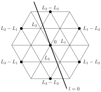
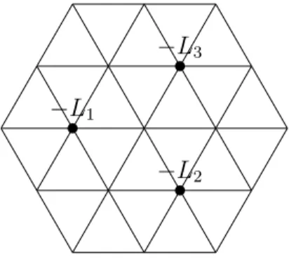
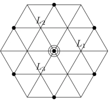
5 Complex simple Lie algebras — the case of su(3) 50 5.1 The complexification of su(3) and the Cartan-Weyl basis . . . 50
5.2 The general representation theory . . . 53
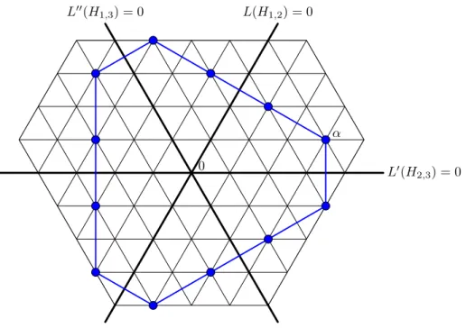
5.3 Explicit examples of sl(3,C) representations . . . 59
5.4 sl(3,C) representations in terms of Young diagrams . . . 63
6 General simple Lie algebras 68 6.1 The general analysis . . . 68
6.1.1 Representation theory . . . 69
6.2 The case of sl(N,C) . . . 71
6.3 Other simple Lie algebras . . . 74
1 Finite Groups
1.1 Definition and Basic Examples
Let us begin by reminding ourselves of the definition of a (finite) group. Consider a set Gof finitely (or infinitely) many elements, for which we define a law of combination that assigns to every ordered paira, b∈G a unique elementa·b ∈G. Here the products a·b and b·a need not be identical. We call G a group if
(i) G contains an element e ∈ G such that e·a = a·e = a for all a ∈ G. (e is then called the unit element or identity element.)
(ii) To every a∈G, there exists an inversea−1 ∈G so that a·a−1 =a−1·a=e.
(iii) The composition is associative, i.e.
(a·b)·c=a·(b·c) . (1.1.1) Simple examples of groups are the set of all integers Z, with the group operation being addition; or the set of all non-zero rationalsQ∗ or realsR∗ with the group operation being multiplication.
A more general class of examples is provided by the transformation groups. LetW be some set, and letG be the set of transformations
f :W →W (1.1.2)
that are one-to-one, i.e. x6=y implies f(x)6=f(y), and onto, i.e. for everyy ∈W, there exists anx∈W such thaty=f(x). Then G defines a group, where the group operation is composition, i.e.
(f ·g) (x) =f(g(x)) . (1.1.3) The identity element of G is the trivial transformation e(x) = x. Inverses exist since the transformations are one-to-one and onto, and the composition of maps is always associative. A prominent example of this kind are the symmetric groups Sn that are the transformation groups associated to Wn = {1, . . . , n}. The elements of Sn are the permutations, i.e. the invertible maps from {1, . . . , n} to itself. We may label them compactly as (heren = 7)
(1324)(5)(67) ←→
1 7→ 3 3 7→ 2 2 7→ 4 4 7→ 1 5 7→ 5 6 7→ 7 7 7→ 6
(1.1.4)
A group G is called abelian if a·b = b·a for all a, b ∈ G. For example, (Z,+) and (R∗,·) are abelian, while the permutation groupsSnwith n≥3 are not. A group is cyclic if it consists exactly of the powers of some element a, i.e. the group elements are
e ≡a0 ≡ap, a , a2, . . . , ap−1 (1.1.5) with the group operation
al·am =al+m , (1.1.6)
wherel+mis evaluated modp. Thiscyclic groupwill be denoted byCp in the following, and it also defines an abelian group.
Another important finite group is the dihedral group Dn, which is the symmetry group of a regularn-gon in the plane. Its elements are of the form
e≡dn, d , d2, . . . , dn−1 , s , sd , sd2, . . . , sdn−1 , (1.1.7) with the relations
s2 =dn=e , d−ks=sdk . (1.1.8) (Here d denotes the clockwise rotation of the n-gon, while s is the reflection around an axis.) Using (1.1.8) it is easy to see that the group elements of the form (1.1.7) close under the group operation.
For a finite groupG, the order |G| ofG is the number of elements in G. For example, for the cyclic group defined by (1.1.5), the order is|Cp|=p, while for the dihedral group we have |Dn|= 2n and for the symmetric group the order is
|Sn|=n!. (1.1.9)
1.2 Representations
A representation of a finite groupG on a finite-dimensional complex vector space V is a homomorphism
ρ:G→Aut(V) (1.2.1)
of G into the group of automorphisms of V. This is to say, to every a ∈ G, ρ(a) is an endomorphism of V that is invertible. Furthermore, the structure of G is respected by this map, i.e.
ρ(a·b) =ρ(a)◦ρ(b) ∀a, b∈G , (1.2.2) where ‘◦’ stands for composition of maps in Aut(V). In particular, it follows from this property that
ρ(e) =1 , (1.2.3)
the identity map fromV →V, and that
ρ(a−1) = (ρ(a))−1 . (1.2.4)
We say that such a mapρgives V the structure of aG-module; when there is little ambi- guity about the map ρ (and we are afraid, even sometimes when there is) we sometimes callV itself the representation of G. In this vein we will often suppress the symbolρ and writea·v oravfor (ρ(a))(v). The dimension ofV will sometimes be called the dimension of the representationρ.
If V has finite dimension, then upon introducing a basis in V, the linear transfor- mations can be described by non-singular n × n matrices. Thus a finite-dimensional representation ρ is an assignment of matrices ρ(a) for each group element a ∈ G such that (1.2.2) holds, where ‘◦’ on the right-hand-side stands for matrix multiplication. In this lecture we will always only consider finite-dimensional representations of groups.
As an example consider the symmetric group S3, that consists of the 6 permutations of the three symbols {1,2,3}. It is generated by the two transpositions
σ1 = (12)(3) , σ2 = (1)(23) (1.2.5)
subject to the relations that
σ12 =σ22 =e , σ1σ2σ1 =σ2σ1σ2 ; (1.2.6) the entire group then consists of the six group elements
e , σ1, σ2, σ1σ2, σ2σ1, σ1σ2σ1 . (1.2.7) It posseses a natural 3-dimensional representation, for which the group elements act as permutation matrices; thus the two generatorsσ1 and σ2 are represented by
ρ(σ1) =
0 1 0 1 0 0 0 0 1
, ρ(σ2) =
1 0 0 0 0 1 0 1 0
, (1.2.8)
etc. It is easy to see that this defines a representation of S3, i.e. that (1.2.2) is satisfied for all elements of S3. (This is just a consequence of the fact that the relations (1.2.6) are satisfied for ρ(σ1) and ρ(σ2).) Another representation of S3 is the 1-dimensional representation, the so-called alternating representation, defined by the determinant of these 3-dimensional matrices; it satisfies
ρd(σ1) = ρd(σ2) =ρd(σ1σ2σ1) =−1 , (1.2.9) as well as
ρd(σ1σ2) =ρd(σ2σ1) =ρd(e) = +1 . (1.2.10) Again, it is straightforward to check that ρd satisfies (1.2.2), now with ‘◦’ standing for regular multiplication.
A subrepresentationW is a vector subspaceW ⊆V wich is invariant under G, i.e.
which has the property that
ρ(a)w∈W ∀w∈W , a∈G . (1.2.11)
A representation V is called irreducible if V does not contain any subrepresentation other thanW =V orW ={0}. Otherwise the representation is called reducible.
Note that the above 3-dimensional representation (1.2.8) of S3 is notirreducible (i.e.
it is reducible). In particular, it contains the 1-dimensional subrepresentation
W =he1+e2+e3i . (1.2.12)
Indeed, it is easy to see that ρ(a)(e1 +e2+e3) = (e1+e2 +e3), i.e. that ρW(a) = 1 for alla ∈S3. This representation is therefore called thetrivial representation; obviously the trivial representation withρ(a)≡1 for all a∈G exists for every groupG.
IfV and W are representations ofG, the direct sum V ⊕W is also a representation ofG, where the action of Gis defined by
ρ=ρV ⊕ρW . (1.2.13)
Similarly, if V and W are representations of G, their tensor product V ⊗W is also a representation of G. Recall that if ei, i = 1, . . . , n and fj, j = 1, . . . , m are basis vectors forV and W, respectively, then a basis for V ⊗W is described by the pairs
ei ⊗fj , i∈ {1, . . . , n}, j ∈ {1, . . . , m} . (1.2.14) (Thus the tensor product V ⊗W has dimension dim(V) dim(W).) The tensor product representation is then defined by
a(v⊗w) = (a·v)⊗(a·w) ∀a∈G , v ∈V , w ∈W . (1.2.15) It is immediate that this defines a representation ofG.
Finally, if V is a representation of G, then also the dual vector space V∗ is a G- representation. In order to define the G-action on V∗ we use as a guiding principle that the natural pairing h·,·ibetween V∗ and V should be invariant under G, i.e. that
hρ∗(a)(v∗), ρ(a)(v)i=hv∗, vi , (1.2.16) where a ∈G, v ∈ V and v∗ ∈ V∗ are arbitrary. By rewriting this condition, replacing v byρ(a−1)v, we obtain the defining relation for ρ∗(a)
hρ∗(a)(v∗), vi=hv∗, ρ(a−1)vi . (1.2.17) Note that combining the definition of the dual and the tensor product then also allows us to make
Hom(V, W)∼=V∗⊗W (1.2.18)
into aG-representation, provided thatV andW areG-representations. (Here Hom(V, W) is the space of vector space homomorphisms fromV toW.) More explicitly, on the vector space homomorphismsϕ:V →W the G-action is defined by
(aϕ) (v) = a ϕ(a−1v). (1.2.19)
1.3 Complete Reducibility
As we have seen above, there are many different representations of a finite group. Before we begin our attempt to classify them we should try to simplify life by restricting our search somewhat. Specifically, we have seen that representations of G can be built up out of other representations by linear algebraic operations, most simply by taking the direct sum. We should focus then on representations that are ‘atomic’ with respect to this operation, i.e. that cannot be expressed as a direct sum of others; the usual term for such a representation is indecomposable. Happily, the situation is as nice as it could possibly be: a representation is atomic in this sense if and only if it is irreducible, i.e.
contains no proper subpresentation; and every representation is equivalent to the direct sum of irreducibles, in a suitable sense uniquely so. The key to all of this is the following:
Proposition: IfW is a subrepresentation of a representationV of a finite groupG, then there is a complementary invariant subspace W0 of V so thatV =W ⊕W0.
Proof: One simple way to prove this is the following. We define a positive definite hermitian inner producth·,·i onV which is preserved by each a∈G via
hv, wi ≡X
a∈G
hav, awi0 , (1.3.1)
whereh·,·i0 is any hermitian inner product on V. Recall that a hermitian inner product onV is an inner product satisfying
hv, wi=hw, vi∗ (1.3.2) as well as
hv, vi ≥0 , (1.3.3)
with equality if and only if v = 0 in V. On any n-dimensional complex vector space such an inner product exists. Ifh·,·i0 is an hermitian inner product onV, then so is h·,·i defined by (1.3.1). Furthermore,h·,·iis then invariant under the action of G, i.e. we have hv, wi=hbv, bwi for any b∈G, v, w∈V. (1.3.4) (This last statement simply follows from the fact that
hbv, bwi=X
a∈G
habv, abwi0 = X
a0∈G
ha0v, a0wi0 =hv, wi , (1.3.5) where in the middle step we have relabelled the sum overa by a sum over a0 =ab— as a runs over the whole groupG, so does a0, since the map froma 7→a0 is one-to-one with inverse a=a0b−1.)
Now with respect to the invariant hermitian inner producth·,·i we define the orthog- onal complement of W by
W⊥:={u∈V :hu, wi= 0, ∀w∈W} . (1.3.6)
Since the hermitian inner product is non-degenerate, we have
V =W ⊕W⊥ , (1.3.7)
i.e. the intersection of W and W⊥ is just the zero vector. Thus W⊥ plays the role of W0 in the proposition.
Finally, we observe that W⊥ also defines a subrepresentation ofV; to see this we only need to show thatau ∈W⊥ for any a∈G and u∈W⊥. But since
hw, aui=ha−1w, ui= 0 (1.3.8) for anyw∈W, this is the case, and we have shown that W⊥ is a suberpresentation of V. Note that by induction, this result implies that any (finite-dimensional) representation of a finite groupG is completely reducible, i.e. that it can be written as a direct sum of irreducible representations. As we shall see also compact continuous groups have this property — in fact the proof is fairly analogous since we can simply replace the sum over the group elements in (1.3.1) by an integral, using the invariant Haar measure of the compact group. However, there are also (infinite) groups for which complete reducibility does not hold. For example, for the group (Z,+) the 2−dimensional representation
n7→
1 n 0 1
(1.3.9) leaves the 1-dimensional subspace spanned bye1 invariant. However, there is no comple- mentary subspace that would also be invariant under the action of the group, and hence the above representation is reducible but indecomposable, i.e. it cannot be written as a direct sum of two 1-dimensional representations. However, for the remainder of these lectures we shall always consider groups whose representations are completely reducible.
For the example of the 3-dimensional representation ρ from (1.2.8), we have seen above, see eq. (1.2.12), there it contains a one-dimensional subrepresentation W. With respect to the standard inner product, the orthogonal complement ofW is then generated by
V ≡W⊥ =hf1 = (1,−1,0), f2 = (0,1,−1)i . (1.3.10) One easily confirms that the two generators in (1.2.8) act as
ρ(σ1)f1 =−f1 , ρ(σ1)f2 =f1+f2 , (1.3.11) as well as
ρ(σ2)f1 =f1+f2 , ρ(σ2)f2 =−f2 , (1.3.12) i.e. the two generators are represented by the 2×2 matrices
ρ(σ1)V =
−1 1
0 1
, ρ(σ2)V =
1 0 1 −1
. (1.3.13)
Again, one easily confirms that these matrices satisfy (1.2.6), as they must. Furthermore, it is easy to see that W⊥ does not contain any invariant 1-dimensional subspace, and hence that it must be irreducible. Thus the 3-dimensional representation (1.2.8) is in fact a direct sum of the 1-dimensional representation W as well as the 2-dimensional representationV ≡W⊥. V is called the ‘standard’ representation.
1.4 Equivalence of Representations and Schur’s Lemma
For our example of S3 we have now found three irreducible representations: the trivial representationW (1.2.12), the representation by signs ρd defined by (1.2.9) and (1.2.10), as well as the representation W⊥ defined by (1.3.13). As we shall see later, these are in fact the only irreducible representations of S3. However, before we can explain this, we first need to understand when we should regard two representations as ‘being the same’.
We shall say that two representationsρ1 :G→V1 and ρ2 :G→V2 are equivalent (or
‘the same’) provided that there exists an invertible linear map (in particular, this therefore implies thatV1 and V2 have the same vector space dimension, n= dim(V1) = dim(V2))
T :V1 →V2 (1.4.1)
such that
T ◦ρ1(a) =ρ2(a)◦T , ∀a∈G , (1.4.2) i.e. thatρ1 =T−1◦ρ2◦T. In terms ofn×n matrices, this condition therefore means that the n×n matrices ρ1(a) and ρ2(a) are conjugate to one another for all a∈G, where the conjugating matrix T is independent of a. Note that for 1-dimensional representations, two representationsρ1 and ρ2 are equivalent if and only if ρ1(a) = ρ2(a) for all a∈G.
Now that we have understood when two representations are the same, we can explain in which sense the decomposition of a representation into irreducibles is unique. This is a consequence of
Schur’s Lemma: Let V and W be irreducible representations of G and T : V → W a G-module homomorphism, i.e. a linear map satisfying
T ◦ρV =ρW ◦T . (1.4.3)
Then
(i) Either T is an isomorphism or T = 0.
(ii) If V =W, thenT =λ·1 for some λ∈C. (Here 1 is the identity map.)
Proof: First we note that the kernel ofT is an invariant subspace ofV, since ifv ∈ker(T) then (1.4.3) implies that
T ρV(a) (v)
=ρW(a) T(v)
= 0 , (1.4.4)
i.e. ρV(a) (v) is also in the kernel of T. Similarly, the image of T is an invariant subspace ofW: ifw∈W is in the image of T, i.e. w=T(v), then
ρW(a) T(v)
=T ρV(a)(v)
(1.4.5) is also in the image of T. Since V is irreducible, it follows that either ker(T) = V — in which caseT ≡0 — or ker(T) ={0}, in which caseT is one-to-one. Similarly, since W is irreducible, either im(T) ={0} — in which case T ≡0 — or im(T) = W, i.e.T is onto.
Combining these two statements eitherT ≡ 0, or T is both one-to-one and onto, i.e. an isomorphism. This proves (i).
In order to prove (ii), we use thatT must have at least one eigenvalueλ∈C. But then T−λ·1has a non-zero kernel, and hence, since it is also a G-module homomorphism, by the argument of case (i), it follows thatT −λ·1 ≡0. This proves that T =λ·1, i.e. the statement (ii).
As we have seen above, any representation V can be completely decomposed into irreducibles, i.e. we can write
V =V1⊕n1⊕ · · · ⊕Vk⊕nk , (1.4.6) where the Vi are distinct irreducible representations, and theni denote the multiplicities with which these representations appear in the decomposition. Schur’s Lemma now im- plies that this decomposition is unique in the sense that the same factors and the same multiplicities always appear. In order to see this, let us assume that we can also write V as
V =W1⊕m1 ⊕ · · · ⊕Wl⊕ml , (1.4.7) whereWj are distinct irreducible representations, andmj denote the multiplicities of these representations. Then since the identity map 1 :V → V is a G-module homomorphism, i.e. satisfies (1.4.3), Schur’s Lemma implies that1must map the summand Vi⊕ni into the summand Wj⊕mj for which Wj ∼= Vi, and furthermore that the multiplicities must agree.
This proves the uniqueness of the decomposition (4.2.1).
As we will see below, each finite group G only has finitely many irreducible repre- sentations. Once these are known, we therefore know in effect, because of (4.2.1), the most general representation of the group G. Thus in the following we shall concentrate on classifying the irreducible representations. One very powerful statement that we will derive is that the dimensions of these irreducible representations satisfies the identity
|G|= X
R irrep
dim(R)2 . (1.4.8)
For example, for the case of S3, this is the identity
3! = 6 = 1 + 1 + 22 , (1.4.9)
showing that the three irreducible representations from above, two 1-dimensional rep- resentations and the two-dimensional standard representation V, are in fact the only irreducible representations ofS3.
1.5 Characters
There is a remarkably effective tool for understanding the representations of a finite groupG, called character theory. It is in effect a way of keeping track of the eigenvalues of the action of the group elements. Of course, specifying all eigenvalues of the action of each element of G would be unwieldy, but fortunately, this would also be redundant.
For example, if we know the eigenvalues {λi} of an element a ∈ G, we also know the eigenvalues of ak for any k — they are just {λki}. The key observation here is that it is enough to give, for example, the sum of the eigenvalues of each element a ∈ G since knowing the sums P
iλki is equivalent to knowing the eigenvalues {λi} themselves. This then motivates the definition of the character of a representation as follows.
If V is a representation of G, its character χV is the complex-valued function on the group defined by
χV(a) = Tr(a|V) , (1.5.1)
i.e. the trace ofa onV. Note that in particular, we have
χV(bab−1) =χV(a) , (1.5.2)
i.e. the characterχV is constant on the conjugacy classes ofG. (Recall that the conjugacy class [a] of a ∈ G consists of all group elements that are conjugate to a, i.e. that are of the form bab−1 for some b ∈ G. This relation defines an equivalence relation, and hence the group can be split up into disjoint conjugacy classes. Note that the conjugacy class of the identity element just consists of the identity element itself.) A function that does not depend on the representative of each conjugacy class is called aclass function. Note that for the conjugacy class of the identity we simply haveχV(e) = dim(V).
Suppose V and W are representations of G. Then we have
χV⊕W =χV +χW , χV⊗W =χV ·χW χV∗ =χV . (1.5.3) In order to understand these identities, we consider a fixed group element a ∈ G. Then for the action of a, V has the eigenvalues {λi} while W has the eigenvalues {µj}. Then the eigenvalues onV ⊕W and V ⊗W are {λi, µj}and {λi·µj}, respectively, from which the first two formulae follow. Similarly{λ−1i =λi}are the eigenvalues forg onV∗, where we have used that all eigenvalues are n’th roots of unity, with n the order of the group elementa; this proves the last identity.
As we have said before, the character of a representation of a group G is really a function on the set of conjugacy classes inG. This suggests expressing the basic informa- tion about the irreducible representations of a group G in the form of a character table.
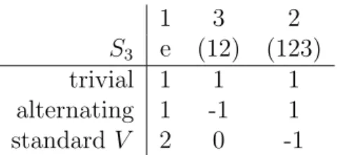
This is a table with the conjugacy classes [a] of G listed across the top, usually given by a representative a, with the number of elements in each conjugacy class over it; the irreducible representations V of G are listed on the left, and in the appropriate box the value of the characterχV on the conjugacy class [a] is given. For example, for the group S3 the character table takes the form given in Table 1.
1 3 2 S3 e (12) (123)
trivial 1 1 1
alternating 1 -1 1
standard V 2 0 -1
Table 1: Character Table of S3
Note that the conjugacy class (12) contains the three generators (12), (23) and (13), while the conjugacy class (123) contains the two generators (123) and (132). The traces in the trivial and alternating — the former is the representation W defined in (1.2.12), while the latter is the representation defined byρdin (1.2.9) and (1.2.10) — are immediate from the definition; the trace for (12) in V follows directly from (1.3.13), while that of (123) = (23)(12) =σ2σ1 or (132) = (12)(23) =σ1σ2 follows from
ρV(σ2σ1) =
−1 1
−1 0
, ρV(σ1σ2) =
0 −1 1 −1
. (1.5.4)
Note that, by (1.5.3), the character in the 3-dimensional representationρin (1.2.8) (that can be written as W ⊕V) is then
χρ(e) = 3 , χρ(12) = 1, χρ(123) = 0 (1.5.5) as one also directly verifies. In fact, we could have determined the decomposition ofρinto W ⊕V from this character identity since the three character functions are independent.
This is to say, if we make the ansatz
Vρ =n1(trivial) +n2(alternating) +n3V (1.5.6) then the right-hand-side implies that
χV(e) =n1 +n2+ 2n3 , χV(12) =n1−n2 , χV(123) =n1+n2−n3 . (1.5.7) So for the case at hand, we get the identities
n1+n2 + 2n3 = 3 , n1−n2 = 1 , n1+n2−n3 = 0 , (1.5.8) from which n1 = 1, n2 = 0 and n3 = 1 is the only solution. This basic idea will play an important role in the following.
1.6 The Projection Formula
We now want to make this more systematic, and in particular, determine the trivial factor in the decomposition of an arbitrary representation. Suppose V is a representation of G.
Then we define the invariant subspace ofV as
VG ={v ∈V :av=v ∀a ∈G} . (1.6.1)
We define the map
ϕ= 1
|G|
X
a∈G
a∈End(V) . (1.6.2)
Note that ϕ defines a G-module homomorphism, i.e. b◦ϕ = ϕ◦b for any b ∈ G; this follows simply from the fact
X
a∈G
a=X
a∈G
b−1ab= X
a0∈G
a0 , (1.6.3)
where we have defined a0 = b−1ab in the last step. Next we claim that ϕ defines the projection ofV ontoVG. First, we show that ϕ(V)⊂VG: let v =ϕ(w). Then we have
b ϕ(w) = 1
|G|
X
a∈G
baw = 1
|G|
X
a0∈G
a0w=ϕ(w) , (1.6.4) wherea0 =ba, thus showing ϕ(V)⊂VG. Conversely, suppose v ∈VG. Then
ϕ(v) = 1
|G|
X
a∈G
av = 1
|G|
X
a∈G
v =v , (1.6.5)
thus showing VG ⊂ ϕ(V). Hence we conclude that ϕ(V) = VG. Note that the last identity also implies thatϕ◦ϕ=ϕ.
We can use this method to determine explicitly the multiplicity with which the trivial representation appears in V; this number is just
n1 = dimVG= TrV(ϕ) = 1
|G|
X
a∈G
TrV(a) = 1
|G|
X
a∈G
χV(a). (1.6.6) For example, for the case of the 3-dimensional representation ρ in (1.2.8) (that can be written asW⊕W⊥) the multiplicity with which the trivial representation (that we called W) appears in ρ equals
n1 = 1 6
χρ(e) + 3χρ (12)
+ 2χρ (123)
= 1
6 3 + 3·1 + 2·0
= 1 . (1.6.7)
However, we can actually do much more with this idea. First we note that
Hom(V, W)G={G-module homomorphism from V toW} , (1.6.8) since the condition that ϕ : V → W is G-invariant means (see eq. (1.2.19)) that for all a∈G
a ϕ(a−1v) = ϕ(v) =⇒ ϕ◦a0 =a0◦ϕ (a0 =a−1) , (1.6.9) compare (1.4.3). Next we observe that if V is irreducible, then by the proof of Schur’s Lemma, ker(ϕ) is either 0 or V itself, and
dim Hom(V, W)G
=mV ≡multiplicity with whichV appears in W . (1.6.10)
On the other hand, we know that
Hom(V, W)∼=V∗ ⊗W , (1.6.11)
and thus we can apply the above trick to this tensor product. Using the character formula for the tensor product and the dual representation, see eq. (1.5.3), we therefore conclude that
mV = 1
|G|
X
a∈G
χV(a)·χW(a). (1.6.12)
Thus we can determine the multiplicity with which every irreducible representation ap- pears in a given representation using these character techniques. For example, for the above 3-dimensional representationρ of S3, see (1.2.8), we deduce from this that
n2 = 1 6
χa(e)χρ(e) + 3·χa (12)
χρ (12)
+ 2·χa (123)
χρ (123)
= 1
6
(1)(3) + 3·(−1)·1 + 2·(1)(0)
= 0 (1.6.13)
and
n3 = 1 6
χW⊥(e)χρ(e) + 3·χW⊥ (12)
χρ (12)
+ 2·χW⊥ (123)
χρ (123)
= 1
6
(2)(3) + 3·(0)·1 + 2·(−1)(0)
= 1 , (1.6.14)
in agreement with what we saw above.
Note that if W is also irreducible, we learn from this that the characters of the irre- ducible representations are orthonormal with respect to the hermitian inner product on the space of class functions defined by
(α, β) = 1
|G|
X
a∈G
α(a)β(a). (1.6.15)
For example, for the case of S3 above, this property can be directly read off from the character table, see Tab. 1, where the numbers over each conjugacy class tell us how many times to count entries in that column.
As a consequence it immediately follows that the number of irreducible representations of G is less than or equal to the number of conjugacy classes. In fact, we shall soon see that the number is always exactly equal, i.e. that there are no non-zero class functions that are orthogonal to all characters.
It is very instructive to apply these ideas to the regular representation of G, i.e. to the left-action ofG on itself. For the regular representation, the underlying vector space R has a basis {ea} labelled by the group elements a ∈ G, and the action of b ∈G on ea
equals
b(ea) =eba . (1.6.16)
This clearly defines a representation R of G of dimension dim(R) = |G|. It is clear by construction that the character ofR equals
χR(a) =
0 if a6=e
|G| if a=e. (1.6.17)
If we decomposeR into irreducibles as R=L
iVi⊕ni, then ni = 1
|G|
X
a∈G
χVi(a)χR(a) =χVi(e) = dim(Vi). (1.6.18) Thus we derive the desired relation between the size of the group and the dimensions of the irreducible representations,
|G|=X
i
dim(Vi)2 . (1.6.19)
It remains to show that there are no non-zero class functions that are orthogonal to all characters, i.e. that the number of irreducible representations equals the number of conjugacy classes ofG. To this end suppose that α:G→C is any function on the group G. Given any representation V of Gwe define the endomorphism of V
ϕα,V =X
a∈G
α(a)·a:V →V . (1.6.20)
We now claim thatϕα,V is a homomorphism of G-modules, i.e. satisfies
b◦ϕα,V =ϕα,V ◦b ∀ b∈G (1.6.21)
for all representationsV if and only if α is a class function, i.e. if
α(bab−1) =α(a) ∀ a, b∈G . (1.6.22) In order to see this let us write
(ϕα,V ◦b)(v) = X
a∈G
α(a)·a(bv)
= X
a∈G
α(bab−1)·bab−1(bv) [substitute a7→bab−1]
= X
a∈G
α(bab−1)·b(av). (1.6.23)
Now if α is a class function, α(bab−1) = α(a), then the last equation can be written as
bX
a∈G
α(a)·av
= (b◦ϕα,V)(v) . (1.6.24)
Conversely, suppose α is not a class function, i.e. there exist a0, b0 ∈ G such that α(b0a0b−10 ) 6=α(a0). We consider the regular representation of G, i.e. the representation ofG on itself by left-action, see eq. (1.6.16). For v =ee we then have
(ϕα,G◦b0)(ee) =X
a∈G
α(b0ab−10 )·eb0a 6=X
a∈G
α(a)·eb0a = (b0◦ϕα,G)(ee) , (1.6.25) where the inequality is a consequence of the fact that the coefficient of the basis vector eb0a0 is different between the two sides. This proves the converse direction.
This result now implies that the characters of the irreducible representations form an orthonormal basis for the space of class functions. To see this suppose that α is a class function that is orthonormal to all the characters of the irreducible representations, i.e.
X
a∈G
α(a)χV(a) = 0 (1.6.26)
for all (irreducible) V. (Note that since this is true for all representations, we may use χV∗ = χV to remove the complex conjugate from the second factor.) Let V be one of these irreducible representations, and consider again the endomorphism ϕα,V defined as above in eq. (1.6.20). Then by Schur’s Lemma ϕα,V = λ·1 for some λ ∈ C, and with n= dim(V) we have
λ = 1
nTrV(ϕα,V) = 1 n
X
a∈G
α(a)χV(a) = 0 . (1.6.27) Thusϕα,V = 0 or P
a∈Gα(a)·a = 0 on any irreducible representation V of G. But since any representation can be written as a direct sum of irreducibles, this statement is true on any representation, in particular the regular representation. But then, by a similar argument as above in eq. (1.6.25), it follows thatα≡0. This completes the proof.
1.7 The group algebra
There is an important notion that we have already dealt with implicitly, but not explicitly:
this is the group algebra CG associated to a finite group G. This is an object that, for all intents and purposes, can completely replace the groupGitself. Any statement about the representations ofG has an exact equivalent statement about the group algebra.
The underlying vector space of the group algebra of G is the vector space with basis {ea}corresponding to the different elementsa∈G, i.e. the underlying vector space of the regular representation. We define the algebra structure on this vector space simply by
ea·eb =eab . (1.7.1)
By a representation of the group algebra CG on a vector space V we mean simply an algebra homomorphism
CG→End(V) , (1.7.2)
i.e. a representation V of CG is the same thing as a left CG-module. Note that a repre- sentation ρ: G→ End(V) will extend, by linearity, to a map ˜ρ :CG →End(V) so that representations of CG correspond exactly to representations of G. The left CG-module given by CGitself corresponds to the regular representation.
If {Wi} are the irreducible representations of G, then we have seen that the regular representationR decomposes as
R=M
i
(Wi)⊕dim(Wi) . (1.7.3)
We can now refine this in terms of the group algebra as the statement that, as algebras, CG∼=M
i
End(Wi). (1.7.4)
To see this we recall that for any representation W of G, the map ρ : G → End(W) extends by linearity to a map CG → End(W). Applying this to each of the irreducible representationsWi gives us a canonical map
ϕ:CG→ M
i
End(Wi) . (1.7.5)
This map is injective since the representation on the regular representation is faithful, i.e.
different group elements act differently. Since both have dimensionP
(dimWi)2, the map is an isomorphism.
1.8 Crystal-field splitting
As an application of these techniques we consider the following physical problem which can be solved elegantly using group theoretic methods. (This analysis was pioneered by Bethe in the 1920s.)
When an atom or ion is located not in free space, but in a crystal, it is subjected to various inhomogeneous electric fields which destroy the isotropy of free space. In particular, the symmetry group is reduced from that of the full three-dimensional rotation group to some finite group of rotations through finite angles (and perhaps also reflections).
We shall discuss the representation theory of continuous groups (such as the three- dimensional rotation group) in later sections, but we recall for the moment that the energy spectrum of electrons in an atom (e.g. the hydrogen atom) are most conveniently described in terms of spherical harmonics. These are nothing but special families of functions that transform in irreducible representations of the rotation group. Indeed, as you learned in quantum mechanics, the set of spherical harmonics
Yl,m(θ, ϕ) , m=−l, . . . , l , (1.8.1) where l = 0,1, . . . is fixed, transform under rotations into one another and correspond to the irreducible representation Dl of the rotation group of dimension 2l + 1. Since
rotations change the value of m, this in particular implies that the energy spectrum of a rotationally symmetric problem such as the hydrogen atom can only depend onn (the additional quantum number characterising the radial behaviour) and l, but not on m. In fact, as you probably remember, for the case of the hydrogen atom, the energy spectrum is even independent ofl, but this is a sign of an even bigger underlying symmetry that is associated to the Runge-Lenz vector.
Let us consider the case of an ion in a crystal at a site where it is surrounded by a regular octahedron of negative ions; this is a reasonable approximation of the real situation in a large number of instances. The discrete symmetry group that maps the adjacent ions into one another contains then the octahedral groupO, i.e. the group of proper rotations that take a cube or a octahedron into itself. (The relation between the octahedron and the cube is that we can embed the octahedron into the cube so that the vertices of the octahedron sit at the face centers of the cube, while the face centers of the octahedron are in one-to-one correspondence with the vertices of the cube. Thus we may equivalently think of O as being the group of rotational symmetries of the cube.)
The rotational symmetries of the cube contain 24 elements: (i) for each of the 4 body diagonals, there are 2 non-trivial rotations, leading to 8 = 4·2 diagonal rotations; (ii) for each of the three axes through the face centers of opposite faces — we can naturally think of them as the x, y and z-axis — there are 3 non-trivial rotations, leading to 9 = 3·3 x, y, z rotations; (iii) finally for each of the 6 axes through the origin that are parallel to face diagonals there is one non-trivial 180-degree rotation, leading to 6 = 6·1 Altogether, and including the identity generator, we therefore have a group of 8 + 9 + 6 + 1 = 24 elements,|O|= 24.
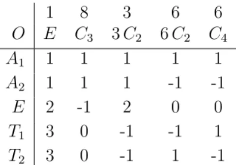
In terms of conjugacy classes, there is the conjugacy class of the identity E; the conjugacy class containing the order 3 rotations along the diagonalC3 — it contains all 8 such elements; the conjugacy classC4 of the order 4 rotations alongx, y, z — it contains all 6 such elements. In addition there are two conjugacy classes of order 2 elements, one associated to the order 2 rotations along thex, y, z axis — we shall denote it by 3C2 since it contains 3 elements — and one containing all 6 order two rotations of (iii) — this will be denoted by 6C2. The character table then has the form given in table 2, where the different representations have been labelled (following the usual convention in molecular physics)A1, A2, E, T1 and T2.
1 8 3 6 6
O E C3 3C2 6C2 C4
A1 1 1 1 1 1
A2 1 1 1 -1 -1
E 2 -1 2 0 0
T1 3 0 -1 -1 1
T2 3 0 -1 1 -1
Table 2: Character Table of O
Note that A1 is the identity representation, and that the different characters are or- thonormal with respect to the standard inner product on the space of class functions (1.6.15).
Now consider an electron with angular momentum quantum numberLwith respect to the usual 3-dimensional rotation group. The (2L+1) spherical harmonics that describe the different values forM all have degenerate energy eigenvalues in isotropic space. However, with respect to the smaller octahedral symmetry group, this irreducible representation of the rotation group will now not be irreducible, but will rather be a direct sum of irreducibleO-representations. Thus in the presence of the lattice, one should expect that the (2L+1)-fold degeneracy of the eigenstate will be lifted according to the decomposition into O-representations. (The states that sit in the same irreducible O-representation will continue to have degenerate energy eigenvalues, but for those that sit in different irreducible O-representations this will not generically be the case.) Thus without doing any real calculation, we can make a qualitative prediction for how the degeneracies will lift in the presence of the crystal!
In order to understand this more concretely, all we have to do is to understand how the irreducibleDLrepresentation decomposes with respect to theO-action. In fact, given our results above, it is enough to know the character of the various conjugacy classes of O in theDL representation. Recall that in the representation DL, a rotation by an angle α leads to the trace
χL(α) =
L
X
M=−L
eiM α =e−iLα
2L
X
m=0
eimα =e−iLα1−ei(2L+1)α
1−eiα (1.8.2)
= ei(L+12)α−e−i(L+12)α
eiα2 −e−iα2 (1.8.3)
= sin (L+12)α)
sin(α2) . (1.8.4)
Since the different conjugacy classes of O all correspond to rotations we therefore find
χL(E) = 2L+ 1 (1.8.5)
χL(C3) = χL(2π3 ) = sin (L+12)2π3 sin(π3) =
1 L= 0,3, . . . 0 L= 1,4, . . .
−1 L= 2,5, . . .
(1.8.6)
χL(C2) = χL(π) = sin (L+12)π
sin(π2) = (−1)L (1.8.7)
χL(C4) = χL(π2) = sin (L+ 12)π2 sin(π4) =
1 L= 0,1,4,5, . . .
−1 L= 2,3,6,7, . . . , (1.8.8) where the characters in the two C2 conjugacy classes are the same — the corresponding rotations are in different conjugacy classes of O, but in the same conjugacy class of the full rotation group.
Now we have all the information to determine the decomposition ofDLinto irreducible O-representations using (1.6.12). For the first few cases we find explicitly
D0 =A1
D1 =T1 3→3
D2 =E⊕T2 5→2 + 3
D3 =A2⊕T1⊕T2 7→1 + 3 + 3 D4 =A1⊕E⊕T1⊕T2 9→1 + 2 + 3 + 3 ,
(1.8.9)
as one easily verifies by comparing characters. So for example, this implies that the degeneracy of the 3 states with angular momentum number L = 1 is not lifted by the crystal, whereas the degeneracy of the 5 states with angular momentum numberL= 2 is lifted into a two-fold and a three-fold degenerate level, etc.
In most crystals there are at least small departures from cubic symmetry at the lattice site of a magnetic ion. We can take these (smaller) effects into account by considering now the breaking of the O-representations into representations of the smaller symmetry group that are still respected by the deformed lattice. For example, let us assume that the octahedron of ions producing the crystal field is distorted by an elongation along one of the threefold axes. This reduces the rotational symmetry to the dihedral group D3 that is a subgroup of O. The groupD3 consists of 6 elements that sit in three conjugacy classes: the identity element (that is a conjugacy class by itself); the conjugacy class of order 3 elements (that contains 2 elements, namely d and d2 in the notation of (1.1.7));
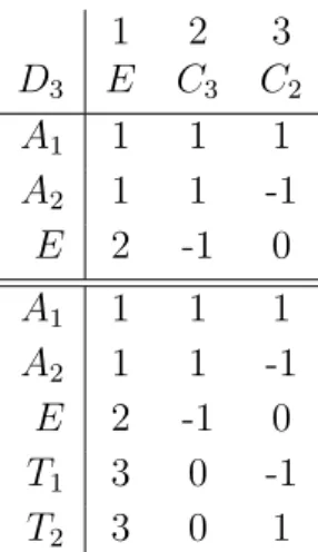
as well as the conjugacy class of order 2 elements (that contains 3 elements, namelys,sd and sd2, again in the notation of (1.1.7)). Its character table as well as the characters of the irreducible O representations is given in table 3
1 2 3
D3 E C3 C2
A1 1 1 1
A2 1 1 -1
E 2 -1 0
A1 1 1 1
A2 1 1 -1
E 2 -1 0
T1 3 0 -1 T2 3 0 1
Table 3: Character Table ofD3 (upper block). The representations below the double line refer to the O-representations.
We conclude from this that we have the branching rules from O to D3 given by A1 =A1
A2 =A2 E =E
T1 =A2⊕E 3→1 + 2 T2 =A1⊕E 3→1 + 2 ,
(1.8.10)
i.e. theO-representationsA1,A2 andE are irreducible with respect toD3 (where they are denoted by the same symbol), whereas the two 3-dimensionalO-representationsT1andT2 decompose into a direct sum of a 1-dimensional and a 2-dimensional D3 representation.
As a consequence, while the degeneracy of the 3 states with angular momentum num- berL= 1 is not lifted by the perfect crystal, a small elongation along one of the threefold axes will induce a small splitting of 3→1 + 2. Similarly, the 5 states atL= 2 are split by the perfect crystal into a two-fold and a three-fold degenerate level; the small elongation will not lift the degeneracy of the two-fold level, but will split the three-fold level further as 3→1 + 2, etc.
This example shows how simple group theoretic methods allow us to gain important structural insight into the qualitative features of a problem without doing actual detailed calculations. This is one of the central themes of this course.
1.9 Classification of crystal classes
In the above example we have considered two lattices, the perfect cubic lattice whose symmetry group (fixing a lattice point) contained the octahedral groupO, as well as the deformed lattice whose symmetry group was the dihedral group D3. One may ask what other groups may arise as symmetry groups of 3-dimensional lattices, and in fact one can show that there are only 32 possible symmetry groups. Accordingly, the lattices can be classified into 32 so-called crystal classes.
While we shall not attempt to prove this classification in detail, we want to under- stand at least schematically what sorts of groups can arise, and why there are only 32 possibilities. First of all, we are only interested in the point groups of the lattice, i.e.
in the group of lattice symmetries that fix a specific lattice point which we may take to be the origin. The corresponding group elements can then be thought of as real 3×3 matrices. Furthermore, since the angles between the various lattice vectors are preserved, these 3×3 matrices must be orthogonal.
The first step of the classification consists of finding all finite subgroups of O(3), the group of orthogonal 3×3 matrices. The relevant subgroups can be classified; they are either pure rotation groups, i.e. only contain elements in SO(3) with determinant +1, or contain also some reflections. The possible pure rotation groups are
• the cyclic group Cg of order g, consisting of g proper rotations about a fixed axis;
• the dihedral groupDh of order 2hconsisting of all proper rotations carrying a plane regular h-sided polygon in space onto itself: these include the h proper rotations about an axis perpendicular to the plane, together with h proper 180 degree rota- tions about the symmetry axes in the plane of the polygon;1
• the tetrahedral group T of order 12, consisting of the proper rotations carrying a regular tetahedron onto itself;
• the octahedral group O or order 24, consisting of the proper rotations carrying a cube into itself;
• the icosahedral group I of order 60, consisting of the proper rotations carrying a regular icosahedron into itself. (This group is isomorphic to the alternating group A5.)
In all of these cases it is also possible to adjoin some reflection symmetries to these pure rotation groups, but in each case there are at most two ways of doing so. But since the order of the group elements for the first two classes of groups, Cg and Dh is not yet constrained, at this stage we still have an infinite list of possible symmetry groups.
To cut this list down to finite size, the following observation is crucial. So far we have studied the possible finite orthogonal symmetry groups of O(3), but we haven’t yet used that this must map an actual lattice into itself. For example, in a suitable orthonormal basis the rotations in Cg or Dh are of the form
R(ϕ) =
1 0 0
0 cosϕ −sinϕ 0 sinϕ cosϕ
. (1.9.11)
However, if this transformation maps the lattice to itself, it must map each basis vector of the lattice to a linear combination (with integer coefficients) of lattice basis vectors.
Thus in the lattice basis (that is typically not orthonormal) the matrix R(ϕ) must be described by a matrix with integer entries. The lattice basis is related, by a change of coordinates, to the above orthonormal basis, and hence, for example, the trace of the matrix is independent of which basis is being used. But this then implies that the trace of R(ϕ) must be an integer since it equals an integer in the lattice basis. On the other hand, we have explicitly
Tr R(ϕ)
= 1 + 2 cosϕ . (1.9.12)
In order for this to be an integer, the possible angles are therefore ϕ=±π
3 , ±π
2 , ±2π
3 ,±π . (1.9.13)
1From the 2-dimensional viewpoint of the plane containing the polygon, this group also includes the
‘reflection’ s, see (1.1.7), but from the 3-dimensional viewpoint that is relevant here, this reflection is described by a 180 degree rotation about an axis in the plane of the polygon.
Thus we conclude that the possible orders of rotations are 1, 2, 3, 4 or 6, and thus the possible groupsCg and Dh that can appear have
h, g ∈ {1,2,3,4,6} . (1.9.14) It is then clear that the complete list of symmetry groups is finite, and a detailed analysis leads to the 32 cases mentioned before. (A more comprehensive discussion may be found in [FS, Chapter 8.2 & 8.3] or [T, Chapter 4.2].)
2 The symmetric group and Young diagrams
For some aspects of Lie theory (that will form the center of attention of the second half of this course) the symmetric group plays an important role. We therefore want to understand its representation theory in some detail.
2.1 Conjugacy classes and Young diagrams
Recall that Sn is the group of 1-to-1 transformations of the set {1, . . . , n}. As we have seen before, each element ofSn may be described in terms of cycles, describing the orbits of the different elements of{1, . . . , n}. It is not difficult to see that the conjugacy classes ofSnare then labelled by the cycle shapes, i.e. by the specification of how many cycles of which length the permutation has. For example, for the permutation described in (1.1.4), we have
(1324)(5)(67) ←→ cycle shape 112141, (2.1.1) i.e. there is one cycle of length 1, 2 and 4 each. We shall denote the conjugacy classes by Ci, wherei is a multiindex
i= (i1, i2 . . . , in) , (2.1.2) with ij denoting the number of cycles of length j. So for the above example we have i= (1,1,0,1,0,0,0). Note that we have the identity
n=
n
X
j=1
j ij , (2.1.3)
i.e. the cycle shapes define apartitionofninto positive integers. The number of conjugacy classes of Sn is therefore equal to the number of partitions p(n) of n. Its generating function equals
∞
X
n=0
p(n)tn =
∞
Y
m=1
1 1−tm
= (1 +t+t2+t3+· · ·)(1 +t2+t4+· · ·)(1 +t3+t6+t9+· · ·)· · ·
= 1 +t+ 2t2+ 3t3 + 5t4+ 7t5+· · · , (2.1.4) i.e. S2 has 2 conjugacy classes, S3 has 3 conjugacy classes, etc. (This last statement is obviously in agreement with what we saw explicitly above, see table 1.) The above generating function has interesting arithmetic properties and has been carefully studied;
for example, the partition numbers grow asymptotically as p(n)∼eπ
√2n
3 . (2.1.5)
We can describe partitions in terms of Young diagrams (sometimes also called Young frames). Supposeλ = (λ1, . . . , λk) is a partition ofn, i.e.n=λ1+λ2+· · ·+λk. Without
loss of generality we may order the λi as λ1 ≥ · · · ≥ λk. For example, for n = 10 with λ1 =λ2 = 3, λ3 = 2, λ4 =λ5 = 1, the corresponding Young frame has the form
(2.1.6)
i.e. there areλ1 boxes in the first row, λ2 in the second, etc., with the rows of boxes lined up on the left. The conjugate partition λ0 = (λ01, λ02, . . . , λ0r) is defined by interchanging the rows and columns in the Young diagram, i.e. by reflecting the diagram along the 45 degree line. For example, for the diagram above, the conjugate partition is λ0 = (5,3,2) with Young diagram
(2.1.7) If we want to define the conjugate partition without reference to the diagram, we can defineλ0i as the number of terms in the partition λ that are greater or equal than i.
The purpose of writing a Young diagram instead of just the partition, of course, is to put something in the boxes. Any way of putting a positive integer in each box of a Young diagram is called a filling. AYoung tableauis a filling (by positive integers) such that the entries are
(1) weakly increasing (i.e. allowing for equalities as well) across each row from left to right
(2) strictly increasing (i.e. without equalities) down each column
We call a Young tableaustandard if the entries are the numbers{1, . . . , n}, each occuring once. For example, for the Young diagram (2.1.6), two standard Young tableaux are
1 2 3 4 5 9 6 7 8 10
1 3 7 2 4 10 5 6 8
9 (2.1.8)
Young diagrams can be used to describe projection operators for the regular repre- sentation of Sn, which will then give rise to the irreducible representations of Sn. Given a standard tableau, say the one shown to the left above, define two subgroups of the symmetric group2
P =Pλ ={σ ∈Sn :σ preserves each row} (2.1.9)
2If a tableau other than the canonical one were chosen, one would get different groups in place of P andQand different elements in the group algebra, but the representations constructed this way will be isomorphic. We will come back to this point below.
and
Q=Qλ ={σ ∈Sn :σ preserves each column}. (2.1.10) In the group algebraCGwe introduce two elements corresponding to these subgroups by defining
aλ =X
σ∈P
eσ , bλ =X
σ∈Q
sgn(σ)eσ , (2.1.11)
where sgn(σ) is the parity of the permutationσ. To see what aλ and bλ do, suppose that V is any vector space. Then Sn acts on the n’th tensor power V⊗n by permuting the factors, and the image of the elementaλ ∈CSn under the mapaλ ∈CSn →End(V⊗n) is just the subspace
Im(aλ) = Symλ1V
⊗ Symλ2V
⊗ · · · ⊗ SymλkV
⊂V⊗n , (2.1.12) where the inclusion on the right is obtained by grouping the factors of V⊗n according to the rows of the Young tableaux. Similarly, the image of bλ on this tensor power is
Im(bλ) = ∧µ1V
⊗ ∧µ2V
⊗ · · · ⊗ ∧µrV
⊂V⊗n , (2.1.13) where µ is the conjugate partition to λ, and ∧µV is the totally antisymmetric subspace of the tensor productV⊗µ.
Finally we define theYoung symmetriser associated to λ by
cλ =aλ·bλ ∈CSn . (2.1.14)
For example, if λ is the Young diagram , bλ = ee and thus cλ = aλ. Then the image ofcλ onV⊗n is SymnV. Conversely, if λ is the Young diagram
λ = (2.1.15)
thenaλ =eeand thuscλ =bλ. Then the image ofcλ onV⊗nis∧nV. We will eventually see that the image of the symmetriserscλ onV⊗nprovide essentially all the finite-dimensional irreducible representations of GL(V).
What is important for us in the present context is that we can also obtain all irreducible representations of Sn in this manner. Concretely, one has the following Theorem (which we shall however not prove in the lecture, for a proof see e.g. [FH] chapter 4.2):
Theorem: Some scalar multiple of cλ is idempotent, i.e., c2λ = nλcλ, where nλ ∈ R, and the image of cλ by right-multiplication on the group algebra CG is an irreducible representation Vλ of Sn. The representations corresponding to the different diagrams λ are inequivalent, and hence all irreducible representations can be obtained in this manner.